1
Sliced-Wasserstein Autoencoder: An Embarrassingly Simple Generative Model Soheil Kolouri∗ , Phillip E. Pope∗ , Charles E. Martin∗ , Gustavo K. Rohde† ∗ HRL Laboratories, LLC, Malibu, CA 91302 † University of Virginia, Charlottesville, VA 22908
arXiv:1804.01947v3 [cs.LG] 27 Jun 2018
[email protected],
[email protected],
[email protected]
Abstract In this paper we study generative modeling via autoencoders while using the elegant geometric properties of the optimal transport (OT) problem and the Wasserstein distances. We introduce Sliced-Wasserstein Autoencoders (SWAE), which are generative models that enable one to shape the distribution of the latent space into any samplable probability distribution without the need for training an adversarial network or defining a closed-form for the distribution. In short, we regularize the autoencoder loss with the sliced-Wasserstein distance between the distribution of the encoded training samples and a predefined samplable distribution. We show that the proposed formulation has an efficient numerical solution that provides similar capabilities to Wasserstein Autoencoders (WAE) and Variational Autoencoders (VAE), while benefiting from an embarrassingly simple implementation.
I. I NTRODUCTION Scalable generative models that capture the rich and often nonlinear distribution of highdimensional data, (i.e., image, video, and audio), play a central role in various applications of machine learning, including transfer learning [14, 25], super-resolution [16, 21], image inpainting and completion [35], and image retrieval [7], among many others. The recent generative models, including Generative Adversarial Networks (GANs) [1, 2, 11, 30] and Variational Autoencoders (VAE) [5, 15, 24] enable an unsupervised and end-to-end modeling of the high-dimensional distribution of the training data. Learning such generative models boils down to minimizing a dissimilarity measure between the data distribution and the output distribution of the generative model. To this end, and following the work of Arjovsky et al. [1] and Bousquet et al. [5] we approach the problem of generative modeling from the optimal transport point of view. The optimal transport problem [18, 34] provides a way to measure the distances between probability distributions by transporting (i.e., morphing) one distribution into another. Moreover, and as opposed to the common information theoretic dissimilarity measures (e.g., f -divergences), the p-Wasserstein dissimilarity measures that arise from the optimal transport problem: 1) are true distances, and 2) metrize a weak convergence of probability measures (at least on compact spaces). Wasserstein distances have recently attracted a lot of interest in the learning community [1, 5, 9, 12, 18] due to their exquisite geometric characteristics [31]. See the supplementary material for an intuitive example showing the benefit of the Wasserstein distance over commonly used f -divergences. In this paper, we introduce a new type of autoencoders for generative modeling (Algorithm 1), which we call Sliced-Wasserstein Autoencoders (SWAE), that minimize the sliced-Wasserstein distance between the distribution of the encoded samples and a predefined samplable distribution. Our work is most closely related to the recent work by Bousquet et al. [5] and the followup work by Tolstikhin et al. [33]. However, our approach avoids the need to perform costly
2
adversarial training in the encoding space and is not restricted to closed-form distributions, while still benefiting from a Wasserstein-like distance measure in the encoding space that permits a simple numerical solution to the problem. In what follows we first provide an extensive review of the preliminary concepts that are needed for our formulation. In Section 3 we formulate our proposed method. The proposed numerical scheme to solve the problem is presented in Section 4. Our experiments are summarized in Section 5. Finally, our work is Concluded in Section 6. II. N OTATION AND P RELIMINARIES Let X denote the compact domain of a manifold in Euclidean space and let xn ∈ X denote an individual input data point. Furthermore, let ρ X be a Borel probability measure defined on X. We define the probability density function p X ( x ) for input data x to be: dρ X ( x ) = p X ( x )dx Let φ : X → Z denote a deterministic parametric mapping from the input space to a latent space Z (e.g., a neural network encoder). Utilizing a technique often used in the theoretical physics community (See [10]), known as Random Variable Transformation (RVT), the probability density function of the encoded samples z can be expressed in terms of φ and p X by: p Z (z) =
Z X
p X ( x )δ(z − φ( x ))dx,
(1)
where δ denotes the Dirac distribution function. The main objective of Variational Auto-Encoders (VAEs) is to encode the input data points x ∈ X into latent codes z ∈ Z such that: 1) x can be recovered/approximated from z, and 2) the probability density function of the encoded samples, p Z , follows a prior distribution q Z . Similar to classic auto-encoders, a decoder ψ : Z → X is required to map the latent codes back to the original space such that pY ( y ) =
Z X
p X ( x )δ(y − ψ(φ( x )))dx,
(2)
where y denotes the decoded samples. It is straightforward to see that when ψ = φ−1 (i.e. ψ(φ(·)) = id(·)), the distribution of the decoder pY and the input distribution p X are identical. Hence, the objective of a variational auto-encoder simplifies to learning φ and ψ such that they minimize a dissimilarity measure between pY and p X , and between p Z and q Z . Defining and implementing the dissimilarity measure is a key design decision, and is one of the main contributions of this work, and thus we dedicate the next section to describing existing methods for measuring these dissimilarities. A. Dissimilarity between p X and pY We first emphasize that the VAE work in the literature often assumes stochastic encoders and decoders [15], while we consider the case of only deterministic mappings. Different dissimilarity measures have been used between p X and pY in various work in the literature. Most notably, Nowozin et al. [26] showed that for the general family of f -divergences, D f ( p X , pY ), (including the KL-divergence, Jensen-Shannon, etc.), using the Fenchel conjugate of the convex function f and minimizing D f ( p X , pY ) leads to a min-max problem that is equivalent to the adversarial training widely used in the generative modeling literature [11, 23, 24]. Others have utilized the rich mathematical foundation of the OT problem and Wasserstein distances [1, 5, 12, 33]. In Wasserstein-GAN, [1] utilized the Kantorovich-Rubinstein duality for the 1-Wasserstein distance, W1 ( p X , pY ), and reformulated the problem as a min-max
3
optimization that is solved through an adversarial training scheme. In a different approach, [5] utilized the autoencoding nature of the problem and showed that Wc ( p X , pY ) could be simplified as: Z Wc ( p X , pY ) =
X
p X ( x )c( x, ψ(φ( x )))dx
(3)
Note that Eq. (3) is equivalent to Theorem 1 in [5] for deterministic encoder-decoder pair, and also note that φ and ψ are parametric differentiable models (e.g. neural networks). Furthermore, Eq. (3) supports a simple implementation where for i.i.d samples of the input distribution { xn }nN=1 the minimization can be written as: Wc ( p X , pY ) =
1 N
N
∑ c(xn , ψ(φ(xn )))
(4)
n =1
We emphasize that Eq. (3) (and consequently Eq. (4)) takes advantage of the fact that the pairs xn and yn = ψ(φ( xn )) are available, hence calculating the transport distance coincides with summing the transportation costs between all pairs (xn , yn ). For example, the total transport distance may be defined as the sum of Euclidean distances between all pairs of points. In this paper, we also use Wc ( p X , pY ) following Eq. (4) to measure the discrepancy between p X and pY . Next, we review the methods used for measuring the discrepancy between p Z and q Z . B. Dissimilarity between p Z and q Z If q Z is a known distribution with an explicit formulation (e.g. Normal distribution) the most straightforward approach for measuring the (dis)similarity between p Z and q Z is the loglikelihood of z = φ( x ) with respect to q Z , formally: supφ
Z X
p X ( x )log(q Z (φ( x )))dx
(5)
maximizing the log-likelihood is equivalent to minimizing the KL-divergence between p Z and q Z , DKL ( p Z , q Z ) (see supplementary material for more details and derivation of Equation (5)). This approach has two major limitations: 1) The KL-Divergence and in general f -divergences do not provide meaningful dissimilarity measures for distributions supported on non-overlapping low-dimensional manifolds [1, 19] (see supplementary material), which is common in hidden layers of neural networks, and therefore they do not provide informative gradients for training φ, and 2) we are limited to distributions q Z that have known explicit formulations, which is very restrictive because it eliminates the ability to use the much broader class of distributions were we know how to sample from them, but do not know their explicit form. Various alternatives exist in the literature to address the above-mentioned limitations. These N methods often sample Z˜ = {z˜ j } N j=1 from q Z and Z = { zn = φ ( xn )}n=1 from p X and measure the discrepancy between these sets (i.e. point clouds). Note that there are no one-to-one correspondences between z˜ j s and zn s. Tolstikhin et al. [33] for instance, proposed two different approaches for measuring the discrepancy between Z˜ and Z , namely the GAN-based and the maximum mean discrepancy (MMD)-based approaches. The GAN-based approach proposed in [33] defines a discriminator network, DZ ( p Z , q Z ), to classify z˜ j s and zn s as coming from ‘true’ and ‘fake’ distributions correspondingly and proposes a min-max adversarial optimization for learning φ and DZ . This approach could be thought as a Fenchel conjugate of some f -divergence between p Z and q Z . The MMD-based approach, on the other hand, utilizes a positive-definite reproducing kernel k : Z × Z → R to measure the discrepancy between Z˜ and Z , however, the choice of the kernel remain a data-dependent design parameter.
4
An interesting alternative approach is to use the Wasserstein distance between p Z and q Z . The reason being that Wasserstein metrics have been shown to be particularly beneficial for measuring the distance between distributions supported on non-overlapping low-dimensional manifolds. Following the work of Arjovsky et al. [1], this can be accomplished utilizing the Kantorovich-Rubinstein duality and through introducing a min-max problem, which leads to yet another adversarial training scheme similar the GAN-based method in [33]. Note that, since elements of Z˜ and Z are not paired an approach similar to Eq. (4) could not be used to calculate the Wasserstein distance. In this paper, we propose to use the sliced-Wasserstein metric, [3, 6, 17, 19, 28, 29], to measure the discrepancy between p Z and q Z . We show that using the slicedWasserstein distance ameliorates the need for training an adversary network, and provides an efficient but yet simple numerical implementation. Before explaining our proposed approach, it is worthwhile to point out the benefits of learning autoencoders as generative models over GANs. In GANs, one needs to minimize a distance between {ψ(z˜ j )|z˜ j ∼ q Z } jM=1 and { xn }nM=1 which are high-dimensional point clouds for which there are no correspondences between ψ(z˜ j )s and xn s. For the autoencoders, on the other hand, there exists correspondences between the high-dimensional point clouds { xn }nM=1 and {yn = ψ(φ( xn ))}nM=1 , and the problem simplifies to matching the lower-dimensional point clouds {φ( xn )}nM=1 and {z˜ j ∼ q Z } jM=1 . In other words, the encoder performs a nonlinear dimensionality reduction, that enables us to solve a much simpler problem compared to GANs. Next we introduce the details of our approach. III. P ROPOSED METHOD In what follows we first provide a brief review of the necessary equations to understand the Wasserstein and sliced-Wasserstein distances and then present our Sliced Wassersten Autoencoders (SWAE). A. Wasserstein distances The Wasserstein distance between probability measures ρ X and ρY , with corresponding densities dρ X = p X ( x )dx and dρY = pY (y)dy is defined as: Wc ( p X , pY ) = in f γ∈Γ(ρX ,ρY )
Z X ×Y
c( x, y)dγ( x, y)
(6)
where Γ(ρ X , ρY ) is the set of all transportation plans (i.e. joint measures) with marginal densities p X and pY , and c : X × Y → R+ is the transportation cost. Eq. (6) is known as the Kantorovich formulation of the optimal mass transportation problem, which seeks the optimal transportation plan between p X and pY . If there exist diffeomorphic mappings, f : X → Y (i.e. transport maps) such that y = f ( x ) and consequently, pY ( y ) =
Z
When f is
X
p X ( x )δ(y − f ( x ))dx −−−−−−−−−→ pY (y) = det( D f −1 (y)) p X ( f −1 (y)) a diffeomorphism
(7)
where det( D ·) is the determinant of the Jacobian, then the Wasserstein distance could be defined based on the Monge formulation of the problem (see [34] and [18]) as: Wc ( p X , pY ) = min f ∈ MP
Z X
c( x, f ( x ))dρ X ( x )
(8)
where MP is the set of all diffeomorphisms that satisfy Eq. (7). As can be seen from Eqs. (6) and (8), obtaining the Wasserstein distance requires solving an optimization problem. Various efficient optimization techniques have been proposed in the past (e.g. [8, 27, 32]).
5
Fig. 1: Visualization of the slicing process defined in Eq. (10) The case of one dimensional probability densities, p X and pY , is specifically interesting as the Wasserstein distance has a closed-form solution. Let PX and PY be the cumulative distributions of one-dimensional probability distributions p X and pY , correspondingly. The Wassertein distance can then be calculated as: Wc ( p X , pY ) =
Z 1 0
c( PX−1 (τ ), PY−1 (τ ))dτ
(9)
The closed-form solution of Wasserstein distance for one-dimensional probability densities motivates the definition of sliced-Wasserstein distances. B. Sliced-Wasserstein distances The interest in the sliced-Wasserstein distance is due to the fact that it has very similar qualitative properties as the Wasserstein distance, but it is much easier to compute, since it only depends on one-dimensional computations. The sliced-Wasserstein distance was used in [28, 29] to calculate barycenter of distributions and point clouds. Bonneel et al. [3] provided a nice theoretical overview of barycenteric calculations using the sliced-Wasserstein distance. Kolouri et al. [17] used this distance to define positive definite kernels for distributions and Carriere et al. [6] used it as a distance for persistence diagrams. Sliced-Wasserstein was also recently used for learning Gaussian mixture models [19]. The main idea behind the sliced-Wasserstein distance is to slice (i.e. project) higherdimensional probability densities into sets of one-dimensional distributions and compare their one-dimensional representations via Wasserstein distance. The slicing/projection process is related to the field of Integral Geometry and specifically the Radon transform [13]. The relevant result to our discussion is that a d-dimensional probability density p X could be uniquely represented as the set of its one-dimensional marginal distributions following the Radon transform and the Fourier slice theorem [13]. These one dimensional marginal distributions of p X are defined as:
R p X (t; θ ) =
Z X
p X ( x )δ(t − θ · x )dx, ∀θ ∈ Sd−1 , ∀t ∈ R
(10)
where Sd−1 is the d-dimensional unit sphere. Note that for any fixed θ ∈ Sd−1 , R p X (·; θ ) is a one-dimensional slice of distribution p X . In other words, R p X (·; θ ) is a marginal distribution
6
of p X that is obtained from integrating p X over the hyperplane orthogonal to θ (See Figure 1). Utilizing the one-dimensional marginal distributions in Eq. (10), the sliced Wasserstein distance could be defined as: SWc ( p X , pY ) =
Z Sd −1
Wc (R p X (·; θ ), R pY (·; θ ))dθ
(11)
Given that R p X (·; θ ) and R pY (·; θ ) are one-dimensional the Wasserstein distance in the integrand has a closed-form solution as demonstrated in (9). The fact that SWc is a distance comes from Wc being a distance. Moreover, the two distances also induce the same topology, at least on compact sets [31]. A natural transportation cost that has extensively studied in the past is the `22 , c( x, y) = k x − yk22 , for which there are theoretical guarantees on existence and uniqueness of transportation plans and maps (see [31] and [34]). When c( x, y) = k x − yk22 the following inequality bounds hold for the SW distance: β
SW2 ( p X , pY ) ≤ W2 ( p X , pY ) ≤ αSW2 ( p X , pY )
(12)
where α is a constant. Chapter 5 in [4] proves this inequality with β = (2(d + 1))−1 (See [31] for more details). The inequalities in (12) is the main reason we can use the sliced Wasserstein distance, SW2 , as an approximation for W2 . C. Sliced-Wasserstein auto-encoder Our proposed formulation for the SWAE is as follows: argminφ,ψ Wc ( p X , pY ) + λSWc ( p Z , q Z )
(13)
where φ is the encoder, ψ is the decoder, p X is the data distribution, pY is the data distribution after encoding and decoding (Eq. (2)), p Z is the distribution of the encoded data (Eq. (1)), q Z is the predefined distribution (or a distribution we know how to sample from), and λ is a hyperparameter that identifies the relative importance of the loss functions. To further clarify why we use the Wasserstein distance to measure the difference between p X and pY , but the sliced-Wasserstein distance to measure the difference between p Z and q Z , we reiterate that the Wasserstein distance for the first term can be solved via Eq. (4) due to the existence of correspondences between yn and xn (i.e., we desire xn = yn ), however, for p Z and q Z , analogous correspondences between the z˜i s and z j s do not exist and therefore calculation of the Wasserstein distance requires an additional optimization step (e.g., in the form of an adversarial network). To avoid this additional optimization, while maintaining the favorable characteristics of the Wasserstein distance, we use the sliced-Wasserstein distance to measure the discrepancy between p Z and q Z . IV. N UMERICAL OPTIMIZATION A. Numerical implementation of the Wasserstein distance in 1D The Wasserstein distance between two one-dimensional distributions p X and pY is obtained M 1 from Eq. (9). The integral in Eq. (9) could be numerically calculated using M ∑m =1 am , where −1 −1 2m−1 am = c( PX (τm ), PY (τm )) and τm = 2M (see Fig. 2). In scenarios where only samples from the distributions are available, xm ∼ p X and ym ∼ pY , the empirical distributions can be estimated M M 1 1 as p X = M ∑m =1 δxm and pY = M ∑m=1 δym , where δxm is the Dirac delta function centered at xm . M 1 Therefore the corresponding empirical cumulative distribution of p X is PX (t) = M ∑m =1 u ( t − xm ) where u(.) is the step function (PY is defined similarly). Sorting xm s in an ascending order,
7
Fig. 2: The Wasserstein distance for one-dimensional probability distributions p X and pY (top left) is calculated based on Eq. (9). For a numerical implementation, the integral in Eq. (9) is −1 −1 M 1 substituted with M ∑m =1 am where, am = c ( PX ( τm ), PY (τm )) (top right). When only samples from the distributions are available xn ∼ p X and yn ∼ Y (bottom left), the Wasserstein distance is approximated by sorting xm s and ym s and letting am = c( xi[m] , y j[m] ), where i [m] and j[m] are the sorted indices (bottom right). such that xi[m] ≤ xi[m+1] and where i [m] is the index of the sorted xm s, it is straightforward to confirm that PX−1 (τm ) = xi[m] (see Fig. 2 for a visual confirmation). Therefore, the Wasserstein distance can be approximated by first sorting xm s and ym s and then calculating: Wc ( p X , pY ) =
1 M
M
∑
c ( xi [m] , y j[m] )
(14)
m =1
Eq. (14) turns the problem of calculating the Wasserstein distance for two one-dimensional probability densities from their samples into a sorting problem that can be solved efficiently (O( M) best case and O( Mlog( M)) worst case). B. Slicing empirical distributions In scenarios where only samples from the d-dimensional distribution, p X , are available, xm ∼ M 1 p X , the empirical distribution can be estimated as p X = M ∑m =1 δxm . Following Eq. (10) it is straightforward to show that the marginal distributions (i.e. slices) of the empirical distribution, p X , are obtained from:
R p X (t, θ ) =
1 M
M
∑
δ(t − xm · θ ), ∀θ ∈ Sd−1 , and ∀t ∈ R
(15)
m =1
see the supplementary material for a proof. C. Minimizing sliced-Wasserstein via random slicing Minimizing the sliced-Wasserstein distance (i.e. as in the second term of Eq. 13) requires an integration over the unit sphere in Rd , i.e., Sd−1 . In practice, this integration is substituted by a summation over a finite set Θ ⊂ Sd−1 , 1 minφ SWc ( p Z , q Z ) ≈ minφ Wc (R p Z (·; θl ), Rq Z (·; θl )) |Θ| θ∑ ∈Θ l
8
Algorithm 1 Sliced-Wasserstein Auto-Encoder (SWAE) Require: Regularization coefficient λ, and number of random projections, L. Initialize the parameters of the encoder, φ, and decoder, ψ while φ and ψ have not converged do Sample { x1 , ..., x M } from training set (i.e. p X ) Sample {z˜1 , ..., z˜ M } from q Z Sample {θ1 , ..., θ L } from SK −1 Sort θl · z˜ M such that θl · z˜i[m] ≤ θl · z˜i[m+1] Sort θl · φ( xm ) such that θl · φ( x j[m] ) ≤ θl · φ( x j[m+1] ) Update φ and ψ by descending M
∑
L
m =1
c( xm , ψ(φ( xm ))) + λ ∑
M
∑
c(θl · z˜i[m] , θl · φ( x j[m] ))
l =1 m =1
end while Note that SWc ( p Z , q Z ) = ES(d−1) (Wc (R p Z (·; θ ), Rq Z (·; θ ))). Moreover, the global minimum for SWc ( p Z , q Z ) is also a global minimum for each Wc (R p Z (·; θl ), Rq Z (·; θl )). A fine sampling of Sd−1 is required for a good approximation of SWc ( p Z , q Z ). Such sampling, however, becomes prohibitively expensive as the dimension of the embedding space grows. Alternatively, following the approach presented by Rabin and Peyré [28], and later by Bonneel et al. [3] and subsequently by Kolouri et al. [19], we utilize random samples of Sd−1 at each minimization step to approximate the sliced-Wasserstein distance. Intuitively, if p Z and q Z are similar, then their projections with respect to any finite subset of Sd−1 would also be similar. This leads to a stochastic gradient descent scheme where in addition to the random sampling of the input data, we also random sample the projection angles from Sd−1 . D. Putting it all together To optimize the proposed SWAE objective function in Eq. (13) we use a stochastic gradient M M descent scheme as described here. In each iteration, let { xm ∼ p X }m =1 and { z˜ m ∼ q Z }m=1 be i.i.d random samples from the input data and the predefined distribution, q Z , correspondingly. Let {θl }lL=1 be randomly sampled from a uniform distribution on Sd−1 . Then using the numerical approximations described in this section, the loss function in Eq. (13) can be rewritten as:
L(φ, ψ) =
1 M
M
∑
m =1
c( xm , ψ(φ( xm ))) +
λ LM
L
M
∑∑
c(θl · z˜i[m] , θl · φ( x j[m] ))
(16)
l =1 m =1
where i [m] and j[m] are the indices of sorted θl · z˜m s and θl · φ( xm ) with respect to m, correspondingly. The steps of our proposed method are presented in Algorithm 1. It is worth pointing out that sorting is by itself an optimization problem (which can be solved very efficiently), and therefore the sorting followed by the gradient descent update on φ and ψ is in essence a min-max problem, which is being solved in an alternating fashion. V. E XPERIMENTS Here we show the results of SWAE for two mid-size image datasets, namely the MNIST dataset [20], and the CelebFaces Attributes Dataset (CelebA) [22]. For the encoder and the decoder we used mirrored classic deep convolutional neural networks with 2D average poolings
9
and leaky rectified linear units (Leaky-ReLu) as the activation functions. The implementation details are included in the Supplementary material. For the MNIST dataset, we designed a deep convolutional encoder that embeds the handwritten digits into a two-dimensional embedding space (for visualization). To demonstrate the capability of SWAE on matching distributions p Z and q Z in the embedding/encoder space we chose four different q Z s, namely the ring distribution, the uniform distribution, a circle distribution, and a bowl distribution. Figure 3 shows the results of our experiment on the MNIST dataset. The left column shows samples from q Z , the middle column shows φ( xn )s for the trained φ and the color represent the labels (note that the labels were only used for visualization). Finally, the right column depicts a 25 × 25 grid in [−1, 1]2 through the trained decoder ψ. As can be seen, the embedding/encoder space closely follows the predefined q Z , while the space remains decodable. The implementation details are included in the supplementary material. The CelebA face dataset contains a higher degree of variations compared to the MNIST dataset and therefore a two-dimensional embedding space does not suffice to capture the variations in this dataset. Therefore, while the SWAE loss function still goes down and the network achieves a good match between p Z and q Z the decoder is unable to match p X and pY . Therefore, a higher-dimensional embedding/encoder space is needed. In our experiments for this dataset we chose a (K = 128)−dimensional embedding space. Figure 4 demonstrates the outputs of trained SWAEs with K = 2 and K = 128 for sample input images. The input images were resized to 64 × 64 and then fed to our autoencoder structure. For CelebA dataset we set q Z to be a (K = 128)-dimensional uniform distribution and trained our SWAE on the CelebA dataset. Given the convex nature of q Z , any linear combination of the encoded faces should also result in a new face. Having that in mind, we ran two experiments in the embedding space to check that in fact the embedding space satisfies this convexity assumption. First we calculated linear interpolations of sampled pairs of faces in the embedding space and fed the interpolations to the decoder network to visualize the corresponding faces. Figure 5, left column, shows the interpolation results for random pairs of encoded faces. It is clear that the interpolations remain faithful as expected from a uniform q Z . Finally, we performed Principle Component Analysis (PCA) of the encoded faces and visualized the faces corresponding to these principle components via ψ. The PCA components are shown on the left column of Figure 5. Various interesting modes including, hair color, skin color, gender, pose, etc. can be observed in the PC components. VI. C ONCLUSIONS We introduced Sliced Wasserstein Autoencoders (SWAE), which enable one to shape the distribution of the encoded samples to any samplable distribution. We theoretically showed that utilizing the sliced Wasserstein distance as a dissimilarity measure between the distribution of the encoded samples and a predefined distribution ameliorates the need for training an adversarial network in the embedding space. In addition, we provided a simple and efficient numerical scheme for this problem, which only relies on few inner products and sorting operations in each SGD iteration. We further demonstrated the capability of our method on two mid-size image datasets, namely the MNIST dataset and the CelebA face dataset and showed results comparable to the techniques that rely on additional adversarial trainings. Our implementation is publicly available 1 . 1 https://github.com/skolouri/swae
10
A CKNOWLEDGMENTS This work was partially supported by NSF (CCF 1421502). The authors would like to thank Drs. Dejan Slep´cev, and Heiko Hoffmann for their invaluable inputs and many hours of constructive conversations. R EFERENCES [1] Martin Arjovsky, Soumith Chintala, and Léon Bottou. Wasserstein GAN. arXiv preprint arXiv:1701.07875, 2017. [2] David Berthelot, Tom Schumm, and Luke Metz. Began: Boundary equilibrium generative adversarial networks. arXiv preprint arXiv:1703.10717, 2017. [3] Nicolas Bonneel, Julien Rabin, Gabriel Peyré, and Hanspeter Pfister. Sliced and Radon Wasserstein barycenters of measures. Journal of Mathematical Imaging and Vision, 51(1):22– 45, 2015. [4] Nicolas Bonnotte. Unidimensional and evolution methods for optimal transportation. PhD thesis, Paris 11, 2013. [5] Olivier Bousquet, Sylvain Gelly, Ilya Tolstikhin, Carl-Johann Simon-Gabriel, and Bernhard Schoelkopf. From optimal transport to generative modeling: the VEGAN cookbook. arXiv preprint arXiv:1705.07642, 2017. [6] Mathieu Carriere, Marco Cuturi, and Steve Oudot. Sliced wasserstein kernel for persistence diagrams. arXiv preprint arXiv:1706.03358, 2017. [7] Antonia Creswell and Anil Anthony Bharath. Adversarial training for sketch retrieval. In European Conference on Computer Vision, pages 798–809. Springer, 2016. [8] Marco Cuturi. Sinkhorn distances: Lightspeed computation of optimal transport. In Advances in neural information processing systems, pages 2292–2300, 2013. [9] Charlie Frogner, Chiyuan Zhang, Hossein Mobahi, Mauricio Araya, and Tomaso A Poggio. Learning with a wasserstein loss. In Advances in Neural Information Processing Systems, pages 2053–2061, 2015. [10] Daniel T Gillespie. A theorem for physicists in the theory of random variables. American Journal of Physics, 51(6):520–533, 1983. [11] Ian Goodfellow, Jean Pouget-Abadie, Mehdi Mirza, Bing Xu, David Warde-Farley, Sherjil Ozair, Aaron Courville, and Yoshua Bengio. Generative adversarial nets. In Advances in neural information processing systems, pages 2672–2680, 2014. [12] Ishaan Gulrajani, Faruk Ahmed, Martin Arjovsky, Vincent Dumoulin, and Aaron C Courville. Improved training of wasserstein gans. In Advances in Neural Information Processing Systems, pages 5769–5779, 2017. [13] Sigurdur Helgason. The radon transform on rn. In Integral Geometry and Radon Transforms, pages 1–62. Springer, 2011. [14] Phillip Isola, Jun-Yan Zhu, Tinghui Zhou, and Alexei A Efros. Image-to-image translation with conditional adversarial networks. arXiv preprint, 2017. [15] Diederik P Kingma and Max Welling. Auto-encoding variational Bayes. arXiv preprint arXiv:1312.6114, 2013. [16] Soheil Kolouri and Gustavo K Rohde. Transport-based single frame super resolution of very low resolution face images. In Proceedings of the IEEE Conference on Computer Vision and Pattern Recognition, pages 4876–4884, 2015. [17] Soheil Kolouri, Yang Zou, and Gustavo K Rohde. Sliced Wasserstein kernels for probability distributions. In Proceedings of the IEEE Conference on Computer Vision and Pattern Recognition, pages 5258–5267, 2016.
11
[18] Soheil Kolouri, Se Rim Park, Matthew Thorpe, Dejan Slepcev, and Gustavo K Rohde. Optimal mass transport: Signal processing and machine-learning applications. IEEE Signal Processing Magazine, 34(4):43–59, 2017. [19] Soheil Kolouri, Gustavo K Rohde, and Heiko Hoffman. Sliced Wasserstein distance for learning Gaussian mixture models. arXiv preprint arXiv:1711.05376, 2017. [20] Yann LeCun. The mnist database of handwritten digits. http://yann. lecun. com/exdb/mnist/, 1998. [21] Christian Ledig, Lucas Theis, Ferenc Huszár, Jose Caballero, Andrew Cunningham, Alejandro Acosta, Andrew Aitken, Alykhan Tejani, Johannes Totz, Zehan Wang, et al. Photorealistic single image super-resolution using a generative adversarial network. arXiv preprint, 2016. [22] Ziwei Liu, Ping Luo, Xiaogang Wang, and Xiaoou Tang. Deep learning face attributes in the wild. In Proceedings of International Conference on Computer Vision (ICCV), 2015. [23] Alireza Makhzani, Jonathon Shlens, Navdeep Jaitly, Ian Goodfellow, and Brendan Frey. Adversarial autoencoders. arXiv preprint arXiv:1511.05644, 2015. [24] Lars Mescheder, Sebastian Nowozin, and Andreas Geiger. Adversarial variational Bayes: Unifying variational autoencoders and generative adversarial networks. arXiv preprint arXiv:1701.04722, 2017. [25] Zak Murez, Soheil Kolouri, David Kriegman, Ravi Ramamoorthi, and Kyungnam Kim. Image to image translation for domain adaptation. arXiv preprint arXiv:1712.00479, 2017. [26] Sebastian Nowozin, Botond Cseke, and Ryota Tomioka. f-GAN: Training generative neural samplers using variational divergence minimization. In Advances in Neural Information Processing Systems, pages 271–279, 2016. [27] Adam M Oberman and Yuanlong Ruan. An efficient linear programming method for optimal transportation. arXiv preprint arXiv:1509.03668, 2015. [28] Julien Rabin and Gabriel Peyré. Wasserstein regularization of imaging problem. In Image Processing (ICIP), 2011 18th IEEE International Conference on, pages 1541–1544. IEEE, 2011. [29] Julien Rabin, Gabriel Peyré, Julie Delon, and Marc Bernot. Wasserstein barycenter and its application to texture mixing. In International Conference on Scale Space and Variational Methods in Computer Vision, pages 435–446. Springer, 2011. [30] Alec Radford, Luke Metz, and Soumith Chintala. Unsupervised representation learning with deep convolutional generative adversarial networks. arXiv preprint arXiv:1511.06434, 2015. [31] Filippo Santambrogio. Optimal transport for applied mathematicians. Birkäuser, NY, pages 99–102, 2015. [32] Justin Solomon, Fernando De Goes, Gabriel Peyré, Marco Cuturi, Adrian Butscher, Andy Nguyen, Tao Du, and Leonidas Guibas. Convolutional wasserstein distances: Efficient optimal transportation on geometric domains. ACM Transactions on Graphics (TOG), 34(4): 66, 2015. [33] Ilya Tolstikhin, Olivier Bousquet, Sylvain Gelly, and Bernhard Schoelkopf. Wasserstein auto-encoders. arXiv preprint arXiv:1711.01558, 2017. [34] Cédric Villani. Optimal transport: old and new, volume 338. Springer Science & Business Media, 2008. [35] Raymond A Yeh, Chen Chen, Teck Yian Lim, Alexander G Schwing, Mark HasegawaJohnson, and Minh N Do. Semantic image inpainting with deep generative models. In Proceedings of the IEEE Conference on Computer Vision and Pattern Recognition, pages 5485– 5493, 2017.
12
Fig. 3: The results of SWAE on the MNIST dataset for three different distributions as ,q Z , namely the ring distribution, the uniform distribution, and the circle distribution. Note that the far right visualization is showing the decoding of a 25 × 25 grid in [−1, 1]2 (in the encoding space).
13
Fig. 4: Trained SWAE outputs for sample input images with different embedding spaces of size K = 2 and K = 128.
Fig. 5: The results of SWAE on the CelebA face dataset with a 128-dimensional uniform distribution as q Z . Linear interpolation in the encoding space for random samples (on the right) and the first 10 PCA components calculated in the encoding space.
14
Fig. 6: These plots show W1 ( p, qτ ) and JS( p, qτ ) where p is a uniform distribution around zero and qτ ( x ) = p( x − τ ). It is clear that JS divergence does not provide a usable gradient when distributions are supported on non-overlapping domains. S UPPLEMENTARY M ATERIAL Comparison of different distances Following the example by Arjovsky et al. [1] and later Kolouri et al. [19] here we show a simple example comparing the Jensen-Shannon divergence with the Wasserstein distance. First note that the Jensen-Shannon divergence is defined as, JS( p, q) = KL( p,
p+q p+q ) + KL(q, ) 2 2
R p( x ) where KL( p, q) = X p( x )log( q( x) )dx is the Kullback-Leibler divergence. Now consider the following densities, p( x ) be a uniform distribution around zero and let qτ ( x ) = p( x − τ ) be a shifted version of the p. Figure 6 show W1 ( p, qτ ) and JS( p, qτ ) as a function of τ. As can be seen the JS divergence fails to provide a useful gradient when the distributions are supported on non-overlapping domains. Log-likelihood To maximize (minimize) the similarity (dissimilarity) between p Z and q Z , we can write : argmaxφ
Z Z
p Z (z)log(q Z (z))dz =
=
Z Z ZZ X X
p X ( x )δ(z − φ( x ))log(q Z (z))dxdz
p X ( x )log(q Z (φ( x )))dx
where we replaced p Z with Eq. (1). Furthermore, it is straightforward to show: argmaxφ
Z Z
p Z (z)log(q Z (z))dz = argmaxφ
Z Z
p Z (z)log(
q Z (z) )dz p Z (z)
= argminφ DKL ( p Z , q Z ) Slicing empirical distributions M 1 Here we calculate a Radon slice of the empirical distribution p X ( x ) = M ∑m =1 δ ( x − xm ) with d − 1 respect to θ ∈ S . Using the definition of the Radon transform in Eq. (10) and RVT in Eq. (1)
15
Fig. 7: Different runs of SWAE to embed a 3D nonlinear manifold into a 2D uniform distribution. we have:
R p X (t, θ ) = = =
Z X
1 M 1 M
p X ( x )δ(t − θ · x )dx M Z
∑
m =1 X M
∑
δ( x − xm )δ(t − θ · x )dx
δ(t − θ · xm )
m =1
Simple manifold learning experiment Figure 7 demonstrates the results of SWAE with random initializations to embed a 2D manifold in R3 to a 2D uniform distribution. The implementation details of our algorithm The following text walks you through the implementation of our Sliced Wasserstein Autoencoders (SWAE). To run this notebook you’ll require the following packages: • Numpy • Matplotlib • tensorflow • Keras In [1]: import numpy as np import keras.utils from keras.layers import Input,Dense, Flatten,Activation from keras.models importload_model,Model from keras.layers import Conv2D, UpSampling2D, AveragePooling2D from keras.layers import LeakyReLU,Reshape from keras.preprocessing.image import ImageDataGenerator from keras.optimizers import RMSprop from keras.datasets import mnist from keras.models import save_model from keras import backend as K
16
import tensorflow as tf import matplotlib.pyplot as plt from IPython import display import time Using TensorFlow backend.
A. Define three helper function generateTheta(L,dim) -> Generates L random sampels from Sdim−1 generateZ(batchsize,endim) -> Generates ‘batchsize’ samples ‘endim’ dimensional samples from q Z • stitchImages(I,axis=0) -> Helps us with visualization In [2]: def generateTheta(L,endim): theta_=np.random.normal(size=(L,endim)) for l in range(L): theta_[l,:]=theta_[l,:]/np.sqrt(np.sum(theta_[l,:]**2)) return theta_ def generateZ(batchsize,endim): z_=2*(np.random.uniform(size=(batchsize,endim))-0.5) return z_ def stitchImages(I,axis=0): n,N,M,K=I.shape if axis==0: img=np.zeros((N*n,M,K)) for i in range(n): img[i*N:(i+1)*N,:,:]=I[i,:,:,:] else: img=np.zeros((N,M*n,K)) for i in range(n): img[:,i*M:(i+1)*M,:]=I[i,:,:,:] return img •
•
B. Defining the Encoder/Decoder as Keras graphs In [3]: img=Input((28,28,1)) #Input image interdim=128 # This is the dimension of intermediate latent #(variable after convolution and before embedding) endim=2 # Dimension of the embedding space embedd=Input((endim,)) #Keras input to Decoder depth=16 # This is a design parameter. L=50 # Number of random projections batchsize=500
1) Define Encoder: In [4]: x=Conv2D(depth*1, (3, 3), padding='same')(img) x=LeakyReLU(alpha=0.2)(x) # x=BatchNormalization(momentum=0.8)(x) x=Conv2D(depth*1, (3, 3), padding='same')(x) x=LeakyReLU(alpha=0.2)(x) # x=BatchNormalization(momentum=0.8)(x) x=AveragePooling2D((2, 2), padding='same')(x) x=Conv2D(depth*2, (3, 3), padding='same')(x) x=LeakyReLU(alpha=0.2)(x) # x=BatchNormalization(momentum=0.8)(x) x=Conv2D(depth*2, (3, 3), padding='same')(x)
17
x=LeakyReLU(alpha=0.2)(x) # x=BatchNormalization(momentum=0.8)(x) x=AveragePooling2D((2, 2), padding='same')(x) x=Conv2D(depth*4, (3, 3), padding='same')(x) x=LeakyReLU(alpha=0.2)(x) # x=BatchNormalization(momentum=0.8)(x) x=Conv2D(depth*4, (3, 3), padding='same')(x) x=LeakyReLU(alpha=0.2)(x) # x=BatchNormalization(momentum=0.8)(x) x=AveragePooling2D((2, 2), padding='same')(x) x=Flatten()(x) x=Dense(interdim,activation='relu')(x) encoded=Dense(endim)(x) encoder=Model(inputs=[img],outputs=[encoded]) encoder.summary() _________________________________________________________________ Layer (type) Output Shape Param # ================================================================= input_1 (InputLayer) (None, 28, 28, 1) 0 _________________________________________________________________ conv2d_1 (Conv2D) (None, 28, 28, 16) 160 _________________________________________________________________ leaky_re_lu_1 (LeakyReLU) (None, 28, 28, 16) 0 _________________________________________________________________ conv2d_2 (Conv2D) (None, 28, 28, 16) 2320 _________________________________________________________________ leaky_re_lu_2 (LeakyReLU) (None, 28, 28, 16) 0 _________________________________________________________________ average_pooling2d_1 (Average (None, 14, 14, 16) 0 _________________________________________________________________ conv2d_3 (Conv2D) (None, 14, 14, 32) 4640 _________________________________________________________________ leaky_re_lu_3 (LeakyReLU) (None, 14, 14, 32) 0 _________________________________________________________________ conv2d_4 (Conv2D) (None, 14, 14, 32) 9248 _________________________________________________________________ leaky_re_lu_4 (LeakyReLU) (None, 14, 14, 32) 0 _________________________________________________________________ average_pooling2d_2 (Average (None, 7, 7, 32) 0 _________________________________________________________________ conv2d_5 (Conv2D) (None, 7, 7, 64) 18496 _________________________________________________________________ leaky_re_lu_5 (LeakyReLU) (None, 7, 7, 64) 0 _________________________________________________________________ conv2d_6 (Conv2D) (None, 7, 7, 64) 36928 _________________________________________________________________ leaky_re_lu_6 (LeakyReLU) (None, 7, 7, 64) 0 _________________________________________________________________ average_pooling2d_3 (Average (None, 4, 4, 64) 0 _________________________________________________________________ flatten_1 (Flatten) (None, 1024) 0 _________________________________________________________________ dense_1 (Dense) (None, 128) 131200
18
_________________________________________________________________ dense_2 (Dense) (None, 2) 258 ================================================================= Total params: 203,250 Trainable params: 203,250 Non-trainable params: 0 _________________________________________________________________
2) Define Decoder: In [5]: x=Dense(interdim)(embedd) x=Dense(depth*64,activation='relu')(x) # x=BatchNormalization(momentum=0.8)(x) x=Reshape((4,4,4*depth))(x) x=UpSampling2D((2, 2))(x) x=Conv2D(depth*4, (3, 3), padding='same')(x) x=LeakyReLU(alpha=0.2)(x) # x=BatchNormalization(momentum=0.8)(x) x=Conv2D(depth*4, (3, 3), padding='same')(x) x=LeakyReLU(alpha=0.2)(x) x=UpSampling2D((2, 2))(x) x=Conv2D(depth*4, (3, 3), padding='valid')(x) x=LeakyReLU(alpha=0.2)(x) # x=BatchNormalization(momentum=0.8)(x) x=Conv2D(depth*4, (3, 3), padding='same')(x) x=LeakyReLU(alpha=0.2)(x) x=UpSampling2D((2, 2))(x) x=Conv2D(depth*2, (3, 3), padding='same')(x) x=LeakyReLU(alpha=0.2)(x) # x=BatchNormalization(momentum=0.8)(x) x=Conv2D(depth*2, (3, 3), padding='same')(x) x=LeakyReLU(alpha=0.2)(x) # x=BatchNormalization(momentum=0.8)(x) # x=BatchNormalization(momentum=0.8)(x) decoded=Conv2D(1, (3, 3), padding='same',activation='sigmoid')(x) decoder=Model(inputs=[embedd],outputs=[decoded]) decoder.summary() _________________________________________________________________ Layer (type) Output Shape Param # ================================================================= input_2 (InputLayer) (None, 2) 0 _________________________________________________________________ dense_3 (Dense) (None, 128) 384 _________________________________________________________________ dense_4 (Dense) (None, 1024) 132096 _________________________________________________________________ reshape_1 (Reshape) (None, 4, 4, 64) 0 _________________________________________________________________ up_sampling2d_1 (UpSampling2 (None, 8, 8, 64) 0 _________________________________________________________________ conv2d_7 (Conv2D) (None, 8, 8, 64) 36928 _________________________________________________________________ leaky_re_lu_7 (LeakyReLU) (None, 8, 8, 64) 0
19
_________________________________________________________________ conv2d_8 (Conv2D) (None, 8, 8, 64) 36928 _________________________________________________________________ leaky_re_lu_8 (LeakyReLU) (None, 8, 8, 64) 0 _________________________________________________________________ up_sampling2d_2 (UpSampling2 (None, 16, 16, 64) 0 _________________________________________________________________ conv2d_9 (Conv2D) (None, 14, 14, 64) 36928 _________________________________________________________________ leaky_re_lu_9 (LeakyReLU) (None, 14, 14, 64) 0 _________________________________________________________________ conv2d_10 (Conv2D) (None, 14, 14, 64) 36928 _________________________________________________________________ leaky_re_lu_10 (LeakyReLU) (None, 14, 14, 64) 0 _________________________________________________________________ up_sampling2d_3 (UpSampling2 (None, 28, 28, 64) 0 _________________________________________________________________ conv2d_11 (Conv2D) (None, 28, 28, 32) 18464 _________________________________________________________________ leaky_re_lu_11 (LeakyReLU) (None, 28, 28, 32) 0 _________________________________________________________________ conv2d_12 (Conv2D) (None, 28, 28, 32) 9248 _________________________________________________________________ leaky_re_lu_12 (LeakyReLU) (None, 28, 28, 32) 0 _________________________________________________________________ conv2d_13 (Conv2D) (None, 28, 28, 1) 289 ================================================================= Total params: 308,193 Trainable params: 308,193 Non-trainable params: 0 _________________________________________________________________ Here we define Keras variables for θ and sample zs. In [6]:
#Define a Keras Variable for \theta_ls theta=K.variable(generateTheta(L,endim)) #Define a Keras Variable for samples of z z=K.variable(generateZ(batchsize,endim))
Put encoder and decoder together to get the autoencoder In [7]: # Generate the autoencoder by combining encoder and decoder aencoded=encoder(img) ae=decoder(aencoded) autoencoder=Model(inputs=[img],outputs=[ae]) autoencoder.summary() _________________________________________________________________ Layer (type) Output Shape Param # ================================================================= input_1 (InputLayer) (None, 28, 28, 1) 0 _________________________________________________________________ model_1 (Model) (None, 2) 203250 _________________________________________________________________ model_2 (Model) (None, 28, 28, 1) 308193
20
================================================================= Total params: 511,443 Trainable params: 511,443 Non-trainable params: 0 _________________________________________________________________ In [8]: # Let projae be the projection of the encoded samples projae=K.dot(aencoded,K.transpose(theta)) # Let projz be the projection of the $q_Z$ samples projz=K.dot(z,K.transpose(theta)) # Calculate the Sliced Wasserstein distance by sorting # the projections and calculating the L2 distance between W2=(tf.nn.top_k(tf.transpose(projae),k=batchsize).valuestf.nn.top_k(tf.transpose(projz),k=batchsize).values)**2 In [9]: crossEntropyLoss= (1.0)*K.mean(K.binary_crossentropy(K.flatten(img), K.flatten(ae))) L1Loss= (1.0)*K.mean(K.abs(K.flatten(img)-K.flatten(ae))) W2Loss= (10.0)*K.mean(W2) # I have a combination of L1 and Cross-Entropy loss # for the first term and then and W2 for the second term vae_Loss=crossEntropyLoss+L1Loss+W2Loss autoencoder.add_loss(vae_Loss) # Add the custom loss to the model In [10]: #Compile the model autoencoder.compile(optimizer='rmsprop',loss='')
3) Load the MNIST dataset: In [11]: (x_train,y_train),(x_test,_)=mnist.load_data() x_train=np.expand_dims(x_train.astype('float32')/255.,3) In [12]: plt.imshow(np.squeeze(x_train[0,...])) plt.show()
21
C. Optimize the Loss In [13]: loss=[] for epoch in range(20): ind=np.random.permutation(x_train.shape[0]) for i in range(int(x_train.shape[0]/batchsize)): Xtr=x_train[ind[i*batchsize:(i+1)*batchsize],...] theta_=generateTheta(L,endim) z_=generateZ(batchsize,endim) K.set_value(z,z_) K.set_value(theta,theta_) loss.append(autoencoder.train_on_batch(x=Xtr,y=None)) plt.plot(np.asarray(loss)) display.clear_output(wait=True) display.display(plt.gcf()) time.sleep(1e-3)
D. Encode and decode x_train In [15]: # Test autoencoder en=encoder.predict(x_train)# Encode the images dec=decoder.predict(en) # Decode the encodings In [16]: # Sanity check for the autoencoder # Note that we can use a more complex autoencoder that results # in better reconstructions. Also the autoencoders used in the # literature often use a much larger latent space (we are using only 2!) fig,[ax1,ax2]=plt.subplots(2,1,figsize=(100,10)) I_temp=(stitchImages(x_train[:10,...],1)*255.0).astype('uint8') Idec_temp=(stitchImages(dec[:10,...],1)*255.0).astype('uint8') ax1.imshow(np.squeeze(I_temp))
22
ax1.set_xticks([]) ax1.set_yticks([]) ax2.imshow(np.squeeze(Idec_temp)) ax2.set_xticks([]) ax2.set_yticks([]) plt.show()
E. Visualize the encoding space In [17]: # Distribution of the encoded samples plt.figure(figsize=(10,10)) plt.scatter(en[:,0],-en[:,1],c=10*y_train, cmap=plt.cm.Spectral) plt.xlim([-1.5,1.5]) plt.ylim([-1.5,1.5]) plt.show()
23
1) Sample a grid in the encoding space and decode it to visualize this space: In [18]: #Sample the latent variable on a Nsample x Nsample grid Nsample=25 hiddenv=np.meshgrid(np.linspace(-1,1,Nsample),np.linspace(-1,1,Nsample)) v=np.concatenate((np.expand_dims(hiddenv[0].flatten(),1), np.expand_dims(hiddenv[1].flatten(),1)),1) # Decode the grid decodeimg=np.squeeze(decoder.predict(v)) In [19]: #Visualize the grid count=0 img=np.zeros((Nsample*28,Nsample*28)) for i in range(Nsample): for j in range(Nsample): img[i*28:(i+1)*28,j*28:(j+1)*28]=decodeimg[count,...] count+=1 In [20]: fig=plt.figure(figsize=(10,10)) plt.imshow(img) plt.show()
24
In [21]: #Visualize the z samples plt.figure(figsize=(10,10)) Z=generateZ(10000,2) plt.scatter(Z[:,0],Z[:,1]) plt.xlim([-1.5,1.5]) plt.ylim([-1.5,1.5]) plt.show()
25