SMO-style algorithms for learning using privileged information Dmitry Pechyony∗
Rauf Izmailov†
Abstract Recently Vapnik et al. [11, 12, 13] introduced a new learning model, called Learning Using Privileged Information (LUPI). In this model, along with standard training data, the teacher supplies the student with additional (privileged) information. In the optimistic case, the LUPI model can improve √ the bound for the probability of test error from O(1/ n) to O(1/n), where n is the number of training examples. Since semi-supervised learning model with n labeled√and N unlabeled examples can only achieve the bound O(1/ n + N ) in the optimistic case, the LUPI model can thus significantly outperform it. To implement LUPI model, Vapnik et al. [11, 12, 13] suggested to use an SVM-type algorithm called SVM+, which requires, however, to solve a more difficult optimization problem than the one that is traditionally used to solve SVM. In this paper we develop two new algorithms for solving the optimization problem of SVM+. Our algorithms have the structure similar to the empirically successful SMO algorithm for solving SVM. Our experiments show that in terms of the generalization error/running time tradeoff, one of our algorithms is superior over the widely used interior point optimizer.
Akshay Vashist‡
of SVM is h(z) = w · z + b, where z is a feature map of x, and w and b are the solution of n
min
(1.1)
w,b,ξi
Let z∗i be a feature map of x∗i . One way of realizing LUPI paradigm for SVM type of algorithms is to use the triplets (xi , x∗i , yi ) to estimate two functions simultaneously: the decision function h and the correcting function (or slack function) φ(x∗i ) = w∗ · x∗i + d, and to replace then the slack variables in SVM with the corresponding values of the slack function. This leads to the modification of SVM, called SVM+ [11]: n
min∗
w,b,w ,d
X 1 γ kwk22 + kw∗ k22 + C (w∗ · x∗i + d) 2 2 i=1
s.t. ∀ 1 ≤ i ≤ n, yi (w · zi + b) ≥ 1 − (w∗ · x∗i + d), ∀ 1 ≤ i ≤ n, w∗ · x∗i + d ≥ 0, where C > 0 and γ > 0 are hyperparameters, z∗i is a feature map of x∗i . The term γkw∗ k22 /2 is intended to restrict the capacity (or VC-dimension) of the function space containing φ that is found by (1.2). In SVM+, the slacks φ(z∗i ) are the values of the functions from a set Φ with a limited capacity, while in SVM the slacks ξi take arbitrary non-negative values. [13] and [12] show both theoretically and empirically that such a restriction of the capacity of the slack values can significantly improve the performance of SVM. In this paper, we consider the algorithmic aspect of solving the optimization problem (1.2) of SVM+. A common approach to solve (1.1) is to consider its dual problem. We also apply this approach for (1.2). The dual optimization problem of (1.1) is (1.3)
max D(α) = α
∗ NEC
Labs, Princeton, USA.
[email protected] † NEC Corporation of America, New York,
[email protected] ‡ NEC Labs, Princeton, USA.
[email protected] § NEC Labs, Princeton, USA.
[email protected]
USA.
X 1 kwk22 + C ξi 2 i=1
s.t. ∀ 1 ≤ i ≤ n, yi (w · zi + b) ≥ 1 − ξi , ∀ 1 ≤ i ≤ n, ξi ≥ 0.
(1.2) 1 Introduction Recently Vapnik et al. [11, 12, 13] introduced a new learning model, called Learning Using Privileged Information (LUPI). In this paradigm, in addition to the standard training data, x ∈ X and y ∈ {−1, 1}, a teacher supplies student with the privileged information x∗ ∈ X ∗ . The privileged information is only available for the training examples and is never available for the test examples. LUPI paradigm requires, given triplets (xi , x∗i , yi ), i = 1, . . . , n, to find a function h : X → {−1, 1} with small generalization error for the unknown test data x ∈ X. The privileged information appears in several domains [12, 13]. In time series prediction the privileged information is the behavior of the time series in the future (see example in Section 7) and in protein classification the privileged information is the 3-dimensional structure of the protein. Vapnik et al. [12, 13] showed that in these domains the LUPI paradigm can significantly improve over SVM solution. LUPI paradigm can be implemented based on the well-known SVM algorithm [4]. The decision function
Vladimir Vapnik§
(1.4)
s.t.
n X
i=1 n X
αi −
n 1 X αi αj yi yj Kij 2 i,j=1
yi αi = 0,
i=1
(1.5)
∀ 1 ≤ i ≤ n, 0 ≤ αi ≤ C,
and the dual optimization problem of (1.2) is (1.6)
max D(α, β) = α,β
n X i=1
αi −
n 1 X αi αj yi yj Kij 2 i,j=1
n 1 X ∗ − (αi + βi − C)(αj + βj − C)Kij 2γ i,j=1 n X
n X
The paper has the following structure. In Sec. 2, we give the definitions that are used throughout the paper. In Sec. 3, we review the SMO algorithm for solving SVM. Based on this review, we develop in Sec. 4 aSMO. We prove the convergence of aSMO in Sec. 5. In Sec. 6 we present gSMO. We report our experiments in Sec. 7 and give future research directions in Sec. 8.
2 Definitions The decision function and the correcting functions, i=1 i=1 expressed in the terms of the dual variables, Pn Pn are h(x) = (1.8) ∀ 1 ≤ i ≤ n, αi ≥ 0, βi ≥ 0, 1 ∗ α y K(x , x) + b and φ(x ) = j j j i j=1 j=1 (αj + βj − γ M ∗ ∗ M ∗ ∗ ∗ C)K +d. In this paper, we consider algorithms solving where Kij = K(zi , zj ) and Kij = K (zi , zj ) are kernels ij the optimization problem in the decision and the correcting space. One of the widely used algorithms for solving (1.3) max f (x) , is SMO algorithm of John Platt [9]. This algorithm (2.9) x∈F works in the iterative way. At each iteration it optimizes the working set of two dual variables, αs and αt , while where x ∈ Rm , f : Rm → R is a concave function and keeping all other variables fixed. Note that we cannot F is a convex compact domain. In SVM and SVM+, optimize the proper subset of such working set, say αs : the function f is a quadratic function and F is defined due to the constraint (1.4), if we fix n − 1 variables then by a set of linear equalities and inequalities. the last variable is also fixed. Hence the working sets selected by SMO are irreducible. The decision which Definition 2.1. A direction u ∈ Rm is feasible at the pair of variables should be optimized at the current point x ∈ F if ∃λ > 0 such that x + λu ∈ F. iteration is done by some working set selection rule (see [5] for the examples). Definition 2.2. Let N Z(u) ⊆ {1, 2, . . . , n} be a set Motivated by the empirical success of SMO algo- of non-zero indices of u ∈ Rn . A direction u is rithm, we develop two SMO-type algorithms for solv- maximally sparse feasible if it is feasible and any ing (1.2). The first algorithm, called alternating SMO u0 ∈ Rn , such that N Z(u0 ) ⊂ N Z(u), is not feasible. (aSMO), solves (1.6) by choosing at each iteration the irreducible working set, consisting of two or three 3 Review of SMO Algorithm dual variables. The possible working sets of aSMO are Following [2], we present SMO as a line search opti{βs , βt }, {αs , αt } such that ys = yt , and {αr , αs , βt }, mization algorithm that is outlined in Algorithm 1. Let such that yr 6= ys . In the last case, t may be one of I (α) = {i : (α > 0 and y = −1) or (α < C and y = 1 i i i i {r, s}. We prove that, within a finite number of itera- 1)}, I (α) = {i : (α > 0 and y = 1) or (α < 2 i i i tions, aSMO finds a solution which is arbitrary close to C and y = −1)}. At each iteration, SMO chooses a i the global maximum of (1.6). The second algorithm, direction u ∈ Rn such that s = (i, j), i ∈ I , j ∈ I , s 1 2 called generalized SMO (gSMO), solves (1.6) by choos- u = y , u = −y and for any r 6= i, j, u = 0. If i i j j r ing at each iteration the working set of four variables, we move from α in the direction u then (1.4) is sats αs , αt , βs and βt . This previously unpublished algo- isfied. It follows from the definition of I , I and u , 1 2 s rithm was used to perform the experiments in [13, 12]. that ∃λ > 0 such that α + λu ∈ [0, C]n . Thus u is s s We compared of aSMO, gSMO and the generic op- a feasible direction. The direction u is also maximally s timizer LOQO, which is based on the interior point sparse. Indeed, any direction u0 with strictly more zero methods. For small training sets (up to 100 examples), coordinates than in u has a single nonzero coordinate. s LOQO is the fastest one, aSMO is the runner-up and But if we move along such u0 then we will not satisfy gSMO is the slowest one. However, for larger traning sets (1.4). (e.g., of size 500) aSMO is much faster than the other two Let g(α) be a gradient of (1.3) at point α. By optimizers. We also found that, in terms of the generM Taylor expansion of ψ(λ) = D(αold + λus ) at λ = 0, the alization error of the solution, aSMO is better than the maximum of ψ(λ) along the half-line λ ≥ 0 is at other two algorithms. Based on these observations we conclude that in terms of the tradeoff between the gen∂D(αold +λus ) |λ=0 gT (αold )us eralization error and the running time, aSMO is currently (3.10) λ0 (s) = − ∂λ =− , 2 D(αold +λu ) ∂ s uTs Hus the preferable method for solving SVM+. |λ=0 2 (1.7)
s.t.
(αi + βi − C) = 0,
yi αi = 0,
∂λ
Algorithm 1 High-level structure of SMO and alternating SMO algorithms. Input: Function f : Rn → R, convex domain F ⊂ Rn , initial point x0 ∈ F, constant τ > 0. 1: Set x = x0 . 2: while exists a maximally sparse feasible direction u such that 5f (x)T u > τ do Choose a maximally sparse feasible direction u 3: such that 5f (x)T u > τ . 4: Let λ∗ = arg maxλ:x+λu∈F f (x + λu). 5: Set x = x + λ∗ u. 6: end while 7: Output x.
We start with the identification of the maximally sparse feasible directions. Since (1.6) has 2n variables, {αi }ni=1 and {βi }ni=1 , the search direction u ∈ R2n . We designate the first n coordinates of u and g for α’s and the last n coordinates for β’s. It can be verified that (1.6) has 3 types of sets of maximally sparse feasible directions, I1 , I2 , I3 ⊂ R2n , defined as follows: M 1. I1 = {us | s = (s1 , s2 ), n + 1 ≤ s1 , s2 ≤ 2n, s1 6= s2 ; us1 = 1, us2 = −1, βs2 > 0, ∀ i ∈ / s ui = 0}. A move in the direction us ∈ I1 increases βs1 and decreases βs2 > 0 by the same quantity. The rest of the variables remain fixed. M 2. I2 = {us | s = (s1 , s2 ), 0 ≤ s1 , s2 ≤ n, s1 6= s2 , ys1 = ys2 ; us1 = 1, us2 = −1, αs2 > 0, ∀ i ∈ / where H is a Hessian of D(αold ). The clipped value of s u = 0}. A move in the direction u ∈ I increases i s 2 λ0 (s) is αs1 and decreases αs2 > 0 by the same quantity. µ µ ¶¶ The rest of the variables remain fixed. C − αiold αiold ∗ 0 M (3.11) λ (s) = min , max λ (s), − 3. I 3 = {us | s = (s1 , s2 , s3 ), 0 ≤ s1 , s2 ≤ n, n + 1 ≤ i∈s i∈s ui ui s3 ≤ 2n, s1 6= s2 ; ∀ i ∈ / s ui = 0; ys1 6= so that the new value α = αold + λ∗ (s)us is always in ys2 ; us1 = us2 = 1, us3 = −2, βs3 > 0 or us1 = the domain [0, C]n . us2 = −1, us3 = 2, αs1 > 0, αs2 > 0}. A move in Let τ > 0 be a small constant and I = {us | s = the direction us ∈ I3 either increases αs1 , αs2 and (i, j), i ∈ I1 , j ∈ I2 , g(αold )T us > τ }. If I = ∅ then decreases βs3 > 0, or decreases αs1 > 0, αs2 > 0 SMO stops. It can be shown that in this case Karushand increases βs3 . The absolute value of the change Kuhn-Tucker (KKT) optimality conditions are almost in βs3 is twice the absolute value of the change in satisfied (up to accuracy τ ). αs1 and in αs2 . The rest of the variables remain Let I 6= ∅. We describe a procedure for choosing the fixed. M M next direction. This procedure is currently implemented We abbreviate x = (α, β)T and xold = (αold , β old )T . It in LIBSVM and has complexity of O(n). Let can be verified that if we move from any feasible point x in the direction us ∈ I1 ∪ I2 ∪ I3 then (1.7) is satisfied. (3.12) s = arg max g(αold )T ut The optimization step in aSMO is x = xold + λ∗ (s)us , t:ut ∈I where us ∈ I1 ∪ I2 ∪ I3 and λ∗ (s) ∈ R maximizes be the nonzero components of the direction u that is ψ(λ) = D(xold +λus ) such that xold +λus satisfies (1.8). maximally aligned with the gradient. Earlier versions Let g(xold ) and H be respectively gradient and Hessian of LIBSVM chose us as the next direction. As observed of (1.6) at the point xold and, similarly to (3.10), by [5], empirically faster convergence is obtained if instead of s = (i, j) we choose s0 = (i, j 0 ) such that g(xold )T us λ0 (s) = arg max ψ(λ) = − . us0 ∈ I and the move in the direction us0 maximally (4.15) λ:λ≥0 uTs Hus increases (1.3): By (1.8) the clipped value of λ0 (s) is (3.13) s0 = arg max D(αold + λ0 (t)ut ) − D(α). t=(t1 ,t2 ) µ ¶ t1 =i,ut ∈I xold (4.16) λ∗ (s) = max λ0 (s), − i . i∈s ui Alternatively, the clipped value of λ0 can be used: (3.14) s0 = arg
D(αold + λ∗ (t)ut ) − D(αold ).
Let τ > 0 be a small constant and I = {us | us ∈ I1 ∪I2 ∪I3 and g(xold )T us > τ }. If I = ∅ then, similarly to SMO, aSMO stops. As shown by [5], with both choices the overall optimizaSuppose that I 6= ∅. We choose the next direction tion time is about the same. in 3 steps. The first 2 steps are similar to the ones done by LIBSVM and are described in Sec. 3. At 4 Alternating SMO for solving SVM+ the first step, for each 1 ≤ i ≤ 3 we find a vector Alternating SMO (aSMO) is an instantiation of Alg. 1 to us ∈ Ii that has a minimal angle with g(xold ) among the dual optimization problem (1.6) of SVM+. We now all vectors in Ii . For 1 ≤ i ≤ 3, if Ii 6= ∅ then s(i) = describe technical details of this instantiation. arg maxs:us ∈Ii g(xold )T us , otherwise s(i) is empty. max
t=(t1 ,t2 ) t1 =i,ut ∈I
M
For 1 ≤ i ≤ 3, let Iei = {us | us ∈ Algorithm 2 Optimization procedure of [1]. Ii and g(xold )T us > τ }. At the second step for 1 ≤ Input: Function f : Rn → R, domain F ⊂ Rn , set of (i) (i) directions U ⊆ Rn , initial point x0 ∈ F, constants i ≤ 2, if the pair s(i) = (s1 , s2 ) is not empty then we (i) (i) 0(i) 0(i) τ > 0, κ > 0. fix s1 and find s = (s1 , s2 ) such that us0(i) ∈ Iei 1: Set x = x0 . and the move in the direction us0(i) maximally increases 2: while exists u ∈ U such that 5f (x)T u > τ and (1.6): ψ(x, u) > κ do s0(i) = arg max D(xold + λ0 (t)ut ) − D(xold ) 3: Choose any u ∈ U such that 5f (x)T u > τ and {z } t:t=(t1 ,t2 ) | ψ(x, u) > κ. (i) M t1 =s1 ,ut ∈Iei =∆i (t) 4: Let λ∗ = arg maxλ:x+λu∈F f (x + λu). 5: Set x = x + λ∗ u. (3) (3) Similarly, for i = 3 we fix s1 and s3 and find s0(3) = 6: end while (3) 0(3) (3) (s1 , s2 , s1 ) such that us0(3) ∈ Ie3 and the move in the 7: Output x. direction us0(3) maximally increases (1.6). At the third step, we choose j = arg max1≤i≤3,s0(i) 6=∅ ∆i (s0(i) ). The SMO is obtained from Alg. 2 by setting κ = 0 and U = {ei − ej , i 6= j}, where (e1 , . . . , en ) is a canonical final search direction is s0(j) . Since the direction vectors us ∈ I1 ∪ I2 ∪ I3 basis of Rn . Hence SMO is different from Alg. 2. have a constant number of nonzero components, it can Keerthi and [7] and [10] prove finite time convergence of be shown that our procedure for choosing the next SMO with κ = 0. Their proof is different from the proof of Theorem 5.1, which requires κ > 0. The adaptation direction has complexity of O(n). of the finite-time convergence proof of [7] and [10] to aSMO with κ = 0 is an open problem. 5 Convergence results for alternating SMO The following Proposition1 , combined with TheoFor any feasible point x ∈ F, let ψ(x, u) = max{λ ≥ 0 | x + λu ∈ F}. We have that ψ(x, u) > 0 iff u is rem 5.1, ensures that aSMO converges after a finite numa feasible direction at x. Bordes et al. [1] presented ber of iterations. a modification of Alg. 1. Instead of maximally sparse vectors u, at each iteration they consider directions u from a set U such that ψ(x, u) ≥ κ > 0. This inequality ensures that the optimization step, made by the algorithm, is sufficiently large. This requirement allows to prove finite-time convergence (see also the discussion below). The optimization algorithm of [1] is formalized in Alg. 2. aSMO is obtained from Alg. 2 by setting U = I1 ∪ I2 ∪ I3 and κ = 0. Since Alg. 2 requires that κ > 0, aSMO is different from it. In our experiments, we used a modified version of aSMO by replacing the conditions αt > 0 and βt > 0 in the definition of I1 − I3 with αt > κ > 0 and βt > κ > 0. We use the results of [1] to demonstrate convergence properties of this modified version of aSMO. Our results are based on the following definition and theorem of [1]. Definition 5.1. ([1]) A set of directions U ⊂ Rn is a finite witness family for a convex set F if U is finite and for any x ∈ F, any feasible direction u at the point x is a positive linear combination of a finite number of feasible directions vi ∈ U at the point x. Theorem 5.1. ([1]) Let U be a finite witness family for F. Then Alg. 2 stops after a finite number of iterations. Let x∗ (τ, κ) be the solution found by Alg. 2 for a given τ and κ and let x∗ be a solution of (2.9). Then limτ →0,κ→0 x∗ (τ, κ) = x∗ .
Proposition 5.1. The set I1 ∪I2 ∪I3 is a finite witness family for the set F defined by (1.7)-(1.8). 6 Generalized SMO (gSMO) As alternating aSMO, gSMO works in the iterative way. At each iteration, it chooses the working set of 2 indices, s and t, and maximizes the part of (1.6), denoted by D(αs , αt , βs , βt ), that depends on the variables corresponding to the sth and the tth examples. old Let ρ = ys yt = ±1, ∆ = aold s +ραt , δi = αi +βi −C n P and µ = − (αiold +βiold −C). It follows from (1.7) i=1;i6=s,t
that (6.17)
αs = ∆ − ραt , βs = µ − δt + C − ∆ + ραt
We substitute (6.17) into D(αs , αt , βs , βt ) and obtain a function of 2 variables D(αt , βt ). Let (αt∗ , βt∗ ) = arg minαt ∈R,βt ∈R D(αt , βt ). At the next step we project (αt∗ , βt∗ ) on the feasible domain F defined by the following four constraints (derived from (1.8)): ½ αt ≥ 0, αs = ∆ − αt ρ ≥ 0 βt ≥ 0, βs = µ − (∆ − αt ρ − C) − δt ≥ 0 1 The proof, omitted because of the space constraints, can be found at www.nec-labs.com/∼pechyony/svmplus smo.pdf.
The domain F is a rectangle or a triangle, depending on the value of ρ: Case 1: ρ = +1. In this case F is a rectangle: ½ 0 ≤ αt ≤ ∆ 0 ≤ βt ≤ µ − ∆ + 2C The domain F is non-empty, because ∆ ≥ 0 and µ−∆+2C ≥ 0. Indeed, since ρ = 1, then ∆ = αs +αt ≥ 0. Also, βs + βt = µ − (αs + αt ) + 2C = µ − ∆ + 2C ≥ 0. Case 2: ρ = −1. In this case F is a triangle: αt ≥ L = max(0, −∆) βt ≥ 0 2αt + βt ≤ µ − ∆ + 2C
Depending on the values of αi and βi , we have the following cases: Case Case Case Case Case Case
A>+ [αi > 0, yi = 1] 1 − yi Fi − fi /γ − d = b A>− [αi > 0, yi = −1] − 1 + yi Fi + fi /γ + d = b A=+ [αi = 0, yi = 1] 1 − yi Fi − fi /γ − d ≥ b A=− [αi = 0, yi = −1] − 1 + yi Fi + fi /γ + d ≤ b B> [βi > 0] − fi γ = d B= [βi = 0] − fi γ ≥ d
At the optimality we have dmax ≤ dmin , where dmin = min{fi /γ : i ∈ B= } and dmax = max{fi /γ : 1 ≤ i ≤ n}. Initially we try to choose the working set based on the KKT conditions for d. If We denote H = (µ − ∆ + 2C)/2; then L ≤ αt ≤ H and dmax > dmin + τ , where τ is a small (10−3 ) constant, 0 ≤ βt ≤ 2(H −L). It can be verified that the inequality then we choose as a working set a pair of indices H ≥ L; always holds and thus F 6= ∅. 1 ≤ s ≤ n and t ∈ B= that maximally violate this If (αt∗ , βt∗ ) ∈ F then (αt∗ , βt∗ ) is the maximum point inequality. Otherwise we compute d = (dmax + dmin )/2 of D(αt , βt ) over F. Otherwise, since D(αt , βt ) is a and try to choose the working set based on KKT quadratic function, its maximum point over F belongs condition for b. Let Aup = A=+ ∪ A>+ ∪ A>− to one of its boundaries. We now consider each of the and Adown = A=− ∪ A>− ∪ A>− . At the boundaries of F separately and execute the following optimality we must have bmax ≥ beq , where operations for each of them: bmax = min{yi (1 − yi Fi − fi /γ − d) : i ∈ Aup } 1. Restrict D(αt , βt ) on the corresponding boundary. and beq = max{yi (1 − yi Fi − fi /γ − d) : i ∈ Adown }. If The result would be a quadratic function of a single bmax < beq + τ , then we choose a pair of indices s ∈ Aup argument, αt or βt . and t ∈ Adown that maximally violate this inequality. 2. Maximize the restricted function D(αt , βt ) on the Otherwise the optimality conditions are reached and corresponding boundary. the optimization finishes. Let Bi ⊂ F be the i-th boundary of F, 1 ≤ i ≤ 4 if (i) (i) ρ = 1 and 1 ≤ i ≤ 3 if ρ = −1. Also, let (αt , βt ) = 7 Experiments arg max(αt ,βt )∈Bi D(αt , βt ). The maximal point of 7.1 Datasets We used two datasets, that were also (i) (i) ∗ ∗ D(αt , βt ) over F is (αt , βt ) = arg maxi D(αt , βt ), used in [13, 12]. The first dataset was obtained from the MNIST dataset2 for digit recognition. We considered where 1 ≤ i ≤ 4 if ρ = 1 and 1 ≤ i ≤ 3 if ρ = −1. Similarly to LIBSVM, we choose the working set the binary problem “5” vs. “8”. The master training based on the Karush-Kuhn-Tucker (KKT) conditions. set, of size 100, was formed by the first 50 images M Pn M Pn Let Fi = j=1 yj αjold Kij and fi = j=1 (αjold + βjold − of “5” and the first 50 images of “8”. Training sets ∗ of the smaller size, from 40 to 90, were generated C)Kij . The Lagrangian of the dual (1.6) is by randomly sampling the master training set. Each P n L(α, β, τ , ν, κ, η) = − 12 i,j=1 yi yj Kij αi αj − training example was supplied with a poetic (free text) description of the corresponding image (see [13] for P P n n 1 ∗ − 2γ i=1 αi − i,j=1 Kij δi δj + the examples). The poetic description was manually Pn Pn translated into 21-dimensional real-valued vector, which −κ i=1 αi yi − η i=1 δi − νi αi − τi βi , served as a privileged information. Each component where τ , ν ∈ Rn and κ, η ∈ R are the Lagrangian of the vector of privileged information describes some multipliers. It can be shown that at the optimal solution salient feature of the corresponding picture. In all of (1.6) κ = b and η = d. The KKT conditions for the our experiments with MNIST dataset, we used a fixed validation set of 4002 examples and a fixed test set of dual of (1.6) are 1866 examples. ∂L The second dataset was obtained from Mackey= 1 − yi Fi − byi − νi − fi /γ − d = 0, ∂αi Glass time series [8], described by the differential equa∂L bx(t−τ ) tion dx(t) = −fi /γ − d − τi = 0, dt = −ax(t) + 1+x10 (t−τ ) , t ≥ 0, where a, b and ∂βi ∀1 ≤ i ≤ n, νi αi = 0, τi βi = 0, νi ≥ 0, τi ≥ 0. 2 Available at http://yann.lecun.com/exdb/mnist/
Table 1: Mean running time Glass dataset ∆=1 gSMO, X*SVM+ 28.7 aSMO, X*SVM+ 3.83 LOQO, X*SVM+ 0.68 gSMO, dSVM+ 23.57 aSMO, dSVM+ 3.48 LOQO, dSVM+ failed
(in seconds) on Mackey∆=5 29.91 5.1 2.09 32.24 5.36 1.48
∆=8 35.54 4.28 2.14 37.24 5.42 2.42
τ are constants. We used the code3 of Roger Jang that generates this time series. We considered the binary problem of predicting if x(t + ∆) > x(t) based on the feature vector (x(t − 3), x(t − 2), x(t − 1), x(t)), where ∆ > 0 is a fixed parameter. As in [12], we set ∆ = 1, 5, 8 and generated three binary problems. As a privileged information, we took the vicinity of x(t + ∆), i.e. the vector (x(t+∆−2), x(t+∆−1), x(t+∆+1), x(t+∆+2)). In our experiments with Mackey-Glass dataset, we used a random validation and test sets, both of size 2000. 7.2 Empirical Results We implemented aSMO and gSMO on the top of LIBSVM [3]. We also used LIBSVM as a benchmark implementation of SVM. Following [13, 12] we ran SVM+ in two modes. In the first mode, denoted X*SVM+, we solved (1.6) with the training set {(xi , x∗i , yi )}ni=1 . In the second mode, denoted by dSVM+, we ran SVM over the training set {x∗i }ni=1 , obtained the decision function f ∗ in the space X ∗ , set di = 1 − yi f ∗ (z∗i ) and solved (1.6) with the training set {(xi , di , yi )}ni=1 . This procedure makes the slacks in the space X ∗ to be a (nonlinear) function of the slacks in the space X ∗ . We used RBF kernel for both X and X ∗ . We chose C, σ, σ ∗ and γ by optimizing the validation error over 4-dimensional grid of parameters, G0 , of size 10 × 10 × 6 × 6 = 3600. Initially, we found three combinations of hyperparameters in G0 , denoted (0) (0) (0) by a1 , a2 and a3 , with the lowest validation error. Then we performed 3 zooming steps. At the ith step (i) (i) (i) we constructed 3 smaller grids, G1 , G2 , G3 , (of size (i−1) 5 × 5 × 5 × 5) around aj , j = 1, 2, 3, and found three (i)
(i)
(i)
combinations of hyperparameters in G1 ∪ G2 ∪ G3 , (i) (i) (i) denoted by a1 , a2 , a3 , with the lowest validation er(3) (3) (3) ror. We chose among a1 , a2 , a3 the combination of hyperparameters with the lowest validation error. To demonstrate the need for specialized optimizers for SVM+, we compared aSMO and gSMO with a number of state-of-the-art optimizers, CVXOPT4 , LOQO5 and 3 See
neural.cs.nthu.edu.tw/jang/dataset/mg/mg.c at abel.ee.ucla.edu/cvxopt/ 5 Available at www.princeton.edu/∼rvdb/loqo/LOQO.html
Table 2: Errors on Mackey-Glass dataset ∆=1 ∆=5 ∆=8 SVM 1.63 4.78 7.13 gSMO, X*SVM+ 1.17 4.36 7.09 aSMO, X*SVM+ 1.17 3.64 4.95 LOQO, X*SVM+ 1.57 3.28 4.47 gSMO, dSVM+ 1.19 4.37 7.18 aSMO, dSVM+ 1.26 3.27 4.8 LOQO, dSVM+ failed 3.35 4.65 QP solver of Yinyu Ye6 . These solvers are based on interior point optimization algorithms. We present the comparison with LOQO, which gave the best results among the off-the-shelf optimizers. We performed 12 random draws of the training sets and report in Table 1 and Fig. 1(a)-(b) the average running times of aSMO, gSMO and LOQO on MackeyGlass and MNIST datasets respectfully. The average was taken over the draws of the training set and over all considered hyperparameters. This comparison is done for very small training set, of size 40-100. For one of the twelve draws in Mackey-Glass with ∆ = 1, LOQO has failed to finish the experiment within a week. In the rest of these experiments the fastest algorithm is LOQO, the runner-up is aSMO the slowest is gSMO. We also performed a larger experiment for Mackey-Glass dataset, with training size of 500. aSMO completed this experiment within three days. In contrary, the corresponding runs of gSMO and LOQO were far from being finished after ten days. The obtained running times of LOQO are not surprising, since the interior point algorithms have cubic complexity and thus are feasible only for very small datasets. Our experiments show that aSMO is consistently faster than gSMO. Since aSMO updates less variables than gSMO, each iteration of the former algorithms is faster than the one of latter algorithm. We observed that the speedup can be up to four times. Also, the working sets chosen by aSMO are more “flexible” than the ones chosen by gSMO. Indeed, each iteration of gSMO that updates the variables αs , αt , βs and βt , can be done with two iterations of aSMO. If instead of updating these four variables we really need to update only three or two of them then aSMO will do that in a single cheap iteration. However, in the latter case, gSMO will spend some time in trying to update the variables that are not really needed to be updated. Also, aSMO is capable of updating three variables with a single cheap iteration. gSMO will do that with two expensive iterations. We found that the speed of LOQO comes at the cost of the generalization error of its solution. Table 2 and
4 Available
6 Available
at www.stanford.edu/∼yyye/matlab.html
12
4 2 0
13
6 4 2 0
40
50
60
70
80
90
training size
40
50
60
70
80
90
(b) dSVM+, running time
SVM aSMO gSMO LOQO
14 13
12 11 10
12 11 10
9
9
8
8
7 training size
(a) X*SVM+, running time
15
SVM aSMO gSMO LOQO
14
error (%)
6
15
aSMO 10 gSMO LOQO 8
error (%)
aSMO 10 gSMO LOQO 8
running time (seconds)
running time (seconds)
12
7 40
50
60
70
80
training size
(c) X*SVM+, error
90
40
50
60
70
80
90
training size
(d) dSVM+, error
Figure 1: Comparison of SVM, aSMO, gSMO and LOQO on MNIST dataset Figures 1(c)-(d) compare the errors of SVM, aSMO and References LOQO on Mackey-Glass and MNIST datasets. aSMO and LOQO are competitive on Mackey-Glass dataset. [1] A. Bordes, S. Ertekin, J. Weston, and L. Bottou. However, on MNIST dataset aSMO consistently, and Fast kernel classifiers with online and active learning. most of the time significantly, outperforms LOQO. We JMLR, 6:1579–1619, 2005. [2] L. Bottou and C.-J. Lin. Support Vector Machine tried to change the stopping criterion of LOQO, to allow solvers. In L. Bottou, O. Chapelle, D. DeCoste, and it to run more time. But even in this case its final J. Weston, editors, Large Scale Kernel Machines, pages generalization error was about the same as reported in 1–27. MIT Press, 2007. Table 2 and Figures 1(c)-(d). [3] C.-C. Chang and C.-J. Lin. LIBSVM: a library for We allowed aSMO and gSMO to perform at most Support Vector Machines, 2001. Available at http: 6 2 · 10 iterations, unless they converge earlier. We //www.csie.ntu.edu.tw/∼cjlin/libsvm. observed that beyond this number of iterations in most [4] C. Cortes and V. Vapnik. Support-vector networks. of the experiments the improvement of generalization Machine Learning, 20(3):273–297, 1995. error is not significant. The difference between the [5] R.-E. Fan, P.-H. Chen, and C.-J. Lin. Working set generalization errors of alternating and gSMO shows that selection using second order information for training within a finite number of iterations aSMO finds better SVM. JMLR, 6:243–264, 2005. [6] T. Joachims. Training linear SVMs in linear time. In solution than gSMO. KDD, pages 217–226, 2006. Based on the our experiments we conclude that [7] S.S. Keerthi and E.G. Gilbert. Convergence of a aSMO is currently the best implementation of SVM+ generalized SMO algorithm for SVM classifier design. in terms of the tradeoff between the accuracy and the Machine Learning, 46(1–3):351–360, 2002. running time. 8 Conclusions We presented two algorithms for solving the optimization problem of SVM+. To the best of our knowledge, these are the only currently existing ad-hoc algorithms for solving SVM+. We observed that the generic interior point optimizers are feasible only for very small problems. Moreover, the generalization error of their solution may be significantly worse than the generalization error of the solution generated by our algorithms. The presented algorithms are valid for any kernel in X and X ∗ . Similarly to SVM [6], it is probably possible to develop specialized optimization algorithms for SVM+ when one or both kernels are linear. Finally, is it possible to solve SVM+ by directly optimizing the primal problem (1.2)? Acknowledgements We thank Leon Bottou for pointing us the convergence results of [1].
[8] M.C. Mackey and J. Glass. Oscillation and chaos in physiological control systems. Science, 197(4300):287– 289, 1977. [9] J. Platt. Fast training of Support Vector Machines using Sequential Minimal Optimization. In B. Sch¨ olkopf, C.J.C. Burges, and A.J. Smola, editors, Advances in Kernel Methods - Support Vector Learning, pages 185– 208. MIT Press, 1999. [10] N. Takahashi and T. Nishi. Rigorous proof of termination of SMO algorithm for Support Vector Machines. IEEE Trans. on Neural Networks, 16(3):774–776, 2005. [11] V. Vapnik. Estimation of dependencies based on empirical data. Springer–Verlag, 2nd edition, 2006. [12] V. Vapnik and A. Vashist. A new learning paradigm: Learning using privileged information. Neural Networks, 22(5-6):544–557, 2009. [13] V. Vapnik, A. Vashist, and N. Pavlovich. Learning using hidden information: Master class learning. In Proceedings of NATO workshop on Mining Massive Data Sets for Security, pages 3–14. 2008.