Abstract. Feature lines are salient surface characteristics. Their definition involves third and fourth order surface deriva- tives. This often yields to unpleasantly ...
Eurographics Symposium on Geometry Processing (2005) M. Desbrun, H. Pottmann (Editors)
Smooth Feature Lines on Surface Meshes Klaus Hildebrandt †
Konrad Polthier †
Max Wardetzky †
Zuse Institute Berlin
Abstract Feature lines are salient surface characteristics. Their definition involves third and fourth order surface derivatives. This often yields to unpleasantly rough and squiggly feature lines since third order derivatives are highly sensitive against unwanted surface noise. The present work proposes two novel concepts for a more stable algorithm producing visually more pleasing feature lines: First, a new computation scheme based on discrete differential geometry is presented, avoiding costly computations of higher order approximating surfaces. Secondly, this scheme is augmented by a filtering method for higher order surface derivatives to improve both the stability of the extraction of feature lines and the smoothness of their appearance.
1. Introduction Feature lines are curves on surfaces carrying - in a few strokes - visually most prominent characteristics. Their extraction from discrete meshes has become an area of intense research [Thi96] [OBS04] [YBS05] [SF03] [HG01] [CP05b] with applications ranging from structure analysis in medical data [MAM97] [Sty03] over non photorealistic rendering techniques [IFP95] to surface segmentation [SF04]. Mathematically, feature lines are described as local extrema of principal curvatures along corresponding principal directions. On smooth surfaces, these extrema have been subject to intense mathematical studies based on techniques from differential geometry, singularity theory and bifurcation theory [Por94] [Koe90] [BAK97] [CP05a]. Reliable computations of discrete curvature measures on meshes are key to many methods in geometric modeling and computer graphics. In particular, the detection of ridges and features requires the computation of first and even second order derivatives of principal curvatures. Higher order derivatives, in turn, are not a straightforward concept on discrete surfaces, due to their piecewise linear nature. Consequently, the standard approach has been to locally (or sometimes globally) fit a smooth (often polynomial) surface to the vertex coordinates and to then compute curvatures from this smooth surface, see e.g. [CP03] [GI04] [OBS04]. In contrast, our methodology is based on utilizing discrete differential operators on piecewise linear meshes, an † Supported by the DFG Research Center M ATHEON ”Mathematics for key technologies” in Berlin. c The Eurographics Association 2005. �
Figure 1: Smooth feature lines on a motorcycle body part.
approach which avoids often costly preprocessing steps such as higher order surface-fitting techniques or implicit surface schemes. Discretizing smooth geometric quantities has been found to be a powerful numerical machinery for geometry processing: The discrete mesh Laplacian [PP93] [MDSB03] is utilized for isotropic remeshing [AdVDI03], isotropic denoising [DMSB99], and mesh parameterization [GY03]. A model of a purely discrete shape operator [CSM03] [HP04] has been successfully employed in anisotropic remeshing and smoothing schemes [ACSD∗ 03] [HP04] as well as thin shell simulations [GHDS03], to name a few of its most prominent applications. In the present work, we use the discrete approach for both extracting feature lines and smoothing thereof.
K. Hildebrandt, K. Polthier, and M. Wardetzky / Smooth Feature Lines on Surface Meshes
1.1. Contributions We propose a scheme for efficient extraction of high quality feature lines from surface meshes based on three main contributions: Discrete extremality coefficients characterize feature lines. Their computation involves third order derivatives of the surface. Our scheme is based on a conceptually novel approach of employing intrinsically discrete curvature operators for determining extremality coefficients, without the need for smooth parameter domains. Filtering extremalities stabilizes the computation and is an efficient way to produce feature lines of high quality. Our linear filtering approach is both simpler and faster than state of the art methods which spend considerable efforts on computing high quality approximating surfaces to get smoother extremality coefficients. Feature line extraction. Our method locally characterizes feature lines as zeros of a continuous function. This avoids fragmentation and gaps that disconnect feature lines - problems which are inherent to previous schemes.
all non-umbilic points the shape operator has two different eigenvalues κmax > κmin , called principal curvatures. The corresponding eigenspaces are the principal curvature line fields. If �κi is a locally-defined unit tangent vector field along a curvature line then ei = �∇κi ,�κi �
is called the extremality (or extremality coefficient), see [Thi96]. Note that extremalities are not well-defined functions on the surface, since the ambiguity in the choice of sign of �κi induces, pointwise, an ambiguity of sign of ei . Still, in a local neighborhood of non-umbilic points, one can choose the sign of �κi in such a way that ei becomes locally a smooth function. The closure of the set of all points of M where one of the ei vanishes is called the set of ridges of the surface M. Ridge lines carry significant information about characteristics of the surface; for a thorough discussion compare [Por94]. Feature lines (or crest lines) are salient ridge lines that fulfill two additional requirements, respectively for emax and emin : emax = 0 :
1.2. Paper Organization and Algorithm Overview In Section 2 we briefly review basic notions from differential geometry and state the equations defining feature lines in the classical smooth case. The discretization of these equations is given in Section 3. Section 4 describes the algorithm used to actually trace those lines on the mesh. In Section 5 we derive a scheme that allows to smooth extremality coefficients which is used for both, stabilizing the computations and smoothing of feature lines. Finally, we discuss our experimental results in Section 6. Algorithm Overview 1. (Optional Preprocessing) Smooth surface 2. Compute discrete extremalities 3. Smooth discrete extremalities 4. Trace feature lines in regular triangles 5. Process singular triangles 6. Remove small ridges by a threshold filter 7. (Optional) Smooth feature lines in space Table 1: The steps are described in the following sections: 1: [DMSB99] or [HP04], 2: Section 3, 3: Section 5.1, 4: Section 4.1, 5: Section 4.2, 6: Beginning of Section 4, 7: Section 5.2
(1)
emin = 0 :
�∇emax , �κmax � < 0, |κmax | > |κmin | �∇emin , �κmin � > 0, |κmin | > |κmax | .
(2) (3)
If the orientation of the surface gets flipped, equations (2) and (3) exchange their roles. 3. Discretization of the Extremality Coefficients The objective of this section is to derive discrete differential geometric analogous of the extremality functions ei defined in equation (1). Principal curvatures (resp. principal curvature directions) arise as eigenvalues (resp. eigenspaces) of the shape operator. Since the discrete theory deals with integrated quantities, the shape operator based at vertices is obtained by averaging over shape operators based at edges, cp. [CSM03] and [HP04]. If e is an edge of the triangulated mesh, θe denotes the dihedral angle at e, and �e is a unit vector along e (the orientation of �e turns out to be irrelevant), then He = 2 |e| cos θ2e is the mean curvature and S(e) = He (�e × �Ne )(�e × �Ne )t N1 +N2 is the shape operator at e. The edge normal �Ne = �N 1 +N2 � is the average over the normals of the two triangles incident to e. Finally, the vertex-based shape operator is obtained by averaging over adjacent edges,
S(p) =
1 ∑ �N� p , N� e �S(e), 2 e�p
2. Differential Geometry Background
� p is the normal at the vertex p. where N
For a smooth surface M in R3 with normal field N, the shape operator S = −dN is a symmetric tensor field. The points where S is a multiple of the identity map are called umbilic points. On a generic surface umbilics are isolated, and for
The vertex-based shape operator is a 3 × 3 symmetric tensor. The two eigenvalues of this tensor with largest absolute value are the discrete principal curvatures κmax (p) ≥ κmin (p). Let �κmax (p) and �κmin (p) be corresponding unit c The Eurographics Association 2005. �
K. Hildebrandt, K. Polthier, and M. Wardetzky / Smooth Feature Lines on Surface Meshes
Figure 2: Extremality smoothing for high-quality feature line generation works robustly for a large variety of models. length eigenvectors. As in the smooth case, the sign of these vectors is not uniquely determined since curvature lines correspond to line fields rather than vector fields. We will discuss the influence of the choice of sign later. For now let this choice be arbitrary. By construction, principal curvatures are integrated quantities, based on vertices of the mesh. In order to obtain piecewise linear functions, the principal curvatures need to be rescaled with the vertex-based lumped mass matrix. The resulting piecewise linear functions κmin and κmax are obtained by linearly interpolating the vertex-based quantities 3 · κi (p). area(star(p)) The gradient of a piecewise linear function, a piecewise constant quantity, is triangle-based. Therefore, for each triangle T and each vertex p ∈ T , �∇κi (T ),�κi (p)� is a well-defined (up to the choice of sign of �κi (p)) constant expression. To obtain the corresponding piecewise linear function, let ei (p) =
1 area (star(p))
∑ area(T ) �∇κi (T ),�κi (p)�.
(4)
T �p
The extremalities ei are the lumped best-fit linear approximations with respect to the L2 inner product of the piecewise constant quantities �∇κi (T ),�κi (p)�. The choice of sign of �κi . Analogous to the smooth case, ridge lines are zeros of the discrete extremalities ei . By definition, the extremalities ei are linear on each triangle T = (p1 , p2 , p3 ). By equation (4), the zeros of ei depend on the choice of sign of the three principal curvature direction �κi (p1 ), �κi (p2 ) and �κi (p3 ) at the vertices of T . A consistent choice of sign is required for a meaningful definition of a ridge line crossing T . Such a consistent choice can be made for every regular triangle. Definition 1 A triangle T = (p1 , p2 , p3 ) is called regular if the signs of �κi (p1 ), �κi (p2 ) and �κi (p3 ) can be chosen such that these vectors have mutually positive inner products. Such a choice is called consistent. The geometric intuition behind regularity is as follows: c The Eurographics Association 2005. �
T = (p1 , p2 , p3 ) is regular if and only if there exists a choice of sign for the principal curvature directions at the vertices of T and a Cartesian coordinate system such that �κi (p1 ), �κi (p2 ) and �κi (p3 ) are all contained in a single octant of this system. A triangle is called singular if it is not regular. For most geometries, the bulk of singular triangles is due to highfrequency surface noise producing artificial umbilics. Figure 3 shows that singular triangles are sparsely distributed over the mesh. Table 2 shows that denoising the mesh may greatly reduce the number of singular triangles. Model
total triangles
singular triangles
frequency of singular triangles
motorcycle-part dino feline lyon lyon-smooth bunny bunny-smooth mannequin
178726 112532 99732 78622 78622 69473 69473 23402
1043 2044 2808 2913 1452 7291 1087 640
0.58% 1.82% 2.82% 3.71% 1.85% 10.49% 1.56% 2.73%
Table 2: For most geometries, the bulk of singular triangles occurs due to surface noise. Surface smoothing in a preprocessing step reduces noise and may greatly decrease the frequency of singular triangles (cp. lyon and bunny model).
Figure 3: Singular triangles occur away from surface features. They are sparsely populated over the mesh. Illustrated for the lyon mesh (left) and a close-up of dino (right).
K. Hildebrandt, K. Polthier, and M. Wardetzky / Smooth Feature Lines on Surface Meshes
Since feature lines are by definition umbilic-free in their interior, it is save to discard all singular triangles from the mesh for feature detection. The mesh part with all singular triangles removed is called regularized. For the remainder of this section, we will only work with regularized meshes. Singular triangles are later treated by the algorithm in a separate pass. For each regular triangle there are two consistent choices for the principal curvature directions at its vertices; one is obtained from the other by a sign flip. Such a sign flip is reflected by the freedom to choose the sign of the extremality ei . However, since we are only interested in the zeros of ei this choice is in fact irrelevant. Lemma 1 In a regular triangle T , the zero level set of the extremality ei is well-defined. Moreover, if ei is not identically zero on T , then its zeros level set is either a straight line segment or it is empty. Let the mesh be regularized. Principal curvature directions can then be chosen consistently for each of its individual triangles. In general, no consistent choice can be made on the entire regularized mesh; however, for regularized vertex stars this is still possible: Let p be a vertex of the regularized mesh and let q1 , ..., qn be the vertices of its link. Fixing the sign of �κi (p) determines the sign for each of �κi (q1 ), ...,�κi (qn ) by the requirement that ��κi (p),�κi (qi )� > 0. Due to the regularity assumption, if T = (p, qi , q j ) is a triangle, then ��κi (qi ),�κi (q j )� > 0 as well. We have shown: Lemma 2 In each vertex star of the regularized mesh, the principal directions can be chosen consistently. Consequently, extremalities can be represented as linear functions on every regularized vertex star. To summarize, feature lines are well-defined on regular triangles. They are subsets of the zeros level sets of the discrete extremalities ei . 4. Extraction of Feature Lines This section describes the extraction of feature lines which is done by first processing regular triangles and then, in a second pass, singular ones. After the line segments have been reported, we use the thresholding scheme described in [OBS04] to discard small and squiggly lines, as they appear e.g. in parts of the surface which are almost spherical.
is a linear function on T , we can compute its gradient. The discrete analog of equation (2) is then to require that on T � � (5) ∇emax , ∑ pi ∈T�κmax (pi ) < 0 and
� � � � �∑ p ∈T κmax (pi )� > �∑ p ∈T κmin (pi )� . i
i
(6)
Note that these conditions are independent of the particular choice of sign made for �κmax . If the zero set of emax in T is non empty and conditions (5) and (6) are satisfied, a feature line segment corresponding to emax is detected. To detect feature lines corresponding to emin , we proceed analogously. 4.2. Processing Singular Triangles Since singular triangles do not allow stable computations of extremalities, we process these triangles by taking into account adjacent regular triangles. Let T be a singular triangle. For each edge of T , check if the corresponding adjacent triangle T � is regular. If so, mark every endpoint of a feature line segment in T � on the common edge with T . After all three edges of T have been visited, and at least one of these edges is marked, proceed with one of the following cases: • regular case: There are 2 marked edges. Connect the corresponding marked points inside T . • trisector case: There are 3 marked edges. Add a point to the barycenter of T and connect it with the three edge points. • start/end case: There is 1 marked edge. Do nothing. 5. Smoothing Feature Lines In this section we describe two different smoothing processes. The first one is a modification of Laplacian smoothing that allows to smooth the extremalities ei on a surface. In particular, our scheme works consistently for smoothing extremalities on the entire mesh, not only on its regularized part. If applied before tracing feature lines, this smoothing step will automatically generate more fair ridges. Secondly, we discuss an optional postprocessing step which smoothes the resulting feature lines as curves in 3D space, independent of the underlying surface.
4.1. Processing Regular Triangles Once the extremalities emax are in place, we can compute, for each regular triangle T = (p1 , p2 , p3 ), the (possibly empty) ridge line segment it contains, cp. Lemma 1. By definition, feature lines are those ridge lines which fulfill the additional requirements of equation (2) (resp. equation (3)). The discretization of these conditions is straightforward: First, we choose �κmax (pi ) and emax (pi ) in T consistently. Since emax
Figure 4: Curvature plots (left) reveal higher order surface roughness. Corresponding feature lines after one step of extremality smoothing (middle) and feature lines after additional extremality smoothing (right). c The Eurographics Association 2005. �
K. Hildebrandt, K. Polthier, and M. Wardetzky / Smooth Feature Lines on Surface Meshes
5.1. Smoothing Extremalities Since extremalities involve third order derivatives of the surface, they are sensitive to noise. To counteract this instability, we smooth the extremalities, much in the same manner as one would smooth a function over the mesh. It is crucial to observe that in contrast to fairing the extremalities, smoothing the underlying surface itself to the desired (third order) quality level would be a time consuming process, difficult, and prone to uncontrollable deformations of the surface. Laplace smoothing on piecewise linear meshes amounts to discretizing the diffusion (or heat-flow) equation ∆u − ut = 0. The spatial discretization ∆h of ∆ is called the graph Laplacian with values at the vertices of the mesh: ∆h (u)(p) =
∑
w pq (u(q) − u(p)).
q∈link(p)
A common choice for w pq are the so-called cotan weights, compare [PP93]. For a discussion of time discretization and implicit schemes, see for example [DMSB99]. We cannot naïvely apply classical Laplace smoothing since the ei ’s are not functions on the entire surface. Instead, we compute the extremalities at each vertex of the mesh by using an arbitrary, but fixed, choice of sign of �κi at each vertex. Let σ pq = sign ��κi (p),�κi (q)� . Then the modified Laplacian for ei is defined by ∆ei (p) =
∑
w pq (σ pq · ei (q) − ei (p)).
q∈star(p)
Note, that the result of smoothing is independent of the initial choice of signs. This means that flipping the signs at some vertices, followed by smoothing, followed by flipping the signs back produces the same result as smoothing without sign flips.
Figure 5: Feline model with feature lines (left) and consisting of feature lines and a contour line only (right). sonable patch layouts and often suffice to visually recognize shapes. Inhomogeneous smoothing. Sometimes it is desirable to allow for different smoothing levels of the extremalities in different parts of the surface. On one hand extremality smoothing leads to nicer feature lines, on the other hand too much smoothing may lead to line shrinkage or worse, nearby feature lines may merge into a single one. Inhomogeneous smoothing is one possible solution to such problems. In our experiments we manually marked parts of the surface, which in some cases receive additional and in other cases less extremality smoothing. We used this technique for three of the shown models. On the motorcycle part three parts were marked to receive more extremality smoothing. This effect is shown in Figure 4. The wings of the feline model and parts of the screwdriver (see Figure 6) where marked and received less extremality smoothing, since they contain filigree features.
5.2. Spatial Fairing A final step to generate visually attractive feature lines is to smooth them as space curves. In principle, any curve smoothing scheme could be applied here, e.g. Laplace smoothing. The disadvantage of Laplace smoothing is that due to shrinkage the curve deviates strongly from the surface. Higher order smoothing methods, e.g. Bi-Laplace smoothing, produce better results. We experimented with a modification of the smoothing scheme presented in [HP04], providing a guarantee that the Hausdorff distance between the smoothed and the initial curve stays within a user-defined error margin. 6. Analysis and Discussion Feature lines carry essential information about the geometry of a surface. They bear much potential for constructing reac The Eurographics Association 2005. �
Figure 6: From left to right: 1. Feature lines computed without extremality smoothing. 2. Marking parts for inhomogeneous smoothing. 3. Feature lines after inhomogeous extremality smoothing. 4. & 5. Results of the method presented in [YBS05] with extremalities computed from 1- and 2-ring neighborhoods. Note that for the two images on the right additional mesh smoothing which is inherent to the method has been performed.
K. Hildebrandt, K. Polthier, and M. Wardetzky / Smooth Feature Lines on Surface Meshes
Time integration. We use an implicit scheme for flow integration. Despite the modifications of the signs of the cotanweights of the discrete Laplacian, this integration proved to be very stable in our experiments. Running time. The most time consuming steps of the whole procedure are the smoothing steps, 1. and 3. in Table 1. Computation of the extremalities and extraction of features lines is comparably fast. Since implicit integration of the flow for extremality smoothing allows large time steps, non of the presented models required more then 5 smoothing steps. Feature line extraction. One quality measure of feature line detection algorithms is the final length of lines they produce without splits into several disconnected components. One source of undesired splittings are inconsistent choices of signs of �κi when determining the zero sets of ei . Our approach introduces a way to orient the �κi consistently in each regularized vertex star and characterizes the ridge lines locally as level lines of the piecewise linear function ei , which are hence connected curves. This helps to avoid fragmentations, in particular configurations described in [YBS05]. Comparison of curvature estimation schemes. To compute the extremalities and the principal curvature directions at each vertex of the mesh in [YBS05] a local cubic polynomial least square fitting combined with a simple mesh smoothing technique is used. Figure 6 demonstrates that our curvature estimation scheme without extremality smoothing produces features lines of comparable quality. A significant improvement of the results is gained using extremality smoothing. Acknowledgements. The models are courtesy of Cyberware Inc., Vienna University of Technology, and Stanford University. We would like to thank Shin Yoshizawa for sharing his code and viewer used for the two images on the right in Figure 6.
References [ACSD∗ 03] A LLIEZ P., C OHEN -S TEINER D., D EVILLERS O., L EVY B., D ESBRUN M.: Anisotropic polygonal remeshing. Proc. of ACM SIGGRAPH (2003). [AdVDI03] A LLIEZ P., DE V ERDIÈRE E. C., D EVILLERS O., I SENBURG M.: Isotropic surface remeshing. In Proceedings of the Shape Modeling International 2003 (Washington, DC, USA, 2003), IEEE Computer Society, pp. 49–58. [BAK97] B ELYAEV A. G., A NOSHKINA E. V., K UNII T. L.: Ridges, ravines, and singularities. In Topological Modeling for Visualization, Fomenko A. T., L.Kunii T., (Eds.). Springer Verlag, 1997, pp. 375–383. [CP03] C AZALS F., P OUGET M.: Estimating differential quantities using polynomial fitting of osculating jets. Symposium on Geometry Processing (2003), 177–187. [CP05a] C AZALS F., P OUGET M.: Differential topology and geometry of smooth embedded surfaces: selected topics. Int. J. Comput. Geometry Appl. (2005). to appear. [CP05b] C AZALS F., P OUGET M.: Topology driven algorithms for ridge extraction on meshes. INRIA - Rapport de recherche RR 5526 (2005).
[CSM03] C OHEN -S TEINER D., M ORVAN J.-M.: Restricted Delaunay triangulations and normal cycles. Proc. 19th Annu. ACM Sympos. Comput. Geom. (2003), 237–246. [DMSB99] D ESBRUN M., M EYER M., S CHRÖDER P., BARR A. H.: Implicit fairing of irregular meshes using diffusion and curvature flow. Proc. of ACM SIGGRAPH (1999), 317–324. [GHDS03] G RINSPUN E., H IRANI A. N., D ESBRUN M., S CHRÖDER P.: Discrete shells. In SCA ’03: Proceedings of the Symposium on Computer animation (2003), pp. 62–67. [GI04] G OLDFEATHER J., I NTERRANTE V.: A novel cubic-order algorithm for approximating principal direction vectors. ACM Transactions on Graphics (2004), 45–63. [GY03] G U X., YAU S.-T.: Global conformal surface parameterization. In Proceedings of the 2003 Eurographics/ACM SIGGRAPH Symposium on Geometry Processing (2003), Eurographics Association, pp. 127–137. [HG01] H UBELI A., G ROSS M.: Multiresolution feature extraction from unstructured meshes. Proceedings of the conference on Visualization (2001), 287–294. [HP04] H ILDEBRANDT K., P OLTHIER K.: Anisotropic filtering of non-linear surface features. Computer Graphics Forum, 23(3) (2004), 391–400. [IFP95] I NTERRANTE V., F UCHS H., P IZER S.: Enhancing transparent skin surfaces with ridge and valley lines. Proceedings of IEEE Visualization (1995), 52–59. [Koe90] KOENDERINK J. J.: Solid Shape. MIT Press, 1990. [MAM97] M ONGA O., A RMANDE N., M ONTESINOS P.: Thin nets and crest lines: Application to satellite data and medical images. Computer Vision and Image Understanding, v 67, n 3 (1997), 285–295. [MDSB03] M EYER M., D ESBRUN M., S CHRÖDER P., BARR A. H.: Discrete differential-geometry operators for triangulated 2-manifolds. In Visualization and Mathematics III, Hege H.-C., Polthier K., (Eds.). Springer-Verlag, 2003, pp. 35–57. [OBS04] O HTAKE Y., B ELYAEV A. G., S EIDEL H.-P.: Ridgevalley lines on meshes via implicit surface fitting. Proc. of ACM SIGGRAPH (2004), 609–612. [Por94] P ORTEOUS I. R.: Geometric Differentiation for the intelligence of curves and surfaces. Cambridge University Press, 1994. [PP93] P INKALL U., P OLTHIER K.: Computing discrete minimal surfaces and their conjugates. Experim. Math. 2, 1 (1993), 15–36. [SF03] S TYLIANOU G., FARIN G.: Crest lines extraction from 3d triangulated meshes. In Hierarchical and Geometrical Methods in Scientific Visualization, Farin G., Hamann B.„ Hagen H., (Eds.). Springer Verlag, 2003, pp. 269–281. [SF04] S TYLIANOU G., FARIN G.: Crest lines for surface segmentation and flattening. IEEE Transactions on Visualization and Computer Graphics, 10 (2004), 536–544. [Sty03] S TYLIANOU G.: A feature based method for rigid registration of anatomical surfaces. In Geometric modeling for scientific visualization, Brunnett G., Hamann B., Müller H.„ Linsen L., (Eds.). Springer Verlag, 2003, pp. 139–152. [Thi96] T HIRION J. P.: The extremal mesh and the understanding of 3d surfaces. International Journal of Computer Vision 19, 2 (1996), 115–128. [YBS05] YOSHIZAWA S., B ELYAEV A. G., S EIDEL H.-P.: Fast and robust detection of crest lines on meshes. Proc. of ACM Symposium on Solid and Physical Modeling (2005). to appear.
c The Eurographics Association 2005. �