Software Effort Prediction using Regression Rule ... - Semantic Scholar

Software Effort Prediction using Regression Rule Extraction from Neural Networks Rudy Setiono

Karel Dejaeger

Wouter Verbeke

National University of Singapore 3 Science Drive 2 Singapore 117543

Catholic University of Leuven Naamsestraat 69 Leuven, Belgium

Catholic University of Leuven Naamsestraat 69 Leuven, Belgium

karel.dejaeger@ wouter.verbeke@ econ.kuleuven.be econ.kuleuven.be David Martens Bart Baesens

[email protected]

Catholic University of Leuven Naamsestraat 69 Leuven, Belgium University College Ghent Department of Business Administration and Public Management Ghent, Belgium

Catholic University of Leuven Naamsestraat 69 Leuven, Belgium

Bart.baesens@ econ.kuleuven.be

david.martens@ econ.kuleuven.be ABSTRACT

General Terms

Neural networks are often selected as the tool for software effort prediction because of their capability to approximate any continuous function with arbitrary accuracy. A major drawback of neural networks is the complex mapping between inputs and output which is not easily understood by a user. This paper describes a rule extraction technique that derives a set of comprehensible IF-THEN rules from a trained neural network applied to the domain of software effort prediction. The applicability of this technique is tested on the ISBSG R11 data set by a comparison with linear regression and CART. It is found that the most accurate results are obtained by CART, though the large number of rules limits comprehensibility. Considering comprehensible models only, the concise set of extracted rules outperform the pruned CART rule set, making neural network rule extraction the most suitable technique for software effort prediction.

Software engineering

Categories and Subject Descriptors D.2.9 [Cost Estimation]: [Rule extraction for Artificial Neural Networks in software effort prediction]

Permission to make digital or hard copies of all or part of this work for personal or classroom use is granted without fee provided that copies are not made or distributed for profit or commercial advantage and that copies bear this notice and the full citation on the first page. To copy otherwise, to republish, to post on servers or to redistribute to lists, requires prior specific permission and/or a fee. ANTWERP 2010, Belgium Europe Copyright 2010 ACM X-XXXXX-XX-X/XX/XX ...$10.00.

Keywords Data mining, Software effort prediction, Neural Networks

1.

INTRODUCTION

Resource planning is considered a key issue in business environments. In the context of a software developing company, the different resources are amongst others computers, workspace and personnel. In recent years, computing power has become a less important resource for software developing companies. The personnel costs are often the most important part in the budget of software developing companies [46]. Hence proper planning of personnel effort is a key aspect for companies. There is a growing interest in the literature involving software effort prediction [24]. In this field of research, the effort needed to develop a new project is estimated based on historical data from previous projects. This information can be used by the management to improve the planning of personnel, to make more accurate tendering bids and to evaluate risk factors. The first attempts to estimate software development effort date back to the late 60’s [33]. In these cases, expert judgement in which a domain expert applies his/her prior experience to estimate the effort was utilized. Since then, a myriad of estimation techniques have been applied to software effort prediction [10]. Most of the software effort estimation models are either formal models or data mining approaches. Some of the most frequently used models include COCOMO, SLIM and FPA. Constructive Cost Model (COCOMO) is a formal model published in 1981 by B. Boehm. The original COCOMO I model related only project size to development effort. A

commonly used derivative model is the COCOMO I intermediate model which has the following form ( 15 ) ∏ aj b Effort = a ∗ size ∗ EMj j=1

where EM1 . . . EM15 are effort multipliers which are used to take specific properties of a project into account. Size is expressed in SLOC (Source Lines Of Code) or an equivalent measure and a, b and aj are calibration coefficients [9]. The calibration coefficients can be estimated using statistical techniques (e.g. regression) or taken from the literature. Another formal model proposed by Putnam is SLIM (Software LIfe cycle Model) which also depends on SLOC to estimate the size of a project [36]. This size estimation is then modified by using the Rayleigh curve model to provide a software size estimate. The shape of the Rayleigh curve can be tuned by two parameters, a ‘manpower buildup index’ which determines the slope of the curve and a productivity factor. Not all formal models are based on SLOC as input. For instance Function Point Analysis (FPA) is a formal model in which the effort is determined by function points as a measure for project size [2]. In FPA, an unadjusted function point count (UFP) is calculated by taking the number of user functions into account. The number of function points (FP) is determined by the combination of the unadjusted function point count and the Value Adjustment Factor (VAF). The VAF is calculated by taking a number of General System Characteristics, GSC1 . . . GSC14 , into consideration. ( ) 14 ∑ F P = U F P ∗ 0.65 + 0.01 GSCj j=1

Based on a comparison of the function points of previous projects, the software effort can be estimated. An advantage of formal models is their comprehensibility; the relation between the various aspects of the model and the effect on the resulting effort prediction is captured by a single mathematical formula that monotonically relates the software development characteristics to the development effort. Since 1990 however, research interest in these formal models has declined considerably [24]. Data mining approaches which are able to generalize after being trained on a data set have been the focus of different studies. Data mining approaches include techniques like regression techniques, Classification And Regression Trees, Neural Networks, Case Based Reasoning and others [45]. Some of these techniques, e.g. Neural Networks, can be considered to be black boxes as the relation between inputs and output is non linear thus limiting the comprehensibility to the end user [25] [40]. Due to a lack of comprehensibility, the applicability of Neural Networks in business environments is limited. Data sets in this field tend to be difficult to collect due to the nature of the data. Table 1 provides a non exhaustive overview of a number of data sets frequently used in the software effort prediction literature. The ISBSG R11 data set is one of the largest data sets for software effort prediction. The contribution of this paper lies in the application of a novel technique to extract rules from Neural Networks (NNs). The application of rule extraction to NNs results in a set of comprehensible rules that relate inputs to output (e.g. predicted effort). This allows to combine the strong elements of NNs such as the ability to capture non linearities

Table 1: Overview of software effort prediction data sets Data set Kemerer [26] Baily-Basili [6] Abran-Robillard [1] Albrecht-Gaffney [2] Dolado [16] Leung [28] Mendes et al. 2 [32] Walston-Felix [50] Cocomo81 [9] Mendes et al. 1 [31] Desharnais [15] Experience ISBSG R11

Number of projects 15 projects 18 projects 21 projects 24 projects 24 projects 24 projects 37 projects 60 projects 63 projects 76 projects 81 projects 856 projects 5052 projects

Number of features 3 feat. 2 composite feat. 31 feat. 5 feat. 4 feat. 15 feat. 28 feat. 29 feat. 16 feat. 6 feat. 11 feat. 17 feat. 38 feat.

in the data with the comprehensibility of a set of IF-THEN rules. The NN rule extraction algorithm is compared to Ordinary Least Squares (OLS) and Classification And Regression Trees (CART) to assess the applicability and performance of this technique in the field of software effort prediction. NNs have been extensively investigated in past research (e.g. [8] [18] [22] [17] [43] [52]), but till date, we are only aware of a single study by Idri et al. to investigate NN rule extraction algorithms in the field of software effort prediction [21]. However, a fuzzy rule extraction algorithm was used in [21] which resulted in a difficult to understand rule set. The remainder of this paper is structured as follows. Section 2 provides a literature overview including previous studies that applied NNs. Section 3 explains the different techniques used in this study. In Section 4, background information concerning the data set and the methodology of our study is given. Section 5 discusses the results and the paper is concluded in Section 6.

2.

RELATED RESEARCH

Neural networks (NNs) are mathematical representations inspired by the functioning of the human brain and have previously been applied in various contexts [3] [51] [7]. NNs have also been used for software effort prediction as they enjoy some beneficial properties. • NNs have previously been applied with success on data sets with complex relationships between inputs and output and where the input data is characterized by high noise levels [48]. • NN with one hidden layers have been proven to be universal approximators which can approximate any continuous function to a desired degree of accuracy [19]. A number of previous studies assessed the applicability of NNs in software effort estimation. For instance, a study performed by Srinivasan et al. compared CART and NNs using a combination of the COCOMO81 and the Kemerer data set. By training a backpropagation network with 5 hidden neurons, a MMRE (Mean Magnitude of Relative Error, defined in Section 4.2) of 104 % was obtained. It was concluded that CART and NNs were on par with formal model approaches [44]. Finnie et al. compared NNs, regres-

sion and Case Based Reasoning on the ASMA data set 1 . A MMRE of 352 % was obtained. Comparing the results obtained by the other techniques, the authors concluded that regression was unable to correctly capture the complexities in the data set while artificial intelligence models were capable to provide adequate estimation models [17]. A study by Wittig et al. assessed NNs using the Desharnais data set and an artificially generated data set. A MMRE of 17 % was found and thus it was concluded that NNs can be used in a software effort prediction context [52]. Heiat assessed two different types of NNs, multilayered perceptron and radial basis function networks using an IBM data set and the Kemerer data set. Depending on the data set, a MMRE of 47.60 % and 90.27 % was obtained for the MLP NN. The author concluded that the NN approach was competitive to the regression approach [18]. It can be concluded from previous research that NNs can be applied with success to software effort prediction. However, as the mapping from inputs to output in a neural network is unclear to the end user, the utility in a business environment is limited. Comprehensibility is of key importance as the predictive model needs to be validated before use in a business context [49] [34] [30]. Well documented formal models like COCOMO and FPA are often the preferred choice in businesses for this reason. Also techniques from which a rule set can be derived can be used (e.g. CART) to this end. A number of rule extraction techniques exists that derive a comprehensible rule set from a NN. The majority of these rule induction techniques is only applicable in the context of classification problems (i.e. with a discrete class variable) [4]. In case of a continuous target attribute (e.g. effort), one possibility is to discretize the target using equal width, equal binning or clustering and then apply rule extraction techniques. This idea is used for instance in the RECLA system [47]. In this paper a method to generate linear regression rules from trained neural networks for software effort prediction is applied. Unlike RECLA, the proposed method does not require discretization of the effort.

Arguably, one of the oldest and most widely applied techniques for software effort estimation is OLS regression. In case of this well documented technique, the goal is to fit a linear regression function to a data set containing a dependent, ei , and multiple explanatory variables, xi (1) to xi (n); this type of regression is also commonly referred to as multiple regression. OLS regression assumes the following linear model of the data. ei = x′i β + β0 + ϵi where x′i represents the row vector containing the values of the ith observation, xi (1) to xi (n). β is the column vector containing the slope parameters that are to be estimated and β0 is the intercept scalar. This intercept can also be included in the β vector by introducing an extra variable with value ‘1’ for each observation. ϵi is the error associated with each observation. This error term is used to estimate the regression parameters, β, by minimizing the following objective function. min

In this section, the regression rule extraction from NNs is described. First, an introduction to CART, OLS and NNs is provided. The following notation is used throughout the remainder of the paper. A scalar x ∈ R is denoted in normal script while a vector x ∈ Rn is in boldface script. A vector is always a column vector unless indicated else. A row vector is indicated as the transposed of the associated column vector, x′ . A matrix X ∈ RN ×n is in bold capital notation. xi (j) is an element of matrix X representing the value of the j th variable on the ith observation. N is used as the number of observations in a data set while n represents the number of variables. In the ISBSG data set, the target variable used is effort in man-hours. The actual effort of the ith software project is indicated as ei while the predicted effort is indicated as eˆi in line with the previous introduced notation.

3.1 Linear regression 1 The ASMA data set is now know as the ISBSG data set which is also used in this study

ϵ2i

i=1

thus obtaining the following estimate for β: βˆ = (X′ X)−1 (X′ e) with e representing the column vector containing the effort and X a N × n matrix with the associated explanatory variables.

3.2

CART

CART (Classification And Regression Tree) is an algorithm that takes the well known idea of decision trees for classification [37] and adjusts it to a regression context. CART constructs a binary tree by recursively splitting the data set until a stopping criterion has been met [11]. The splitting criterion used in this study is the least squared deviation: [ ] ∑ ∑ 2 2 min (ei − eL ) + (ei − eR ) i∈L

3. TECHNIQUES

N ∑

i∈R

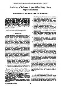
The data set is split in a left node (L) and a right node (R) in such a way that the sum of the squared differences between the observed and the average value is minimal. The stopping criterion is set as a minimum of 10 observations at the terminal nodes. Fig. 1 presents a binary regression tree constructed by applying CART to the ISBSG R11 data set. The good comprehensibility of regression trees can be considered a strong point of this technique. To determine the effort needed for a new project, it is sufficient to select the appropriate branches based on the characteristics of the new project. It is possible to construct an equivalent rule set based on the obtained regression tree (Fig. 1, bottom). This technique has previously been applied within a software effort prediction context where it consistently was considered to be one of the better performing techniques [13] [12] [27] [23].

3.3

Neural networks

Neural networks (NNs) are mathematical representations inspired by the functioning of the human brain. Many types of neural networks have been suggested in the literature [7]. In the field of software effort prediction, multilayer perceptron (MLP) networks are the most common used type of

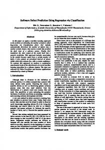
Figure 2: Neural network with one hidden layer

Figure 1: Pruned CART tree (ISBSG R11)

neural networks. A MLP is typically composed of an input layer, one or more hidden layers and an output layer, each consisting of several neurons. With the inputs of each of the neurons, a weight is associated. Assume wm is the vector of weights associated with the inputs of the mth hidden unit and vm is the scalar representing the weight associated with the output of the mth hidden unit. The output of the hidden units are calculated by a hyperbolic tangent transfer function, tanh(ξ). tanh(ξ) =

(eξ − e−ξ ) (eξ + e−ξ )

The final effort prediction, eˆ, is formed by taking the sum of the outputs of the hidden units and correcting for the output bias τ . Other transfer functions are possible. Fig. 2 illustrates the principle of a feedforward NN. eˆi =

H ∑

tanh(x′i wm )vm + τ

m=1

The network is trained by minimizing the sum of squared errors E(w, v) augmented with a complexity penalizing term P (w, v): E(w, v) =

N ∑

(ˆ ei − ei )2 + P (w, v)

minimizing the sum of the squared deviations: min

K ∑

ξ0 ,β0 ,β1

(tanh(ξi ) − L(ξi ))2 ,

i=1

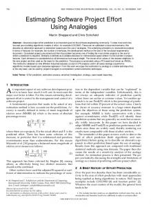
where ξi = vi′ w, the weighted input of sample i, i = 1, 2, . . . N and  if ξ < −ξ0  −α1 + β1 ξ β0 ξ if − ξ0 ≤ ξ ≤ ξ0 L(ξ) =  α +β ξ if ξ > ξ0 1 1 As tanh(0) = 0, L(0) is also fixed at 0. Due to symmetry of the tanh(ξ) function, the slope of the first and third line segment are equal and the intercept between the first (third) and the middle line segment is −ξ (ξ). A set of comprehensible IF-THEN regression rules can be extracted as the hyperbolic tangent transfer function for each hidden neuron m = 1 . . . H is approximated by a 3piece linear function. The procedure for rule extraction is as follows. • The input space is divided into 3H subregions by using the pair of intercepts (ξ and −ξ) from the function Lm (ξ). • For each non-empty subregion, a rule is generated as follows: 1. Define a linear equation that approximates the network’s output for input sample i in this subregion as the consequence of the rule:

i=1

Once the network has been trained, irrelevant and redundant hidden units and input units are removed from the network by applying the algorithm N2PFA (Neural Network Pruning for Function Approximation) [41].

3.4 Regression rule extraction A set of regression rules can be induced from the trained NN by applying REFANN (Rule Extraction from Function Approximating Neural Networks) [39] [42]. This technique uses a piece-wise linear approximation, L(ξ), of the hyperbolic tangent activation function, tanh(ξ), consisting of three line segments, Fig. 3. The 3-piece linear approximation, L(ξ), is obtained by

eˆi ξmi

= =

H ∑

vm Lm (ξmi ) + τ

m=1 x′i wm

2. Generate the rule condition: (C1 and C2 and · · · CH ), where Cm is either ξmi < −ξm0 , −ξm0 ≤ ξmi ≤ ξm0 , or ξmi > ξm0 . Thus, a rule set which is equivalent to the pruned NN with 3-piece linear approximation can be represented in the following form: ξm1 , ξm2 . . . ξmH ∈ R, the intercepts of the 3-piece linear approximation of the H hidden neurons which determine the regions.

tanh(ξ)

and 1.5

y = α1 + β1 ξ

L(ξ)

⋄⋄

0.5 0 ⋄

-0.5 -1 ⋄ ⋄

⋄

⋄ ⋄⋄ ⋄

⋄

⋄9

⋄⋄⋄ ⋄⋄ ⋄ ⋄⋄ ⋄⋄ ⋄ (−ξ0 , −β0 ξ0 )

⋄⋄ ⋄⋄ ⋄ ⋄ i

-3

-2

-1

y = β0 ξ

tanh(ξ)

sample-points

⋄

3-piece-approx. L(ξ)

y = −α1 + β1 ξ

-4

q

(ξ0 , β0 ξ0 )

1

0

1

2

3

4

ξ = weighted inputs

Figure 3: The 3-piece linear approximation of the hidden unit activation function tanh(ξ) given 30 training samples (⋄). Rule 1: IF Region 1 THEN eˆi = E1 Rule 2: IF Region 2 THEN eˆi = E2 ... Rule P: IF Region P THEN eˆi = EP with P the number of non empty regions and ∑ vm Lm (x′i wm ) + τ E1 = H ∑m=1 H E2 = m=1 vm Lm (x′i wm ) + τ ... ∑ ′ EP = H m=1 vm Lm (xi wm ) + τ with xi the input samples that lies within the associated region.

4. EMPIRICAL SET-UP In this section, background information concerning the data set used is given and the data preprocessing steps are detailed. The set-up of the study and the different evaluation criteria to assess the techniques are also discussed.

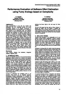
4.1 Data set The ISBSG, International Software Benchmarking Standards Group, is a not-for-profit organization that maintains a large data set of software project data 2 . This data set is often used by researchers (e.g. [20] [29] [38] [23]). In this study, ISBSG R11 (May 2009) is used containing 5052 projects collected from companies worldwide; Fig. 4 gives a breakdown of the origin of the projects. The data relates to projects collected from 1992 up until 2009. For this study, 721 projects were selected according to the following criteria. • Only projects with an overall data quality of A or B and a function point quality of A were selected. • The function points needed to be counted by the IFPUG 4 standard 3 . 2

www.isbsg.org 3 www.ifpug.org/publications/manual.htm

Figure 4: Breakdown of the origin of the projects • Projects with missing values for team size, function point count or effort were discarded. • The total effort recorded must be related only to development effort. Table 2 provides an overview of the parameters included in the data set. In case of categorical variables with more than 8 possible values, some of the levels were merged to obtain a more concise data set. This merging was based on semantic similarity. Levels with less than 15 observations, were put in a category named ‘Other’ in line with a study done by Jeffrey et al. [23]. The categorical variables were transformed into binary variables by applying dummy encoding as the categorical attributes are nominal by nature [5]. A missing data flag was created to account for missing values. No outlier removal or other preprocessing steps were applied.

4.2 Study set-up To obtain a fair estimation of performance of the various techniques, the data is randomly split into a training and a test set containing 649 projects and 72 projects respectively.

Table 2: Overview of the attributes used Variable name Effort TeamSize FunctionCount ApplType Arch Database DevPlat DevType LanType Lan OrgType Meth

Variable description total effort of the project in man hours number of developers working on the project size of the project, expressed in function points application type (e.g. financial appl.) architecture (e.g. client-server) primary database used in the project development platform (e.g. mainframe) development type (e.g. new dev.) language generation language used for the project organization type methodology used during development

Type cont. cont. cont. cat. cat. cat. cat. cat. cat. cat. cat. cat.

The techniques are trained using only data contained in the training set and afterwards evaluated using the previously unseen data from the test set. A key question of any estimation method is whether the predictions are accurate; the difference between the actual effort, ei , and the predicted effort, eˆi , should be as small as possible. The two most common used criteria in the context of software effort prediction are MMRE and Pred(25). Both are derived from the Magnitude of Relative Error (MRE) [14]. The MRE is calculated for each observation and is defined as: |ei − eˆi | M REi = ei The MMRE (Mean MRE) is defined as: M M RE =

N 100 ∑ |ei − eˆi | N i=1 ei

A complementary accuracy measure is Pred(L) [14], the fraction of observations for which the predicted effort, ei falls within L% of the actual effort, eˆi : N { L 100 ∑ 1 if M REi ≤ 100 P red(L) = 0 otherwise N i=1 Typically, the Pred(25) measure is considered, looking at the percentage of predictions that are within 25% of the actuals. While both measures are based on the MRE, they have a slightly different focus; Pred(L) is favoring models which are generally accurate but occasionally widely inaccurate. MMRE on the other hand can be highly affected by outliers [35]. To address this shortcoming in the MMRE measure, the MdMRE is also considered. The MdMRE is the median of all MREs and thus can be considered more robust against outliers. M dM RE = 100 ∗ median(M RE) Finally, the techniques are also assessed using the R2 measure. This measure reflects the percentage of variation that is being explained by the model: ∑N (ei − eˆi )2 SSerr 2 = 1 − ∑i=1 R =1− N 2 SStot i=1 (ei − e) R2 is a value between 0 and 1 with 1 meaning all the variation in the data is explained by the model. The results obtained on the independent test set are tested using one way ANOVA (ANalysis Of VAriance). This statistical technique assesses the question whether the mean across multiple groups are different by taking the variances

of the groups into account, hence its name. The results are tested at statistical significance level α = 0.01. Following the ANOVA test, Tukey’s honest significance test is utilized to perform a pairwise comparison of the techniques in order to investigate whether the differences between two specific techniques are statistically significant. A statistical significance level of α = 0.05 is used for this second test.

5.

RESULTS

In a first part of the experiment, the three techniques (OLS, CART and rule extraction from NNs) are compared to each other in terms of MMRE, MdMRE, Pred(25) and R2 . The results of the experiments are displayed in Table 3. It can be seen that CART provides the best overall results while the rule extraction algorithm is second except when the R2 is considered. However, analysis of the CART tree shows that the resulting tree consists of 47 splitting nodes. The induced rule set thus consists of 48 rules with in some cases up to 10 rule antecedents. The CART tree can thus be considered too elaborate to be easily comprehensible by the business. The rule set induced from the pruned NN is considerably smaller, only containing 5 rules with at most 2 rule antecedents. The rule set obtained from the pruned NN is given in Table 4. In a second part of the experiment, we further pruned the CART tree in order to obtain the same complexity of rule set (the same number of rules and rule antecedents) as the rule set extracted from the pruned NN. The results are indicated in Table 3 as ‘CART pruned’ and the CART tree as well as the induced rule set are shown in Fig. 1. It can be concluded from the results that the NN rules perform better than the pruned CART tree in terms of MMRE, MdMRE, Pred(25) and R2 . Fig. 5 shows box plots for the 4 techniques of the MMRE. The median value which is displayed in the box plots is the MdMRE which is also provided in Table 3. To further assess the statistical significance of the results, an ANOVA is performed to test whether the MMRE is significantly different across the 4 techniques (OLS, CART, CART pruned and Rule extraction from NN). The null hypothesis is the following: H0 : MMRECART = MMREOLS = MMRECARTpruned = MMRERules The results of the ANOVA are given in Table 5. The test is significant at 1 % (p=0.000149) thus it can be concluded that the MMRE across the 4 techniques is statistically different. Following the ANOVA, a Tukey’s honest significance test is performed which does a pairwise comparison of the different techniques. The null hypothesis is given below. H0 : MMREk = MMREl with k ̸= l The results of this test are displayed in Table 6. In boldface font the significant pairwise differences are given (criti-

Table 3: Results OLS Cart Cart Pruned NN + rule extraction

Pred(25) 22.22 37.50 16.67 30.56

MMRE 135.03 61.16 186.45 95.39

MdMRE 57.06 39.87 77.05 57.25

R2 -0.8914 0.835 0.806 0.882

cal value = 3.722). It can concluded from these tests that the regression rules extracted from the NN are significantly better performing than the pruned CART tree (MMRECARTpruned = 186.45 versus MMRERules = 95.39). The CART tree without additional pruning is the best performing technique at the expense of a larger and thus less comprehensible rule set although this result is only statistically significant when compared to the pruned CART tree. When CART is compared with OLS, the result is very close to the critical value (3.625 as compared to the critical value = 3.722). Table 4: Rule set extracted from NN Equivalent rule set Rule 1 IF Region 1 AND DevType = Enhan THEN 496.98 + 1.74 × FunctionCount + 428.32 × TeamSize Rule 2 IF Region 1 AND DevType ̸= Enhan THEN -776.42 + 1.74 × FunctionCount + 428.32 × TeamSize Rule 3 IF Region 2 THEN -15705.45 + 10.59 × FunctionCount + 778.27 × TeamSize Rule 4 IF Region 3 THEN 5859.29 + 9.02 × FunctionCount + 365.39 × TeamSize Rule 5 IF Region 4 THEN 55637.90 + 0.16 × FunctionCount + 15.50 × TeamSize Intercepts of the hidden neurons, ξmi ξm1 = 92.63 ξm2 = 140.18 Region demarcation Region 1 x′i wm ≤ ξm1 AND x′i wm ≤ −ξm2 Region 2 x′i wm ≤ ξm1 AND x′i wm ≤ ξm2 Region 3 x′i wm ≥ ξm1 AND x′i wm ≤ ξm2 Region 4 x′i wm ≥ ξm1 AND x′i wm ≥ −ξm2

Table 5: ANOVA results Source of Variation DF Type III SS Between Groups 3 627079.73 Within Groups 284 8492851.59 F value F valuecritical p value 6.9898 3.8513 0.000149

Table 6: Tukey’s honest significance test CART

CART OLS CART Pruned NN + rule extraction

OLS

3.625 3.626 6.148 1.680

2.523 1.945

CART Pruned

6.148 2.523

NN + rule extraction 1.680 1.945 4.468

4.468

6. CONCLUSIONS This experimental study assessed the feasibility of regression rule extraction from Neural Networks (NNs) in the context of software effort prediction. The algorithm generates a small number of linear equations from a neural network trained for regression. The analysis on the ISBSG R11 data set indicated that the performance of the rule set obtained by applying the REFANN (Rule Extraction from Function 4

The negative R2 is due to an outlier in the test set; removing this outlier, we obtained an R2 = 0.34

Figure 5: Box plot of MMRE for the different techniques Approximating Neural Networks) algorithm on a trained and pruned NN is on par with other techniques. However, the regression rule extraction algorithm provides the end user with a more concise set of rules (both in terms of the number of rules and the number of rule antecedents) than the CART (Classification And Regression Tree) algorithm which is commonly used in the literature. Therefore the idea of regression rule extraction should be considered of high relevance to the practical implementation of software effort prediction systems in a business environment where comprehensibility is of high importance. Further research on the usability of the algorithm on other software effort prediction data sets is needed to assess this technique more in depth. Other types of rule extraction algorithms are currently investigated by the authors.

7.

ACKNOWLEDGMENTS

This research was supported by the Odysseus program (Flemish Government, FWO) under grant G.0915.09. We would also like to thank the Flemish Research Fund for financial support to the authors (Odysseus grant G.0915.09 to Bart Baesens and post-doctoral research grant to David Martens).

References [1] A. Abran and P. N. Robillard. Function points analysis: An empirical study of its measurement processes. IEEE Transactions on Software Engineering, 22(12):895–910, 1996. [2] A. J. Albrecht and J. E. Gaffney. Software function, source lines of code, and development effort prediction: A software science validation. IEEE Transactions on Software Engineering, 9(6):639–648, 1983. [3] B. Baesens, T. V. Gestel, S. Viaene, M. Stepanova, J. Suykens, and J. Vanthienen. Benchmarking state-ofthe-art classification algorithms for credit scoring. Journal of the operational research society, 54(6):627–635, 2003. [4] B. Baesens and C. Mues. Recursive neural network rule extraction for data with mixed attributes. IEEE Transactions on Neural Networks, 19(2):299–307, 2008.

[5] B. Baesens, R. Setiono, C. Mues, and J. Vanthienen. Using neural network rule extraction and decision tables for credit-risk evaluation. Management Science, 49(3):312–329, 2003.

[20] S.-J. Huang and N.-H. Chiu. Optimization of analogy weights by genetic algorithm for software effort estimation. Information and Software Technology, 48(11):1034–1045, 2006.

[6] J. W. Bailey and V. R. Basili. A meta-model for software development resource expenditures. In Proc. of the fift International Conference on Software Engineering, 107–116, 1981.

[21] A. Idri, T. M. Khoshgoftaar, and A. Abran. Can Neural Networks be easily Interpreted in Software Cost Estimation ? In Proc. of the IEEE International Conference on Fuzzy Systems, pages 1162–1167, Honolulu, Hawaii, 2002.

[7] C. M. Bishop. Neural networks for pattern recognition. Oxford University Press, 1995. [8] J. Bode. Neural networks for cost estimation: simulations and pilot application. International Journal of Production Research, 38(6):1231–1254, 2000. [9] B. Boehm. Software Engineering Economics. Prentice Hall, New Jersey, 1981. [10] B. Boehm, C. Abts, and S. Chulani. Software development cost estimation approaches - A survey. Annals of Software Engineering, 10(4):177–205, 2000. [11] L. Breiman, J. H. Friedman, R. A. Olsen, and C. J. Stone. Classification and Regression Trees. Wadsworth & Books/Cole Advanced Books & Software, 1984. [12] L. Briand, K. E. Emam, D. Surmann, and I. Wieczorek. An assessment and comparison of common software cost estimation modeling techniques. In Proc. of the 21st international conference on Software engineering, pages 313–323, Los Angeles, California, May 1999. [13] L. Briand, T. Langley, and I. Wieczorek. A replicated assessment and comparison of common software cost modeling techniques. In Proc. of the 22nd international conference on Software engineering, pages 377– 386, Limerick, Ireland, June 2000. [14] S. D. Conte, H. E. Dunsmore, and V. Y. Shen. Software engineering metrics and models. The Benjamin/Cummings Publishing Company, Inc, Redwood City, CA, USA, 1986. [15] J. M. Desharnais. Analyse statistique de la productivities des projets de developpement en informatique apartir de la techniques des points de fonction. PhD thesis, University du Quebec, Quebec, Canada, 1988. [16] J. J. Dolado. A study of the relationships among albrecht and mark II function points, lines of code 4GL and effort. Journal of Systems and Software, 37(2):161– 173, 1997. [17] G. Finnie, G. Wittig, and J.-M. Desharnais. A comparison of software effort estimation techniques: Using function points with neural networks, case-based reasoning and regression models. Journal of Systems and Software, 39:281–289, 1997. [18] A. Heiat. Comparison of artificial neural networks and regression models for estimating software development effort. Information and Software Technology, 44(15):911–922, 2002. [19] K. Hornik, M. Stinchcombe, and H. White. Multilayer feedforward networks are universal approximators. Neural Networks, 2(5):359–366, 1989.

[22] A. Idri, A. Zahi, E. Mendez, and A. Zakrani. Software Cost Estimation Models Using Radial Basis Function Neural Networks. In Lecture Notes in Computer Science, volume 4895, pages 21–31, 2008. [23] R. Jeffery, M. Ruhe, and I. Wieczorek. Using public domain metrics to estimate software development effort. In Proc. of the Seventh International Software Metrics Symposium, pages 16–27, London, UK, April 2001. [24] M. Jørgensen and M. Shepperd. A systematic review of software development cost estimation studies. IEEE Transactions on Software Engineering, 33(1):33– 53, 2007. [25] G. Kateman and J. R. M. Smits. Colored information from a black box ? Validation and evaluation of neural networks. Analytica Chimica Acta, 277(2):179–188, 1993. [26] C. F. Kemerer. An empirical validation of software cost estimation models. Communications of the ACM, 30(5):416–429, 1987. [27] B. Kitchenham. A procedure for analyzing unbalanced data sets. IEEE Transactions on Software Engineering, 24(4):278–301, 1998. [28] H. K. Leung. Estimating maintenance effort by analogy. Empirical Software Engineering, 7:157–175, 2002. [29] J. Li, G. Ruhe, A. Ak-Emran, and M. Richter. A flexible method for software effort estimation by analogy. Empirical Software Engineering, 12:65–107, 2007. [30] D. Martens, B. Baesens, T. Van Gestel, and J. Vanthienen. Comprehensible credit scoring models using rule extraction from support vector machines. European journal of operational research, 183(3):1466–1476, 2007. [31] E. Mendes, S. Counsell, and N. Mosley. Measurement and effort prediction for web applications. Lecture notes in computer science, 2016:295–310, 2000. [32] E. Mendes, N. Mosley, and S. Counsell. Web metrics - estimating design and authoring effort. IEEE Multimedia, Special Issue on WebEngineering, 8(1):50–57, 2001. [33] E. A. Nelson. Management Handbook for the Estimation of Computer Programming Costs. System Developer Corp., 1966. [34] M. Pazzani, S. Mani, and W. Shankle. Acceptance by medical experts of rules generated by machine learning. Methods of Information in Medicine, 40(5):380– 385, 2001.

[35] D. Port and M. Korte. Comparative Studies of the Model Evaluation Criterions MMRE and PRED in Software Cost Estimation Research. In Proc. of the Second ACM-IEEE international symposium on Empirical software engineering and measurement, pages 51– 60, Kaiserslautern, Germany, October 2008. [36] L. H. Putnam. A general empirical solution to the macro software sizing and estimation problem. IEEE Transaction on Software Engineering, 4(4):345–381, 1978. [37] J. R. Quinlan. C4.5: programs for machine learning. Morgan Kaufmann, 2003. [38] P. Sentas, L. Angelis, I. Stamelos, and G. Bleris. Software productivity and effort prediction with ordinal regression. Information and Software Technology, 47:17– 29, 2005. [39] R. Setiono. Generating linear regression rules from neural networks using local least squares approximation. In Proc. of the 6th International Work-Conference on Artificial and Natural Neural Networks, volume 1, pages 277–284, Granada, Spain, 2001. [40] R. Setiono, B. Baesens, and C. Mues. Recursive neural network rule extraction for data with mixed attributes. IEEE Transactions on Neural Networks, 19(2):299–307, 2008. [41] R. Setiono and W. K. Leow. Pruned neural networks for regression. In Proc. of the 6th Pacific Rim Conference on Artificial Intelligence, Lecture notes in AI, volume 1886, pages 500–509, San Mateo, CA, 2000. [42] R. Setiono, W. K. Leow, and J. M. Zurada. Extraction of rules from artificial neural networks for nonlinear regression. IEEE Transactions on Neural Networks, 13(3):564–577, 2002. [43] R. Shukla and A. Misra. Estimating software maintenance effort- a neural network approach. In Proc. of the 1st conference on India software engineering conference, pages 107–112, Hyderabad, India, February 2008. [44] K. Srinivasan and D. Fisher. Machine learning approaches to estimating software development effort. IEEE Transactions on Software Engineering, 21(2):126–137, 1995. [45] P.-N. Tan, M. Steinbach, and V. Kumar. Introduction to Data Mining. Addison Wesley, Boston, MA, 2005. [46] The Standish Group. Chaos report. Technical report, http://www.standishgroup.com, 2009. [47] L. Torgo and J. Gama. Search-based class discretization. In Proc. of the 9th European Conference on Machine Learning, Lecture Notes in AI, volume 1224, pages 266–273, Prague, Czech Republic, 1997. Springer. [48] D. Treigueiros and R. Berry. The application of neural network based methods to the extraction of knowledge from accounting reports. In Proceedings of 24th Annual Hawaii International Conference on Systems Sciences, volume 4, pages 137–146, Hawaii, 1991.

[49] O. Vandecruys, D. Martens, B. Beasens, C. Mues, M. De Backer, and R. Haesen. Mining software repositories for comprehensible software fault prediction models. The Journal of Systems and Software, 81(5):823, 2008. [50] C. E. Walston and C. P. Felix. A method of programming measurement and estimation. IBM Systems Journal, 16(1):54–73, 1977. [51] B. Widrow, D. E. Rumelhart, and M. A. Lehr. Neural networks: applications in industry, business and science. Communications of the ACM, 37(3):93–105, 1994. [52] G. Wittig and G. Finnie. Estimating software development effort with connectionist models. Information and Software Technology, 39(7):469–476, 1997.