Solar Power Prediction via Support Vector Machine and Random Forest

E3S Web of Conferences 69, 01004 (2018) Green Energy and Smart Grids 2018

https://doi.org/10.1051/e3sconf/20186901004

Solar Power Prediction via Support Vector Machine and Random Forest Chih-Feng Yen1, He-Yen Hsieh1, Kuan-Wu Su1, Min-Chieh Yu1 and Jenq-Shiou Leu1 1 Department of Electronic and Computer Engineering, National Taiwan University of Science and Technology, Taiwan Abstract. Due to the variability and instability of photovoltaic (PV) output, the accurate prediction of PV output power plays a major role in energy market for PV operators to optimize their profits in energy market. In order to predict PV output, environmental parameters such as temperature, humidity, rainfall and win speed are gathered as indicators and different machine learning models are built for each solar panel inverters. In this paper, we propose two different kinds of solar prediction schemes for one-hour ahead forecasting of solar output using Support Vector Machine (SVM) and Random Forest (RF)

1 Introduction In recent years, the global warning and extreme weather conditions have become more and more severe due to the massive production of greenhouse gases. A variety of renewable energy sources play more important roles in energy production markets globally, and alternative power grids gradually replace traditional fossil fuel based power plants. Within these renewable energy sources, solar power plays an important role, not only does it generates clean energy with no pollution, but also as an important constituent in a realistic smart grid system for distributed photovoltaic (PV) operators [1]. Solar power system production is expected to rapidly increase until 2030 due to its low building and maintenance cost [2]. In past studies, the characteristics of solar energy data show periodicity depended upon weather conditions such as cloud, humidity, precipitation, wind speed, temperature and dew point [3]. Due to its nature of fluctuating energy output across different hours, PV systems may cause imbalance in power dispatching within the connected energy grid. Thus, PV operators have disadvantage in the power trading market, which imposes penalties due to prediction errors [4]. However, the internal data still show instability sometimes. Thus better prediction methods for PV systems’ solar inverters are increasingly become the most important tasks for PV operators. There have been a number of studies on the prediction of solar irradiance and PV output power where its output was gathered as time-series data using methods such as Autoregressive Moving Average (ARMA)[5], ARMA can be used to obtain the prediction models by characteristics of solar irradiance [6][7]. Although it can predict the electricity generation rapidly, it shows low accuracy due to non-stationary characteristics of the

solar irradiance time series, since the prediction accuracy depends on various meteorological factors such as cloud cover, humidity, temperature and wind speed instead of purely past temporal correlations and patterns [8]. To overcome these shortcomings, nonlinear prediction schemes based on machine learning can be used to predict electricity generations more accurately. For instance, schemes like SVM [9], and RF [10][11]. Weather-based SVM methods have been used in forecasting PV output power. They have made significant progress in predicting solar output and have greatly improved their accuracy over the years [9]. RF also has been used in prediction using ensemble learning models [10], where multiple models can be integrated to further improved the predicting capability over time [11]. In this paper we utilize two different machine learning methods Support Vector Machine (SVM) and Random Forest (RF) to predict individual PV inventor output and compare their performances, where Section II illustrates related works and backgrounds for these two machine models, and Section III describes the architecture and evaluation metrics. Section IV provides experiment results with conclusions and future works listed in Section V.

2 Related Works 2.1 Support Vector Machine Support Vector Machine (SVM) is widely used due to the versatile performance of solving non-linear problems, even when trained with small datasets. It can be used both for classification and regression tasks where the regression version being called Support Vector Regression (SVR).

*

Corresponding author: [email protected]

© The Authors, published by EDP Sciences. This is an open access article distributed under the terms of the Creative Commons Attribution License 4.0 (http://creativecommons.org/licenses/by/4.0/).

E3S Web of Conferences 69, 01004 (2018) Green Energy and Smart Grids 2018

https://doi.org/10.1051/e3sconf/20186901004

For a given observation sample set of N input and output data D = {(𝑥𝑥1 , 𝑦𝑦1 ), (𝑥𝑥2 , 𝑦𝑦2 ), … , (𝑥𝑥𝑁𝑁 , 𝑦𝑦𝑁𝑁 )} ∈ 𝑅𝑅𝐾𝐾 × 𝑅𝑅. Its regression function is expressed as F{f|f(xi = W T ∙ xi + b, w ∈ RK )}

(1)

where w is the unit normal vector to the hyperplane, b is the distance from the origin to the hyperplane, and 𝑥𝑥𝑖𝑖 is the input vector. The key idea of the non-linear SVM is to map the input vectors into high-dimensional feature space by using a nonlinear mapping process. In such a higherorder space, there is a higher possibility that the data can be linearly separated [1]. The problem can be formulated as: 1

min( ‖𝑤𝑤‖2 + C ∑𝑀𝑀 𝑖𝑖=1 ζi) 2

subjects to boundary conditions

𝑦𝑦𝑖𝑖 (𝑊𝑊 𝑇𝑇 ∙ 𝜑𝜑(𝑥𝑥𝑖𝑖 ) + 𝑏𝑏) ≥ 1 − ζi, ζi ≥ 0

(2) (3)

where ζi is a slack variable, M is the number of input and output data for training, and C is the cost function regularization parameter. The cost function C determine the accuracy of the model. When C value is large, it makes the model more accurately but it may occur the overfitting. On the other hand, when C value is small, it will look for a large-spaced hyperplane. In this case, if your training set is linearly separable, there may be misclassified samples. The mapping function 𝜑𝜑(𝑥𝑥𝑖𝑖 ) in the high-dimensional space can be replaced by special kernel functions K �𝑥𝑥𝑖𝑖 , 𝑥𝑥𝑗𝑗 � , and all the necessary computations can be performed directly in the input space by calculation kernels using kernel methods.

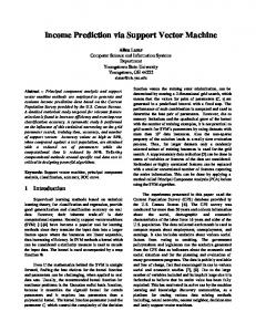
Figure 1. The flowchart of Random Forest

3 Architecture and evaluation methods Fig. 2. shows the flowchart of our proposed models. It contains two machine learning modules, Support Vector Regression (SVR) and Random Forest (RF) to predict the PV solar electricity generation. The scheme to generate prediction machine learning models has three stages. First, data gathered from solar invertors of local PV operators and using crawlers to automatically collect weather condition information from weather observation stations of Taiwan Central Weather Bureau[12]. And then the collected data is aggregated and preprocessed for detecting outlier values and imputing missing items to produce complete time series training data, hence machine learning models can train these preprocessed data easily and effectively. After the processed data being trained by SVR and RF-regression modules, the generated perdition models for individual PV solar panel can now be used to predict future electricity generation output. Finally, we compare the predictions using testing data with four evaluation metrics: Mean Absolute Error (MAE), Root Mean Square Error (RMSE), Mean Forecast Error MFE) and Mean Absolute Scaled Error (MASE).

2.2 Random Forest Random forest is a combinatorial classifier and can be used for regression as well. The main idea of RF is constructing several decision trees at training time and ensembles the results generated from individual trees. RF is based on a decision tree using a random selection of attributes for each node of the decision tree. First, from the attributes of the nodes in the random selection of servers attribute subsets, and then from the subset to select an optimal attribute for node splitting, which can make each decision tree different, enhance the diversity of the system. And then construct multiple decision trees and order of variables randomly. Finally, it gets the classification results by voting method, so as to enhance the classification performance, flow chart of the RF is shown in Figure 1. Following the steps, RF often gets better accuracy than each decision tree and can deal with large datasets. The major parameters for random forest method are tree depth and number of trees which are not sensitive, and can be easily applied to PV solar power output prediction here.

2

E3S Web of Conferences 69, 01004 (2018) Green Energy and Smart Grids 2018

https://doi.org/10.1051/e3sconf/20186901004

Also the possible solar production output value limit is applied based on the internal circuit sensor measurements. However, the uncertainty of circuit failure and solar production degradation due to the aging of equipment’s can also cause unreliable readings. Right now we accept there are errors introduced in the observed data, where more advanced detection methods to determine the integrity of the system and gathered data can be included to further improve the reliability of source data. For imputing missing time-series data points, there are several different methods can be applied. From simply asserting fixed value, replacing them according to statistical guidelines and rules, to interpolation methods, to imputation methods and complex estimation methods. In this study, several different imputation techniques are applied in order to facilitate the restoration of a complete dataset that can be used in machine learning modules. In the weather condition historical data, there are many missing segments consist of just one single missing data point, however the rest of the missing segments usually ranged in days of dozens of missing data points. Hence in order to fill the missing data segments we applied the technique of Inverse Distance Weighting method[14] where the meteorological data from observation stations around the target observation stations with missing values are used. The inverse values of the distances to the target station are used as weights to interpolate these missing time period data. The equation for Inverse Distance Weighting method is shown in equation (4).

Figure 2. The flowchart of the proposed model

3.1 Data gathering In order to build a solar production model realistically, we gathered PV solar power output data directly from manufacturers of PV solar systems. The data gathered by solar investors which have been installed and integrated in to current smart power grid over the years are stored into an online database[13], and these raw data from the PV system circuits can be exported for further analysis. For gathering weather condition information within the local area of the target PV solar system, we survey the online weather observation data inquire system database from Taiwan Central Weather Bureau[12] to locate the nearest observation station within mesoscale weather region. After that we use web crawlers to gather historic data within the same solar power production dataset time period, and stored them in the local database.

z𝑗𝑗 ′ =

1 ) d𝑖𝑖𝑖𝑖 1 𝑀𝑀 ∑𝑖𝑖=1( 𝑟𝑟 ) d𝑖𝑖𝑖𝑖

∑𝑀𝑀 𝑖𝑖=1 𝑧𝑧𝑖𝑖 (

(4)

where z𝑗𝑗 ′ is the interpolated target station j weather condition value, and z𝑖𝑖 are weather condition values from neighboring M weather stations with their distance to station j as d𝑖𝑖𝑖𝑖 and the inverse coefficient parameter r, usually sets to 2. On the other hand, some weather condition value is usually limited and bind within local area, such as rain fall, the method of interpolation is more suited using Nearest Neighbor method where the missing data point is filled with the mean value from its geographically nearest neighbors within certain range. Another accompany approach is to find weighted mean value through historical record of the same time of similar patterns but different years if nearest geological neighbors’ values cannot be obtained, or all of them lack valid values in the missing data period. The gathered solar invertor output data also contains missing data points from either equipment malfunctions or from the earlier data cleaning process. On top of that, during night times, PV solar systems are turned off thus only data points during sunlight hours are presented in the database. Along with the fact that we don’t have enough close by PV solar output to be used for interpolating value through spatial correlation, hence in order to construct valid training dataset where the training target solar invertor output level are highly fragmented in time, we applied a technique called Local

3.2 Preprocessing Time-series data gathered through different channels mentioned above usually contains some missing data points and outliers of anomaly readings, hence in order to build machine learning models of higher accuracy we required data preprocessing step of data cleaning to find and eliminate outlier data points, as well as to impute missing data points. In order to find outlier values in weather condition data, we survey possible regional weather condition values as well as weather database combined with the knowledge of weather observation through meteorology.

3

E3S Web of Conferences 69, 01004 (2018) Green Energy and Smart Grids 2018

https://doi.org/10.1051/e3sconf/20186901004

Mean Absolute Scaled Error (MASE) is a modern measurement proposed more recently developed in order to alleviate certain problems existed in traditional forecast accuracy measurements, such as scale dependency hence difficult to compare between different dataset at different scale, or asymmetry in data absolute scale and distinguish underestimated and overestimated the trend within the scope of time-series data. The equation for MASE is shown in equation (8).

Time Index (LTI)[15], where the dataset are treated as segments of discrete events in time with time index as variables joint together to form event records, replacing a fixed interval continue stream of time series data. By matching these target time label with weather condition data, time depended training dataset with event records can be generated for the machine learning modules to train. 3.3 Evaluation Metrics

𝑀𝑀𝑀𝑀𝑀𝑀𝑀𝑀 =

In this study, we used four evaluation metrics to measure the forecasting performance. Each of them has advantages and disadvantages. Based on these metrics, we can analyze the trends of the results. These metrics are Mean Absolute Error (MAE), Root Mean Square Error (RMSE), Mean Forecast Error (MFE) and Mean Absolute Scaled Error (MASE) respectively. If we define time-series data from time period of 𝑡𝑡 = 1~𝑛𝑛 with the observed actual value of the time sequence noted as 𝑦𝑦𝑡𝑡 and predicted forecast time sequence as 𝑦𝑦𝑡𝑡 ′ , then these four measurements are defined as follows:

4.1 Experiments setup In this experiment, the gathered weather condition data is from an observation station in southern Taiwan located in the same town as the targeted PV solar output system for forecasting. The distance between the observation station and the PV solar operator’s location is 1.28 km. And the available weather condition data is collected from 2017/1/1 00:00 hour to 2018/4/30 23:00 hour of the same county where the town resides. The available PV solar invertor data is collected between 2015/1/1 06:00 hour to 2018/4/30 18:00 hour from 22 different PV solar invertors. Considering the overlapping time frames between weather conditions and PV output data, we select the whole year of 2017 from 2017/1/1 00:00 hour till 2017/12/31 23:00 hour as the time-series training data, with the testing data from 2018/1/1 00:00 hour till 2018/4/30 18:00. For machine learning modules, the parameters of margins ε and the cost function regularization parameter C for SVM are set to 0.1 and 1 respectively. And the kernel function of SVM uses Radial Basis Function (RBF) which is easier to map the nonlinear data to high dimensional space. The parameters of the number of trees in the forest and the tree depth of RF are set from 50 to 100 and pick the best performance as results.

Mean Absolute Error (MAE) measures the difference between two continuous time series with their average magnitude of errors without considering their directions. It tells the average and absolute differences between prediction and actual observation values where all individual differences have the same weight. The equation of calculating MAE is shown in equation (5). 1

𝑛𝑛

3.3.2 Root mean absolute error:

(5)

Root Mean Square Error (RMSE) is a commonly used measurement of the differences between observed and predicted values. It represents the sample standard deviation of the differences. It’s the square root of the Mean Square Error (MSE). Large errors have larger effect compared to small errors, hence it is sensitive to outliers if the data is not properly preprocessed. The equation of calculating RMSE is shown in equation (6). 𝑅𝑅𝑅𝑅𝑅𝑅𝑅𝑅 =

1

� ∑𝑛𝑛𝑡𝑡=1(𝑦𝑦𝑡𝑡 𝑛𝑛

3.3.3 Mean forecast error:

− 𝑦𝑦𝑡𝑡 ′)2

4.2 Experiments results The evaluation metrics of testing results from 22 PV solar output between observed and prediction values are listed in Table 1, with best prediction result highlighted in bold text and lighter individual cell background color for better forecasting value compared to observed data. Across the forecasting results, RF performs better than SVM prediction results, where RF slightly overestimate actual output values, and SVM underestimate them. In terms of other measurements RF performs about 37% to 40% better in terms of RMSE, MAE and MASE. Examples of forecasting output compared between observed and predicted values with and Support Vector Machine, Random Forest methods shown for a week from 2018/2/12 till 2018/2/18 are shown in Fig. 3 and Fig. 4.

(6)

Mean Forecast Error (MFE) is used as a measurement for how closely a forecast follows the trend of the data and is also called bias measurement, with positive and negative value to show on average if the prediction underestimates or overestimates the actual observed data trend. The equation for MFE is shown in equation (7). 1

𝑀𝑀𝑀𝑀𝑀𝑀 = ∑𝑛𝑛𝑡𝑡=1(𝑦𝑦𝑡𝑡 − 𝑦𝑦𝑡𝑡 ′) 𝑛𝑛

3.3.4 Mean absolute scaled error:

(8)

4 Experiments and results

3.3.1 Mean absolute error:

𝑀𝑀𝑀𝑀𝑀𝑀 = ∑𝑛𝑛𝑡𝑡=1|𝑦𝑦𝑡𝑡 − 𝑦𝑦𝑡𝑡 ′|

∑𝑛𝑛 𝑡𝑡=1(𝑦𝑦𝑡𝑡 −𝑦𝑦𝑡𝑡 ′) 𝑛𝑛 ∑𝑛𝑛 |𝑦𝑦 −𝑦𝑦𝑡𝑡−1 | 𝑛𝑛+1 𝑡𝑡=2 𝑡𝑡

(7)

4

E3S Web of Conferences 69, 01004 (2018) Green Energy and Smart Grids 2018

https://doi.org/10.1051/e3sconf/20186901004

As described above, the RF forecasting model more closely follows the actual data trend, but less so for the

SVM model. However, they both capture the pattern of daily solar production output cycle.

TABLE 1. EVALUATION METRICS OF 22 PV SOLAR INVERTOR OUTPUT PREDICTION

Data PV id01 PV id02 PV id03 PV id04 PV id05 PV id06 PV id07 PV id08 PV id09 PV id10 PV id11 PV id12 PV id13 PV id14 PV id15 PV id16 PV id17 PV id18 PV id19 PV id20 PV id21 PV id22 Average

MAE 1.7874 1.7451 1.6985 1.7938 1.7357 1.7227 1.7114 1.6515 1.7283 1.7041 1.4773 1.6805 1.7373 1.7773 1.6853 1.6625 1.6700 1.7075 1.6430 1.6316 1.6384 1.5355 1.6875

SVM

MASE 1.5302 1.4918 1.4534 1.5306 1.4882 1.4782 1.4567 1.4295 1.5021 1.4835 1.3967 1.4299 1.4998 1.5908 1.4659 1.4630 1.4714 1.4558 1.4408 1.4296 1.4217 1.4268 1.4698

MFE 1.2087 1.1340 1.1494 1.2339 1.1492 1.1248 1.1381 1.0598 1.1627 1.2014 0.9290 1.2167 1.1962 1.2898 1.1113 1.0218 1.0494 1.1581 1.0026 1.0632 1.0493 0.9211 1.1168

RMSE 2.6645 2.5758 2.4932 2.6566 2.5886 2.5771 2.5444 2.4455 2.5766 2.5724 2.1945 2.5230 2.5881 2.6109 2.5074 2.4610 2.4668 2.5664 2.4566 2.4127 2.4605 2.2647 2.5094

MAE 0.9764 0.9954 0.9941 1.0152 1.0053 0.9934 1.0000 0.9993 0.9974 0.9993 0.8889 1.0527 1.0237 1.0618 1.0388 1.0356 1.0211 1.0356 0.9875 1.0368 1.0861 0.9658 1.0096

MASE 0.8359 0.8510 0.8507 0.8662 0.8619 0.8524 0.8512 0.8650 0.8668 0.8700 0.8404 0.8957 0.8837 0.9503 0.9036 0.9113 0.8997 0.8829 0.8660 0.9085 0.9424 0.8974 0.8797

RF

MFE -0.0066 -0.0427 -0.0632 -0.0270 -0.0375 -0.0158 -0.0164 -0.0657 -0.0722 -0.0072 0.0421 0.0053 -0.0046 0.0066 -0.0276 -0.0191 -0.1028 -0.0224 -0.0408 -0.0118 0.0447 -0.0303 -0.0234

RMSE 1.5271 1.5636 1.5283 1.5791 1.5708 1.5401 1.5523 1.5794 1.5890 1.5842 1.3912 1.7037 1.6451 1.6699 1.6203 1.6430 1.5876 1.6594 1.5647 1.6271 1.6993 1.5070 1.5878

Fig. 4. Forecasting solar output (kWh) of PV invertor id01 using Random Forest Model

6 Conclusions Intelligent power grids become increasing important and they rely on renewable energy sources more and more each year. Options like PV solar power production require more researches in order to have better and more optimized energy production. Forecasting possible solar output level purely from environmental factors such as weather conditions are viable options if we can using machine learning to build prediction modules for individual solar invertors. Such mechanism can also be applied for other applications and prediction tasks such as detecting possible failures. They can also become valuable tools for PV operators to plan ahead of time for more robust financial options in the energy trading market In the future, with more embedded sensors and richer context data like current and voltage, and applying more machine learning methods, we wish to achieve even better prediction accuracy as well as longer forecasting period. Starting from gathering more data continuously and build more accurate long term pattern across several

Fig 3. Forecasting solar output (kWh) of PV invertor id01 using Support Vector Machine Model

5

E3S Web of Conferences 69, 01004 (2018) Green Energy and Smart Grids 2018

https://doi.org/10.1051/e3sconf/20186901004

years. These steps not only can provide better results over time, but also possibly be used to build real time online interactive forecasting and predicting system where machine learning modules can constantly gather data and update their forecasting capability through reinforcement learning.

12.

References 13. 1.

W. Gu, Z. Wu, R. Bo, W. Liu, G. Zhou, W. Chen, and Z. Wu, ”Modeling, Planning and Optimal Energy Management of Combined Cooling, Heating and Power Microgrid: A Review,” International Journal of Electrical Power and Energy Systems, vol 54, pp. 26-37, 2014 2. A. Hoke, R. B. J. Hambrick, and B. Kroposki, “Maximum Photovoltaic Penetration Levels on Typical Distribution Feeders,” Nat. Renew. Energy Lab., Golden, CO, USA, (No. NREL/JA-550055094), 2012. 3. N. Sharma, P. Sharma, D. Irwin, and P. Shenoy, “Predicting Solar Generation from Weather Forecasts using Machine Learning,” in Proc. 2nd IEEE Int. Conf. Smart Grid Commun., pp. 528–533, Brussels, Belgium, Oct. 2011 4. A. Botterud, Z. Zhou, J. Wang, R. J. Bessa, H. Keko, J. Sumaili, and V. Miranda, “Wind Power Trading under Uncertainty in LMP markets,” IEEE Trans. Power Syst., vol. 27, no. 2, pp. 894–903, May 2012. 5. J. L. Torres, A. Garcia, M. De Blas, and A. De Francisco, “Forecast of Hourly Average Wind Speed with ARMA models in Navarre (Spain),” Solar Energy, vol. 79, no. 1, pp. 65–77, 2005. 6. G. Reikard, “Predicting Solar Radiation at High Resolutions: A Comparison of Time Series Forecasts,” Solar Energy, vol. 83, no. 3, pp. 342– 349, 2009. 7. Y. Li, Y. Su, and L. Shu, “An ARMAX Model for Forecasting the Power Output of a Grid Connected Photovoltaic System,” Renew. Energy, vol. 66, pp. 78–89, 2014. 8. K. Benmouiza and A. Cheknane, “Forecasting Hourly Global Solar Radiation Using Hybrid Kmeans and Nonlinear Autoregressive Neural Network Models,” Energy Convers. Manag., vol. 75, pp. 561–569, 2013. 9. J. Shi, W.-J. Lee, Y. Liu, Y. Yang, and P. Wang, “Forecasting Power Output of Photovoltaic Systems Based on Weather Classification and Support Vector Machines,” IEEE Trans. Ind. Appl., vol. 48, no. 3, pp. 1064–1069, May/Jun. 2012. 10. M. Abuella, B. Chowdhury, Random Forest Ensemble of Support Vector Regression Models for Solar Power Forecasting, 2017. ArXiv170500033 Cs, http://arxiv.org/abs/1705.00033 (accessed February 21, 2018) 11. P. H. Chiang, S. P. V. Chiluvuri, S. Dey, T. Q. Nguyen, “Forecasting of Solar Photovoltaic System

14.

15.

6

Power Generation using Wavelet Decomposition and Bias-compensated Random Forest,” in Green Technologies Conference (GreenTech), 2017 Ninth Annual IEEE, pp. 260-266, Mar. 2017. Central Weather Bureau, “CWB Observation Data Inquire System,” http://eservice.cwb.gov.tw/HistoryDataQuery/index.jsp (accessed May 21, 2018) Ablerex Electronics Co., Ltd., “Solar System Monitoring database”, http://solar.ablerex.com.tw/SolarSystem/MainMap.a spx (accessed May 21, 2018) G. T. Ferrari and V. Ozaki, “Missing Data Imputation of Climate Datasets: Implications to Modeling Extreme Drought Events,” Revista Brasileira de Meteorologia, vol. 29, no. 1, pp. 21-28, 2014 S. F. Wu, C. Y. Chang and S. J. Lee, “Time Series Forecasting with Missing Values,” in 2015 1st International Conference on Industrial Networks and Intelligent Systems (INISCom), IEEE, pp. 151-156, Mar. 2015..