allocation problem of hard real-time tasks in the context of fixed priority preemptive scheduling. CPRTA is built on dynamic constraint programming together with ...
Solving Allocation Problems of Hard Real-Time Systems with Dynamic Constraint Programming Pierre-Emmanuel Hladik1 , Hadrien Cambazard2 , Anne-Marie D´eplanche1 , Narendra Jussien2 1 2 ´ IRCCyN, UMR CNRS 6597 Ecole des Mines de Nantes, LINA CNRS 1 rue de la No¨e – BP 9210 4 rue Alfred Kastler – BP 20722 44321 Nantes Cedex 3, France 44307 Nantes Cedex 3, France {hladik,deplanche}@irccyn.ec-nantes.fr {hcambaza,jussien}@emn.fr
Abstract
(has a feasible allocation been found?: yes and here it is, or no, and that’s all) which is usually returned by the search algorithm is not satisfactory in failure situations. The designer would expect some explanations justifying the failure and enabling him to revisit his design. Therefore, more sophisticated search techniques that would be able to collect some knowledge about the problem they solve are required. Here are the general objectives of the work we are conducting. More precisely, the problem we are concerned with consists in assigning a set of periodic, preemptive tasks to distributed processors in the context of fixed priority scheduling, to respect schedulability but also to account for requirements related to memory capacity, coresidence, redundancy, and so on. We assume that the characteristics of tasks (execution time, priority, etc.) and the ones of the physical architecture (processors and network) are all known a priori —Only static real-time systems are here considered—. Assigning a set of hard preemptive real-time tasks in a distributed system under allocation and resource constraints is known to be an NP-Hard problem [14]. Up to now, it has been massively tackled with heuristic methods [18], simulated annealing [21] and genetic algorithms [16]. Recently, Szymanek et al. [20] and especially Ekelin [7] have used constraint programming to produce an assignment and a pre-runtime scheduling of distributed systems under optimization criteria. Even if their context is different from ours, their results have shown the ability of such an innovative approach to solve an allocation problem for embedded systems and have encouraged us to go further. Like numerous hybridation schemes [9, 4], the way we are investigating uses the complementary strengths of constraint programming and optimization methods from operational research. In this paper, we present its principle and study its performances. It is a decompositionbased method (related to logic Benders-based decomposition [9]) which separates the allocation problem from the scheduling one: the allocation problem is solved by means of dynamic constraint programming tools, whereas
In this paper, we present an original approach (CPRTA for ”Constraint Programming for solving Real-Time Allocation”) based on constraint programming to solve an allocation problem of hard real-time tasks in the context of fixed priority preemptive scheduling. CPRTA is built on dynamic constraint programming together with a learning method to find a feasible processor allocation under constraints. It is a new approach which produce in its current version as acceptable performances as classical algorithms do. Some experimental results are given to show it. Moreover, CPRTA shows very interesting properties. It is complete —i.e., if a problem has no solution, the algorithm is able to prove it—, and it is non-parametric —i.e., it does not require specific initializations—. Thanks to its capacity to explain failures, it offers attractive perspectives for guiding the architectural design process.
1. Introduction Real-time systems have applications in many industrial areas: telecommunication systems, automotive, aircraft, robotics, etc. Today’s applications are becoming more and more complex, as much in their software part (an increasing number of concurrent tasks with various interaction schemes), as in their execution platform (many distributed processing units interconnected through specialized network(s)), and in their numerous functional and non-functional requirements too (timing, resource, power, etc. constraints). One of the main issues in the architectural design of such complex distributed applications is to define an allocation of tasks onto processors so as to meet all the specified requirements. In general, it is a difficult constraint satisfaction problem. Even if it has to be solved off-line most of the time, it needs efficient and adaptable search techniques which are able to be integrated into a more global design process. Furthermore, it is desirable that those techniques return relevant information intended to help the designer who is faced with architectural choices. The ”binary” result, in particular, 1
the scheduling problem is treated with specific real-time schedulability analysis. The main idea is to ”learn” from the schedulability analysis to re-model the allocation problem so as to reduce the search space. In that sense, we can compare this approach to a form of learning from mistakes. Lastly we underline that a fundamental property of this method is the completeness : when a problem has no solution, it is able to prove it (contrary to heuristic methods that are unable to decide). The remainder of this paper is organized as follows. In section 2, we describe the problem. Section 3 is dedicated to the description of the master- and sub-problems, and the relations between them. The logical Benders decomposition scheme is briefly introduced and the links with our approach are put forward. In Section 4 the method is applied to a case study. Some experimental results are presented in Section 5. Section 6 shows how it is possible to set up a failure analysis able to aid the designer to review his plans. It is a first attempt that proves its feasibility and will need to go deeper. The paper ends with concluding remarks in Section 7.
2
The problem description
2.1 The real-time system architecture The hard real-time system we consider can be modeled by a software architecture: the set of tasks, and a hardware architecture: the execution platform for the tasks, as represented in Fig. 1.
p1
m1
p2
τ2
bandwidth δ p3
m3
c12
m2 c24
p4
c34
c13
τ5 c56
τ3 τ6
τ4
m4
τ1
τi : (Ti , Ci , prioi , µi ) cij : (dij , prioij )
Figure 1. An example of hardware (left) and software (right) architecture. By hardware architecture we mean a set P = {p1 , . . . , pk , . . . , pm } of m processors with fixed memory capacity mk and identical processing speed. Each processor schedules tasks assigned to it with a fixed priority strategy. It is a simple rule : a static priority is given to each task and at run-time, the ready task with the highest priority is put in the running state, preempting eventually a lower priority task. Those processors are fully connected through a communication medium with a bandwidth δ. In this paper, we look at a communication medium called a CAN bus which is currently used in a wide spectrum of real-time embedded systems. However any other communication network could be considered as far as its timing behaviour (including its protocol rules) is predictable. Thus the first experiments we have conducted addressed a token ring network.
CAN (Controller Area Network) [5] is both a protocol and physical network. CAN works as a broadcast bus meaning that all connected nodes will be able to read all messages sent on the bus. Each message has a unique identifier which is also used as the message priority. On each node waiting messages are queued. The bus makes sure that when a new message gets selected to transfer, the message with the highest priority, waiting on any connected node, will get transmitted first. When at least one bit of a message has started to be transfered it can’t get preempted even though higher priority messages arrive. As a result, the CAN’s behaviour will be seen subsequently as the one of a non preemptive fixed priority message scheduling. The software architecture is modeled as a valued, oriented and acyclic graph (T , C). The set of nodes T = {τ1 , ..., τn } represents the tasks. A task in turn is a set of instructions which must be executed sequentially in the same processor. The set of edges C ⊆ T × T refers to the data sent between tasks. A task τi is defined through timing characteristics and resource needs: its period Ti (as a task is periodically activated ; the date of its first activation is free), its worst-case execution time without preemption Ci and its memory need µi . A priority prioi is given to each task. Task τj has priority over τi if and only if prioi < prioj . Edges cij = (τi , τj ) ∈ C are weighted with its tramission time Cij (the time it takes to transfer the message on the bus) together with a priority value prioij (useful in the CAN context). Task priorities are assumed to be different. The same assumption is made on message priorities. In this model, we assume that communicating tasks have the same activation period. However, we don’t consider any precedence constraint between them : they are periodically activated in an independent way, and they read input data and write output data at the beginning and the end of their execution. The underlying communication model is inspired from OSEK-COM specifications [17]. OSEK-COM is an uniform communication environment for automotive control unit application software. It defines common software communication interface and behaviour for internal communications (within an electronic control unit) and external ones (between networked vehicle nodes) which is independent of the communication protocol used. It is the following. Tasks that are located on the same processor communicate through local memory sharing. Such a local communication cost is assumed to be zero. On the other hand, when two communicating tasks are assigned to two distinct processors, the data exchange needs the transmission of a message on the network. Here we are interested with the periodic transmission mode of OSEKCOM. In this mode data production and message transmission aren’t synchronised : a producer task writes its output data into a local unqueued buffer from where a pe-
τi
cij
they have to be consistent with the given expressions—: τj Mij
τi
τj
(a) tasks are allocated on the same processor
τi
τj
(b) tasks are allocated on different processors
A(τi )=pk
• Utilization factor: The utilization factor of a processor cannot exceed its processing capacity. The following inequality is a necessary schedulability condition :
Figure 2. Depending of the task allocation, a message exists, or not.
riodic protocol service reads it and sends it into a message. The building of protocol data units considered here is very simple : each data that has to be sent from a producer task τi to a consumer task τj in a distant way gives rise to its proper message Mij . Moreover in this paper, for a sake of simplicity, the asynchronous receiving mode is preferred. It means that the release of a consumer task τj is strictly periodic and unrelated with the Mij message arrival : when a node receives a message from the bus, its protocol records its data into a local unqueued buffer from where it can be read by the task τj . In [8] an extension of this work to a synchronous receiving mode is proposed in which a message reception notification activates the consumer task. As a result, depending on the task allocation, an edge cij of the software architecture may give rise to two different equivalent schemes as illustrated in Fig. 2. In Fig. 2(b), Mij inherits its period Ti from τi and its priority prioij from cij . Therefore from a scheduling point of view, messages on the bus are very similar to tasks on a processor. Like for tasks, each message Mij is ”activated” every Ti units of time; its (bus) priority is prioij ; and it has a transmission time Cij . 2.2 The allocation problem An allocation is a mapping A : T → P such that: τi 7→ A(τi ) = pk
• Memory capacity: The memory use of a processor pk cannot not exceed its capacity (mk ): X ∀k = 1..m, µi ≤ mk (2)
(1)
The allocation problem consists in finding the mapping A which respects the whole set of constraints described in the immediate below. Timing constraints. They are expressed by the means of relative deadlines for the tasks. A timing constraint enforces the duration between the activation date of any instance of the task τi and its completion time to be bounded by its relative deadline Di . Depending on the task allocation, such timing constraints may concern the instanciated messages too. For tasks as well as messages, their relative deadline is hereafter assumed equal to their activation period. Resource constraints. Three kinds of constraints are considered —precise units aren’t specified but obviously
∀k = 1..m,
X A(τi )=pk
Ci ≤1 Ti
(3)
• Network use: To avoid overload, the messages carried along the network per unit of time cannot exceed the network capacity: X cij = (τi , τj ) A(τi ) 6= A(τj )
Cij ≤1 Ti
(4)
Allocation constraints. Allocation constraints are due to the system architecture. We distinguish three kinds of constraints. • Residence: a task may need a specific hardware or software resource which is only available on specific processors (e.g. a task monitoring a sensor has to run on a processor connected to the input peripheral). This constraint is expressed as a couple (τi , α) where τi ∈ T is a task and α ⊆ P is the set of available host processors for the task. A given allocation A must respect: A(τi ) ∈ α (5) • Co-residence: This constraint enforces several tasks to be assigned to the same processor (they share a common resource). Such a constraint is defined by a set of tasks β ⊆ T and any allocation A has to fulfil: ∀(τi , τj ) ∈ β 2 , A(τi ) = A(τj )
(6)
• Exclusion: Some tasks may be replicated for some fault-tolerance objectives and therefore cannot be assigned to the same processor. It corresponds to a set γ ⊆ T of tasks which cannot be placed together. An allocation A must satisfy: ∀(τi , τj ) ∈ γ 2 , A(τi ) 6= A(τj )
(7)
An allocation A is said to be valid if it satisfies allocation and resource constraints. It is schedulable if it satisfies timing constraints. Finally, a solution to our problem is a valid and schedulable allocation of the tasks.
3
Solving the problem
Constraint programming (CP) techniques have been widely used to solve a large range of combinatorial problems. They have proved quite effective in a wide range of applications (from planning and scheduling to finance – portfolio optimization – through biology) thanks to main advantages: declarativity (the variables, domains, constraints description), genericity (it is not a problem dependent technique) and adaptability (to unexpected side constraints). A constraint satisfaction problem (CSP) consists of a set V of variables defined by a corresponding set D of possible values (the so-called domain) and a set C of constraints. A solution to the problem is an assignment of a value in D to each variable in V such that all constraints are satisfied. This mechanism coupled with a backtracking scheme allows the search space to be explored in a complete way. For a deeper introduction to CP, we refer to [2].
3.1
Solving strategy : Logic-based Benders decomposition in CP
Due to space limitation, we only give the basic principles of this technique. Our approach is based on an extension of a Benders scheme. A Benders decomposition [3] is a solving strategy of linear problems that uses a partition of the problem among its variables: x, y. A master problem considers only x, whereas a subproblem tries to complete the assignment on y and produces a Benders cut added to the master. This cut is the central element of the technique, it is usually a linear constraint on x inferred by the dual of the subproblem. Benders decomposition can therefore be seen as a form of learning from mistakes. For a discrete satisfaction problem, the resolution of the dual consists in computing the infeasibility proof of the subproblem (in this case, the dual is called an inference dual) and determining under what conditions the proof remains valid to infer valid cuts. The Benders cut can be seen in this context as an explanation of failure which is learnt by the master. We refer here to a more general Benders scheme called logic Benders decomposition [9] where any kind of subproblems can be used as long as the inference dual of the subproblem can be solved. We propose an approach inspired from methods used to integrate constraint programming into a logic-based Benders decomposition [4]. The allocation and resource constraints are considered on one side, and schedulability on the other (see Fig. 3). The master problem solved with constraint programming yields a valid allocation. The subproblem checks the schedulability of this allocation, eventually finds out why it is unschedulable and designs a set of constraints, named nogoods which rules out all the assignments which are unschedulable for the same reason.
Learning
nogoods
unschedulable
Master problem (constraint programming) Resource constraints Allocation constraints valid allocation Subproblem (schedulability analysis) Timing constraints schedulable allocation
Figure 3. Logic-based Benders decomposition to solve an allocation problem
3.2 Master problem As the master problem is solved using constraint programming techniques, we need first to translate our problem into CSP. The model is based on a redundant formulation using three kinds of variables: x, y, w. Let us first consider n integer-valued variables x which are decision variables and correspond to each task, representing the processor selected to process the task: ∀i ∈ {1..n}, xi ∈ {1, . . . , m}. Then, boolean variables y indicate the presence of a task on a processor: ∀i ∈ {1..n}, ∀p ∈ {1..m}, yip ∈ {0, 1}. Finally, boolean variables w are introduced to express whether a pair of tasks exchanging data are located on the same processor or not: ∀cij = (τi , τj ) ∈ C, wij ∈ {0, 1}. Integrity constraints are used to enforce the consistency of the redundant model. One of the main objectives of the master problem is to solve efficiently the assignment part. It handles two kinds of constraints: allocation and resource. • Residence: (cf. Eq. (5)) it consists of forbidden values for x. A constraint is added for each forbidden processor p of τi : xi 6= p • Co-residence: (cf. Eq. (6)) ∀(τi , τj ) ∈ β 2 , xi = xj • Exclusion: (cf. Eq. (7)) AllDifferent(xi |τi ∈ γ). An AllDifferent constraint on a set V of variables ensures that all variables among V are different. • MemoryPcapacity: (cf. Eq. {1..m}, i∈{1..n} yip µi ≤ µp
(2)) ∀p
∈
• Utilization factor: (cf. Eq. (3)) Let lcm(T ) be the least common multiple of periods of the tasks — utilization factor and network use are reformulated with the lcm of task periods because our constraint solver cannot currently handle constraints with both real coefficients and integer variables—. The constraint can be written as follows: X yip lcm(T )Ci ∀p ∈ {1..m}, ≤ lcm(T ) Ti i∈{1..n}
• Network use: (cf. Eq. (4)) The network capacity is bound by δ. Therefore, the size of the set of messages carried on the network cannot exceed this limit: X wij lcm(T )Cij ≤ lcm(T ) Ti i∈{1..n}j∈{1..n}
3.3 Subproblem The subproblem we consider here is to check whether a valid solution produced by the master problem is schedulable or not. A widely chosen approach for the schedulability analysis of a task set S is based on the following necessary and sufficient condition [15] : S is schedulable if and only if, for each task of S, its worst-case response time is less or equal to its relative deadline. Thus the subproblem solving leads us to compute worst-case response times for tasks on processors and for messages on the bus. According to the features of the considered task and message models, as well as the processor and bus scheduling algorithms, a ”classical” computation can be used and its main results are given in the immediate following. Task worst-case response time. For independent and periodic tasks with a preemptive fixed priority scheduling algorithm, it has been proven that the worst execution scenario for a task τi happens when it is released simultaneously with all the tasks which have a priority higher than prioi . When Di is (less or) equal to Ti , the worst-case response time for τi is given by [15]: X � Ri � Cj (8) Ri = Ci + Tj τj ∈hpi (A)
where hpi (A) is the set of tasks with a priority higher than prioi and located on the processor A(τi ) for a given allocation A, and dxe calculates the smallest integer ≥ x. The summation gives us the number of times tasks with higher priority will execute before τi has completed. The worstcase response time Ri can be easily solved by looking for the fix-point of Eq. (8) in an iterative way. Message worst-case response time. As mentioned earlier, message scheduling on the CAN bus can be viewed as a non-preemptive fixed priority scheduling strategy. Thus when doing a worst-case response time equation for a message, Eq. (8) has to be reused with some modifications. First it has to be changed so that a message only can be preempted during its first transmitted bit instead of its whole execution time. Second a blocking time, i.e. the largest time the message might be blocked by a lower priority message, must be added. The resulting worst-case response time equation for the CAN message Mij is [22]: Rij = Cij + Lij
(9)
with Lij =
X M 0 ∈hpij (A)
�
� Lij + τbit C 0 + 0 max {C 0 −τbit } T0 M ∈lpij (A) (10)
τ1 τ2 τ3 τ4
τ1 τ2 τ3 τ4
Deadline miss
Deadline miss
Figure 4. Illustration of a schedulability analysis. The task τ4 does not meet its deadline. The subset {τ1 , τ2 , τ4 } is identified to explain the unschedulability of the system.
where hpij (A) (respectively lpij (A)) is the set of messages derived from the allocation A with a priority higher (respectively lower) than prioij ; τbit is the transmission time for one bit (τbit is in relation with the bus bandwidth δ, τbit = 1/δ) ; C 0 is the worst-case transmission time for the message M 0 . Here as well the computation of Eq. (10) can be solved iteratively.
3.4 Cooperation between master and subproblem(s) We now consider a valid allocation (as the one the constraint programming solver may propose) in which some tasks are not schedulable. Our purpose is to explain why this allocation is unschedulable, and to translate this into a new constraint for the master problem. Tasks. The explanation for the unschedulability of a task τi is the presence of tasks with higher priority on the same processor that interfere with τi . For any other allocation with τi and hpi (A) on the same processor, it is sure that τi will still be detected unschedulable. Therefore, the master problem must be constrained so that all solutions where τi and hpi (A) are together are not considered any further. This constraint corresponds to a NotAllEqual on x —A NotAllEqual on a set V of variables ensures that at least two variables among V take distinct values—: NotAllEqual (xj |τj ∈ Si (A) = hpi (A) ∪ {τi }) It is worth noticing that this constraint could be expressed as a linear combination of variables y. However, NotAllEqual(x1 ,x3 ,x4 ) excludes the solutions that contain the tasks τ1 , τ3 , τ4 gathered on any processor. It is easy to see that this constraint is not totally relevant. For example, in Fig. 4, τ4 that shares a processor with τ1 ,τ2 and τ3 misses its deadline. Actually the set S4 (A) = {τ1 , τ2 , τ3 , τ4 } explains the unschedulability but it is not minimal in the sense that if we remove one task from it, the set is still unschedulable. Here, the set S4 (A)0 = {τ1 , τ2 , τ4 } is sufficient to justify the unschedulability. In order to derive more precise explanations (to achieve a more relevant learning), a conflict detection algorithm,
namely QuickXplain [10] (see algorithm 1), has been used to determine a minimal (w.r.t. inclusion) set of involved tasks Si (A)0 . A new function is defined, Ri (X), as the worst-case response time of τi as if it was scheduled with those tasks belonging to the set X that have priority over it: � � X Ri (X) Cj (11) Ri (X) = Ci + Tj
from that leaf (which could be very inefficient as a wrong choice may exist at the beginning of the search because the constraint was not known at that time). Instead, the solver will jump (MAC-CBJ for conflict directed backjumping) to a node appearing in the explanation and therefore responsible for the contradiction raised by the new constraint. More complex and more efficient techniques such as MAC-DBT (for dynamic backtracking) exist to perform intelligent repair of the solution after the addition or retraction of a constraint.
Algorithm 1 Minimal task set Q UICK XP LAIN TASK(τi , A, Di ) X := ∅ σ1 , ..., σ#hpi (A) {an enumeration of hpi (A). The enumeration order of hpi (A) may have an effect on the content of the returned minimal task set} while Ri (X) ≤ Di do k := 0 Y := X while Ri (Y ) ≤ Di k < #hpi (A) do k := k + 1 Y := Y ∪ {σk } {according to the enumeration order} end while X := X ∪ {σk } end while return X ∪ {τi }
4
τj ∈hpi (A)∩X
Messages. The reasoning is quite similar. If a message Mij is found unschedulable, it is because of the messages in hpij (A) and the longest message in lpij (A). We denote Mij (A) their union together with {Mij }. The translation of this information in term of constraint yields to: X wab < #Mij (A) Mab ∈Mij (A)
where #X stands for the cardinality of X. It is equivalent to a NotAllEqual constraint on a set of messages since to be met it requires that at least one message of Mij (A) ”disappear” (wab = 0). Like for tasks, so as to reduce the set of involved messages, Q UICK X PLAIN has been implemented, using a similar adaptation of Eq. (9) and (10). It returns a minimal set of messages Mij (A)0 . Integration of nogoods in constraint programming solver. Dynamic integration of nogoods at any step of the search performed by the MAC (Maintaining arc consistency) algorithm of the constraint solver is based on the use of explanations. Explanations consist of a set of constraints and record enough information to justify any decision of the solver such as a reduction of domain or a contradiction. Dynamic addition/retraction of constraints are possible when explanations are maintained [12]. For example, the addition of a constraint at a leaf of the tree search will not lead to a standard backtracking
Applying the method to an example
An example to illustrate the theory is developed hereafter. It will show how the cooperation between masterand sub-problems is performed. Table 1 shows the characteristics of the considered hardware architecture (with 4 processors) and Table 2 those of the software architecture (with 20 tasks). The entry ”x, y → j” for the task τi indicates an edge cij with Cij = x and prioij = y. pi mi
p0 102001
p1 280295
p2 360241
p3 41617
Table 1. Processor characteristics τi τ0 τ1 τ2 τ3 τ4 τ5 τ6 τ7 τ8 τ9 τ10 τ11 τ12 τ13 τ14 τ15 τ16 τ17 τ18 τ19
Ti 36000 2000 3000 8000 72000 4000 12000 3000 2000 72000 12000 36000 9000 36000 18000 12000 6000 6000 2000 4000
Ci 2190 563 207 2187 17690 667 3662 269 231 6161 846 5836 2103 5535 3905 1412 1416 752 538 1281
µi 21243 5855 2152 21213 168055 6670 36253 2743 2263 59761 8206 60694 20399 54243 41002 14402 14301 7369 5487 12425
prioi 1 6 15 3 7 8 14 16 12 9 4 20 10 13 18 5 17 19 11 2
Message 600,1 → 13 500,3 → 8 600,7 → 7 300,4 → 9 800,5 → 19
100,6 → 18 200,2 → 15
700,8 → 17
Table 2. Task and message characteristics The problem is constrained by : • residence constraints: – CC1 : τ0 must be allocated to p0 or p1 or p2 . – CC2 : τ16 must be allocated to p1 or p2 . – CC3 : τ17 must be allocated to p0 or p3 .
• co-residence constraint: – CC4 : τ7 , τ17 and τ19 must be on the same processor. • exclusion constraints: – CC5 : τ3 , τ11 and τ12 must be on different processors.
Third step: explaining why this allocation is not schedulable. The unschedulability of τ5 is due to the interference of higher priority tasks on the same processor: hp5 = {τ2 , τ7 , τ8 , τ9 , τ17 }. By applying Q UICK XP LAIN TASK (see algorithm 1) with hp5 ordered by increasing index, we find S5 (A)0 = {τ5 , τ9 } as minimal set. Consequently, the explanation of the unschedulability is translated into the new constraint: CC6 : NotAllEqual{x5 , x9 }
To start the resolution process, the solver for the master problem finds a valid solution in accordance with CC1 , CC2 , CC3 , CC4 and CC5 . How the constraint programming solver finds such a solution is here out of our purpose. The valid solution it returns is:
In the same way, by applying Q UICK XP LAIN TASK: • for τ12 : CC7 : NotAllEqual{x6 , x12 , x13 }, • for τ16 : CC8 : NotAllEqual{x11 , x16 },
• processor p0 : τ2 , τ5 , τ7 , τ8 , τ9 , τ17 , τ19 .
• for τ19 : CC9 : NotAllEqual{x9 , x19 }
• processor p1 : τ4 , τ6 , τ12 , τ13 .
For M1,8 , we have:
• processor p2 : τ0 , τ11 , τ14 , τ15 , τ16 .
M1,8 (A) = {M0,13 , M1,8 , M4,9 , M8,18 , M16,17 }.
• processor p3 : τ1 , τ3 , τ10 , τ18 . One deduces that messages are M0,13 , M1,8 , M4,9 , M8,18 , M10,15 , and M16,17 . It is easy to check it is a valid solution by considering allocation and resource constraints: • µ2 + µ5 + µ7 + µ8 + µ9 + µ17 + µ19 = 93383 ≤ m0 ; • µ4 + µ6 + µ12 + µ13 = 278950 ≤ m1 ; • µ0 + µ11 + µ14 + µ15 + µ16 = 151642 ≤ m2 ; • µ1 + µ3 + µ10 + µ18 = 40761 ≤ m3 ; •
C2 T2
C7 C8 C9 C17 C19 5 +C T5 + T7 + T8 + T9 + T17 + T19 = 0.972 ≤ 1;
•
C4 T4
+
C6 T6
•
C0 T0
+
C11 T11
•
C1 T1
+
C3 T3
•
C0,13 T0
+ + + C
C12 T12 C14 T14 C10 T10
+ T1,8 + 1 0.454 ≤ 1.
+ + +
C13 T13
= 0.938 ≤ 1;
C15 T15 C18 T18
C4,9 T4
+
C16 T16
C8,18 T8
= 0.794 ≤ 1;
+
C10,15 T10
CC10 : w0,13 + w1,8 + w4,9 + w16,17 < 4 These new constraints CC6 , CC7 , CC8 , CC9 and CC10 are added to the master problem. They define a new problem for which it has to search for a valid solution and so on. After 20 iterations between the master problem and the subproblem, this allocation problem is proven without solution. This results from 78 constraints learnt all along the solving process. This example has been solved using ΠDIPE (see Section 5). On a computer with a G4 processor (800MHz), its computing time was 10.3 seconds.
5
= 0.894 ≤ 1.
+
Q UICK XP LAIN returns {M0,13 , M1,8 , M4,9 , M16,17 } as M1,8 (A)0 the minimal set. An other constraint is created:
+
C16,17 T16
=
The subproblem checks now the schedulability of the valid solution. The schedulability analysis proceeds in three steps. First step: analysing the schedulability of tasks. The worst-case response time for each task is obtained by application of Eq. (8) and it is compared with its relative deadline. Here τ5 , τ12 , τ16 and τ19 are found unschedulable. Second step: analysing the schedulability of messages. The worst-case response time for each message is obtained by application of Eq. (9) and Eq. (10) and it is compared with its relative deadline. Here M1,8 is found unschedulable.
Experimental results
We have developed a dedicated tool named Œ DIPE [6] that implements our solving approach (CPRTA). It is based on the C HOCO [13] constraint programming system and PALM [11], an explanation-based constraint programming system. For the allocation problem, no specific benchmarks are available as a point of reference in the real-time community. Experiments are usually done on didactic examples [21, 1] or randomly generated configurations [18, 16]. We opted for this last solution. Our generator takes several parameters into account: • n, m, mes: the number of tasks, processors (experiments have been done on fixed sizes: n = 40 and m = 7) and edges; • %global : the global utilization factor of processors; • %mem : the memory over-capacity, i.e. the amount of additionnal memory available on processors with respect to the memory needs of all tasks;
Mem. 1 2 3
%mem 60 30 10
Alloc. 1 2 3
%res 0 15 33
%co−res 0 15 33
%exc 0 15 33
Sched. 1 2 3
%global 40 60 90
Mes. 1 2 3
mes/n 0 0.5 0.875
%msize 0 70 150
Table 3. Details on difficulty classes • %res : the percentage of tasks included in residence constraints; • %co−res : the percentage of tasks included in coresidence constraints; • %exc : the percentage of tasks included in exclusion constraints; • %msize : the size of a data is evaluated as a percentage of the period of the tasks exchanging it. Task periods and priorities are randomly generated. Worst-case execution times P are initially randomly chosen n and evaluated again so as: i=1 Ci /Ti = m%global . The memory need of a task is proportional to its worst-case execution time. MemoryPcapacities are ranm domly generated while satisfying: k=1 mk = (1 + Pn %mem ) i=1 µi . For a sake of simplicity, only linear data communications between tasks are considered and the priority of an edge is inherited from the task producing it. The number of tasks involved in allocation constraints is given by the parameters %res , %co−res , %exc . Tasks are randomly chosen and their number (involved in coresidence and exclusion constraints) can be set through specific levels. Several classes of problems have been defined depending on the difficulty of both allocation and schedulability problems. The difficulty of schedulability is evaluated using the global utilization factor %global which varies from 40 to 90 %. Allocation difficulty is based on the number of tasks included in residence, co-residence and exclusion constraints (%res , %co−res , %exc ). Moreover, the memory over-capacity, %mem has a significant impact (a very low capacity can lead to solve a packing problem, sometimes very difficult). The presence of data exchanges impacts on both problems and the difficulty has been characterized by the ratios mes/n and %msize . %msize expresses the impact of data exchanges on schedulability analysis by linking periods and message sizes. Table 3 describes the parameters of each basic difficulty class. By combining them, categories of problems can be specified. For instance, a W-X-Y-Z category corresponds to problems with a memory difficulty in class W, an allocation difficulty in class X, a schedulability difficulty in class Y and a network difficulty in class Z. 5.1 Results Table 4 summarizes some of the results of experiments with CPRTA. We do not give the results for all the intermediate classes of problems (like 1-1-1-1, 2-1-1-1, etc.)
because they are easily solved and they don not exhibit a specific behaviour. %RES gives the number of problem instances successfully solved (a schedulable solution has been found or it has been proven that none exists) within the time limit of 10 minutes per instance. %VAL gives the percentage of schedulable solutions found (thus %RES − %VAL gives the percentage of inconsistent problems). ITER is the number of iterations between the master problem and the subproblem. CPU is the mean computation time in seconds. NOG is the number of nogoods inferred from the subproblem. The data are obtained in average (on instances solved within the required time) on 100 instances (40 tasks, 7 processors) per class of difficulty with a Pentium 4 (3 GHz). First, by examining the CPU column, we notice that CPRTA still remains very efficient in spite of its seeming complexity. Moreover as measured by ITER and NOG, the cooperation between master and sub-problems is quite significant and the learning is of some importance. The lines 1 to 5 in Table 4 show results for high difficulty classes without communications between tasks. The results in lines 1 to 3 are very good. They illustrate the basic ability of constraint programming to consider memory and allocation constraints. Lines 4 and 5 display some performances that are going down when the schedulability difficulty increases. Indeed, the schedulability constraints set is empty at the beginning of the search. Therefore, all the knowledge dealing with schedulability has to be learnt from the subproblem. Furthermore, learning is only effective when a valid solution is produced by the master problem solver and as a consequence it is not really integrated into the constraint programming algorithm. To improve CPRTA performances from this point of view, a new approach is now being developed that integrates schedulability analysis into the constraint programming algorithm so as not ”to delay” its taking into account —it is not a Benders decompostion, it is a new constraint defined from schedulability properties—. The lines 6 to 8 deal with allocation problems where tasks may communicate. Once more, one can notice that when data exchanges increase (and thus message exchanges on the bus too), the CPRTA performances decrease. Reasons are the same as those of task schedulability: the more the messages are on the bus, the more their scheduling becomes difficult. Moreover, we have observed that nogoods inferred from message unschedulability are usually ”weaker” (the search space cut is smaller) than the ones inferred from task unschedulability. Learning is then less efficient for this kind of problems. As for
tasks, we hope to improve CPRTA by integrating the network schedulability as a global constraint into the master problem. 1 2 3 4 5 6 7 8
cat. 2-2-2-1 3-2-2-1 2-3-2-1 1-1-3-1 2-2-3-1 2-2-2-2 1-2-2-3 2-2-2-3
%RES 100.0 98.0 99.0 74.0 67.0 98.0 66.0 47.0
%VAL 56.0 57.0 19.0 74.0 12.0 69.0 43.0 30.0
ITER 13.5 31.0 6.6 95.7 8.3 21.1 188.3 137.7
CPU 1.6 10.4 1.4 115.7 33.2 7.5 70.5 66.8
NOG 95.2 133.2 43.5 471.6 59.7 69.9 110.7 117.2
Table 4. Average results on 100 instances randomly generated into classes of problems 5.2 Comparison with simulated annealing As to get comparative performances for CPRTA, a simulated annealing (SA) algorithm, inspired from [21], has been implemented. In [21] the energy function takes into account residence, exclusion and memory constraints as well as task deadline constraints. To be consistent with the CPRTA model, the schedulability of messages on the CAN bus and co-residence constraints have been integrated too. The implementation has been optimized so as to reduce computation times of this energy function. SA is a heuristic method. As a consequence, in our case, it can only conclude on problems with a solution. Therefore, in Table 5 only CPRTA results for such problems are compared to SA. As seen on Table 5, except for problems for which CPRTA must be improved (see Section 5.1), CPRTA produces as satisfactory results as SA does, but with better computation times. Introduction of schedulability as a constraint into the master problem should improve CPRTA, and certainly increases its efficiency in a significant manner. Moreover, it should be pointed out that even if CPRTA is sometimes less efficient than SA, CPRTA solves on average more problems than SA does if we take into account problems without solution. SA cat. 2-2-2-1 3-2-2-1 2-3-2-1 1-1-3-1 2-2-3-1 2-2-2-2 1-2-2-3 2-2-2-3
%VAL 56.0 53.0 16.0 99.0 20.0 68.0 64.0 62.0
CPU 4.7 50.8 35.5 3.2 113.9 18.1 52.0 59.1
CPRTA %VAL CPU 56.0 2.4 57.0 17.4 19.0 4.1 74.0 115.7 12.0 60.82 69.0 10.0 43.0 27.4 30.0 58.6
Table 5. Comparison between CPRTA and SA
6
Explanations
In comparison with other search methods, using a constraint solver may help ”intrinsically” to answer some classical queries when a problem is proven without solution such as: why does my problem have no solution ? Usually, when the domain of a variable of a CSP becomes empty (no value exists that will respect all the constraints on that variable), basic constraint programming systems notify the user that there is no solution. Nevertheless, thanks to the versatility of the explanation-based constraint approach we use, those relevant constraints, which explain the failure, are made available in addition [11]. Thus in the case of an allocation problem for which no solution has been found, we analyse the set of constraints that is returned to explain the problem inconsistency. There can be many reasons to explain inconsistency. At the design level, we would like to be able to incriminate high level characteristics of the system such as : allocation constraints, schedulability requirements of tasks, processors or network limitation. However, two points of view, based on the software or hardware architecture, can be adopted. We will first focus on the characteristics of the software architecture by analysing how each task is ”responsible” for the failure. We will give there some insight on the way a critical task from the schedulability point of view can be identified. Each failure of the search process due to schedulability is analysed and transformed into a constraint criterion that encapsultates an accurate reason for this failure. The study of those criteria may lead to the guilty tasks. The rationale of this evaluation is based on the following remarks: • The more a task appears within a nogood, the more this task has an impact on the schedulability inconsistency. • The level of propagation P performed by a nogood (either NotAllEqual(xi ) or wij < B), i.e its impact within the proof is strongly related to its size (the number of tasks it involves). ”Small” NotAllEqual have stronger impact. In its general form, a constraint (learnt from a nogood) P is defined by NotAllEqual(xi ) or wij < B (see Section 3.4). We denote NAE the set of constraints in the NotAllEqual form and SUM the set of constraints in the second form. For a task τi a constraint criterion Ci is evaluated: Ci =
X c ∈ NAE xi ∈ c
1 + #c
X c ∈ SUM ∃j, wij ∈ c ∨ wji ∈ c
1 #c
This criterion considers the presence of a task in each constraint and its impact. Bigger Ci is, bigger the impact of τi is on the inconsistency. By studying tasks with high Ci and understanding why they have such an impact on the
inconsistency (e.g. low priority allocation, too large processor utilization), it is possible to change some requirements (e.g. by adapting priorities, or choosing a different version for a task with an other period) and so to obtain a solution for the problem. Table 6 gives Ci obtained on the example of the Section 4 with Œ DIPE [6]. Task τ19 has the biggest Ci . This task has a low priority together with a high processor utilization (C19 /T19 = 0.32). By just changing its priority to the highest one, and reusing CPRTA, we found a solution for this problem. Notice that this process consists in analysing the final set of constraints with a heuristic based on the information gathered during the search. This process can be generalized to memory and allocation constraints by the use of a specific search technique [19] even if explicit reasons for failure on memory or allocation are not kept in memory in our current approach (contrary to schedulability one). τi τ19 τ14 τ11 τ5 τ12
Ci 6.33 5.98 5.98 5.42 5.42
τi τ13 τ9 τ6 τ7 τ15
Ci 4.78 3.95 3.83 3.45 3.32
τi τ2 τ1 τ10 τ4 τ17
Ci 3.22 2.85 2.77 2.65 2.55
τi τ3 τ16 τ18 τ8 τ0
Ci 2.53 2.25 1.97 1.73 1.15
Table 6. Constraint criterions computed on example
7
Conclusion and future work
In this paper, we present an original and complete approach (CPRTA) to solve a hard real-time allocation problem. We use a decomposition method which is built on a logic Benders decomposition scheme. The whole problem is split into a master problem handling allocation and resource constraints and a subproblem for timing constraints. A rich interaction between master and subproblems is performed with the computation of minimal sets of unschedulable tasks and messages. It implements a kind of learning technique in an effort to combine the various issues into a solution that satisfies all constraints. One important specificity of CPRTA is its completeness, i.e., if a problem has no solution, the search algorithm is able to prove it. Moreover it offers good potential means for building an analysis able to give an aid to the user in case of failure. The results produced by our experiments encourage us to go a step further. Further works concern the inclusion of (task and message) schedulability analysis into the search process of the CP algorithms in the form of a global constraint. This should improve efficiency of CPRTA for hard-schedulability-constrained problems. Another interesting work deals with the explanation of failure. Our aim is to integrate into the design process an intelligent tool based on CPRTA ables to return pertinent explanations
justifying the failure. We need to go deeper in that way and to try it out on some concrete cases.
References [1] P. Altenbernd and H. Hansson. The slack method: A new method for static allocation of hard real-time tasks. RealTime Systems, 15(2):103–130, 1998. [2] R. Bart´ak. Constraint programming: In pursuit of the holy grail. In Proc. of the Week of Doctoral Students (WDS99), 1999. [3] J. F. Benders. Partitioning procedures for solving mixedvariables programming problems. Numerische Mathematik, 4:238–252, 1962. [4] T. Benoist, E. Gaudin, and B. Rottembourg. Constraint programming contribution to benders decomposition: a case study. Lecture notes in Computer Science, 2470:603– 617, 2002. [5] Bosch. CAN Specification version 2.0, 1991. [6] H. Cambazard and P. Hladik. Œ DIPE. http://oedipe.rtssoftware.org/. [7] C. Ekelin. An Optimization Framework for Scheduling of Embedded Real-Time Systems. PhD thesis, Chalmers University of Technology, 2004. [8] P.-E. Hladik and A.-M. D´eplanche. Extension au r´eseau can des probl`emes de placement. Technical Report 4, IRCCyN, 2005. [9] J. N. Hooker and G. Ottoson. Logic-based benders decomposition. Mathematical Programming, 96:33–60, 2003. [10] U. Junker. Quickxplain: Conflict detection for arbitrary constraint propagation algorithms. In Proc. of IJCAI 01, 2001. [11] N. Jussien. The versatility of using explanations within constraint programming. Technical Report RR 03-04´ INFO, Ecole des Mines de Nantes, 2003. [12] N. Jussien, R. Debruyne, and P. Boizumault. Maintaining arc-consistency within dynamic backtracking. In CP 2000, number 1894 in Lecture Notes in Computer Science, pages 249–261, Singapore, Sept. 2000. Springer-Verlag. [13] C HOCO. http://choco.sourceforge.net/. [14] E. Lawler. Recent results in the theory of machine scheduling. Mathematical Programming: The State of the Art, 1983. [15] J. P. Lehoczky. Fixed priority scheduling of periodic task sets with arbitrary deadlines. In proceedings of the 11th IEEE Real-Time Systems Symposium (RTSS 1990), pages 201–209, 1990. [16] Y. Monnier, J.-P. Beauvais, and A.-M. D´eplanche. A genetic algorithm for scheduling tasks in a real-time distributed system. In ECRTS’98, 1998. [17] OSEK Group. OSEK/VDX Communication version 3.0.2. [18] K. Ramamritham. Allocation and scheduling of complex periodic tasks. In Proc. of ICDCS 1990, 1990. [19] P. Refalo. Impact-based search strategies for constraint programming. In Proc. of CP 2004, 2004. [20] R. Szymanek, F. Gruian, and K. Kuchcinski. Digital systems design using constraint logic programming. In Proc. of PACLP 2000, 2000. [21] K. W. Tindell, A. Burns, and A. Wellings. Allocating hard real-time tasks: An np-hard problem made easy. RealTime Systems, 4(2):145–165, 1992. [22] K. W. Tindell, H. Hansson, and A. J. Wellings. Analysis real-time communications: controller area network (can). In Proc. of RTSS 1994, pages 259–265, 1994.