491
Solving Asymmetric Decision Problems with Influence Diagrams
Runping Qi
(Nevin) Lianwen Zhang
Department of Computer Science Department of Computer Science RUST UBC Hongkong Vancouver B. C. Canada V6T 1Z4 E-mail:
[email protected] E-mail:
[email protected]
Abstract
While influence diagrams have many ad vantages as a representation framework for Bayesian decision problems, they have a se rious drawback in handling asymmetric de cision problems. To be represented in an influence diagram, an asymmetric decision problem must be symmetrized. A consid erable amount of unnecessary computation may be involved when a symmetrized influ ence diagram is evaluated by conventional al gorithms. In this paper we present an ap proach for avoiding such unnecessary compu tation in influence diagram evaluation.
1
INTRODUCTION
Decision trees were used as a simple tool both for prob lem modeling and optimal policy computation in the early days of decision analysis (Rai'ffa 1968). A deci sion tree explicitly depicts all scenarios of the problem and specifies the "utility" the agent can get in each sce nario. An optimal policy for a decision problem can be computed from the decision tree representation of the problem by a simple "average-out-and-fold-back" method. Though conceptually simple, decision trees have First, the depen a number of drawbacks. dency /independency relationships among the variables in a decision problem cannot be represented in a deci sion tree. Second, a decision tree specifies a particular order for the assessment on the probability distribu tions of the random variables in the decision problem. This order is in most cases not a natural assessment order. Third, the size of a decision tree for a decision problem is exponential in the number of variables of the decision problem. Finally, a decision tree is not easily adaptable to changes in a decision problem. If a slight change is made in a problem, one may have to draw a decision tree anew. *Scholar of Canadian Institute for Advanced Research
David Poole*
Department of Computer Science UBC Vancouver B. C. Canada V6T 1Z4 E-mail:
[email protected]
Influence diagrams were proposed as an alternative to decision trees for decision analysis (Howard and Math eson, 1984, Miller et. al. 1976). As a representation framework, influence diagrams do not have the afore mentioned drawbacks of decision trees. The influence diagram representation is expressive enough to explic itly describe the dependency /independency relation ships among the variables in the decision problem; it allows a more natural assessment order on the proba bilities of the uncertain variables; it is compact; and it is easy to adapt to the changes in the problem. However, in comparison with decision trees, influence diagrams have one disadvantage in representing asym metric decision problems (Covaliu and Oliver 1992, Fung and Shachter 1990, Phillips 1990, Shachter 1986, Smith et al. 1993). Decision problems are usually asymmetric in the sense that the set of possible out comes of a random variable may vary depending on different conditioning states, and the set of legitimate alternatives of a decision variable may vary depending on different information states. To be represented as an influence diagram, an asymmetric decision problem must be "symmetrized" by adding artificial states and assuming degenerate probability distributions (Smith et al. 1993). This symmetrization results in two prob lems. First, the number of information states of de cision variables are increased. Among the informa tion states of a decision variable, many are "impos sible" (having zero probability). The optimal choices for these states need not be computed at all. How ever, they are computed by conventional influence di agram evaluation algorithms (Shachter 1986, Smith et a/. 1993, Shachter and Peot 1992, Zhang and Poole 1992, Zhang et al. 1993). Second, for each informa tion state of a decision variable, because the legitimate alternatives may constitute only a subset of the frame of the decision variable, an optimal choice is chosen from only a subset of the frame, instead of the en tire frame. However, conventional influence diagram algorithms have to consider all alternative in order to compute an optimal choice for a decision in any of its information states. Thus, it is evident that conven tional influence diagram evaluation algorithms involve unnecessary computation.
492
Qi, Zhang, and Poole
In this paper, we present an approach for overcom ing the aforementioned disadvantage of influence di agrams. Our approach consists of two independent components: a simple extension to influence diagrams and a top-down method for influence diagram evalu ation. Our extension allows explicitly expressing the fact that some decision variables have different frames in different information states. Our method, similar to Howard and Matheson's (1984), evaluates an influence diagram in two conceptual steps: it first maps an in fluence diagram into a decision tree (Qi 1994) in such a way th at an optimal solution tree of the decision tree corresponds to an optimal policy of the influence diagram. Thus the problem of computing an optimal policy is reduced to the problem of searching for an optimal solution tree of a decision tree, which c an be accomplished by various algorithms (Qi 1994). Like Howard and Matheson's method, ours avoids comput ing optimal choices for decision variables in imp ossible states. Furthermore, our method has two advantages over Howard and Matheson's. First, the size of the intermediate decision tree generated by our method is much smaller than that generated by Howard and Matheson's for the same influence diagram. Second, our method provides a clean interface between in fluence diagram evaluation and Bayesian net evalu ation so that various well-established algorithms for Bayesian net evaluation can be used in influence di agram evaluation. This method works for influence diagrams with or without our extension. The rest of th is paper is organized as follows. The next section introduces influence diagrams. Section 3 uses an example to illustrate the disadvantage that influence diagrams and their solution algorithms have with asymmetric decision problems. In Section 4, we present our approach for overcoming the disadvantage. Section 5 gives an analysis on how much can be saved by exploiting asymmetry in decision problems. Section 6 discusses related work and Section 7 concludes the paper. 2
INFLUENCE DIAGRAMS
The following definition for influence diagrams is bor rowed from (Zhang et a/. 1993). An influence diagram I is defined as a quadruple I= (X, A, P,U) where •
(X, A) is a directed acyclic graph with node set X and arc set A. The node set X is partitioned into random node set C, decision node set D and value node set U . All the nodes in U have no child. Each decision node or random node has a set, called the frame, asso ciated with it. The frame of a node consists of all the possible outcomes of the (decision or random) variable denoted by the node. For any node x E X , we use 1r( x) to de note the parent set of node x in the graph and use !.lx to denote the frame of node x . For any subset
J � C U D , we use !.lJ to denote the Cartesian product Ilxo !.lx. •
•
Pis a set of probability d istributions P{cl1r(c)} for all c E C. For each o E !.lc and s E !.1.-(c), the distribution specifies the conditional probability of event c = o, given that1 1r(c) = s.
U is a set {gv : !.1.-(v)
---> Rlv E U} of value func for the value nodes, w here R is the set of the real.
tions
For a decision node d;, a m apping 8; : !.1.-d, -+ !.ld, is called a decision function for d;. The set of all the decision functions for d;, denoted by ��, is called the decision function space for d;. Let D {d1, ..., dn} be the set of decisi on nodes in influence diagram I. The Cartesian product � TI�=l �� is called the policy space of I. =
=
For a decision node d;, a value x E !.1.-cd,) is called an information state of d;, and a mapping 8; : n,..(d;) -+ !.ld, is called a decision function for d;. The set of all the decision functions for d;, denoted by �;, is called the decision function space for d;. The Cartesian prod uct of the decision function spaces for all the decision nodes is called the policy space of I. We denote it by �Given a p olicy {) = (81, ... ,8k) E �for I, a probabil P0 can be defined over the random nodes and the decision nodes as follows:
ity
k
P0(C, D)=
II P(cl1r(c)) II P0,(d;l1r(d;)),
cec
(1)
where P(cl1r(c)) is given in the specification of the in fluence diagram, while P0,(d;l7r(d;)) is given by b; as follows:
Pa,(d;l7r(d;)) =
{6
when b;(7r(d;)) otherwise
=
d;,
(2)
For any value node v, 1r(v) must consist of only deci sion and random nodes, since value nodes do not have children. Hence, we can talk about Pc(?r(v)). The expectation of the value node v under Pa, denoted by Eo[v], is defined as follows:
E,�[v]
=
2: P0(7r(v))fv(7r(v)). .-(v)
The summation Eo = I:veu E0[v] is called the value of I under the policy 8. The maximum of Ea over all the possible policies 8 is the optimal expected value of I. An optimal policy is a policy that achieves the optimal expected value. To evaluat e an influence diagram is to 1 In e
this paper, for any variable set J and any element
E OJ, we use J
= e
to denote the set of assignments
that assign an element of
in J.
e
to the corresponding variable
Solving Asymmetric Decision Problems with Influence Diagrams
determine its optimal expected value and to find an optimal policy. An influence is regular if there e xis ts a total ordering among all the decision nodes. The results presented in this paper are applicable to regular stepwise decompos able influence diagrams (Q i 1993, Qi and Pool e 1993, Zhang and Poole 1992). We shall , however, limit the exposition only to regular influence diagrams with a single value node for simplicity.
3
WHY INFLUENCE DIAGRAMS ARE NOT GOOD FOR ASYMMETRIC DECISION PROBLEMS
In this section, we illustrate by an example the dis advantages of conventional influence diagrams with asymmetric decision problems. We use the used car buyer problem (Howard 1962) because it is a typical asy m metric decision problem and it has bee n used by other researchers (Shenoy 1993, S mi t h et al. 1993).
3.1
THE USED CAR BUYER PROBLEM
Joe is considering to buy a used car. T h e marked price is $1000, while a three years old c ar of this model
worths $1100, if it has no defect.
Joe is uncertain
whether the car is a "peach" or a "lemon". But Joe knows that, of the ten major subsystems in the car, a peach has a defect in only one subsystem whereas a lemon has a defect in six subsystems. Joe also knows that the probability for the used car being a peach is 0.8 and the probability for the car being a lemon is 0.2. Finally, Joe knows that it will cost him $40 to repair one defect and $200 to repair six defects.
3.2
493
INFLUENCE DIAGRAM REPRESENTATION FOR THE USED CAR BUYER PROBLEM
An influence diagram for the used car problem is shown in Fig. 1. The random variable CC represents the car's condition. The frame for CC has two elements: peach and lemon. The variable h as no parent in the graph, thus, we specify its prior probability distribu tion in Table 1. The decision variable T1 represents the first test de CISion. The frame for T1 has four elements: nt, st, f&:e and tr, repr esent in g respectively the options of performing no test, testing the steering subsystem alone, testing the fuel and electrical subsystems, and testing the transmission subsystem with a possibility of testing the differential subsystem next.
The ran dom variable R1 represents the first test re sults. The frame for R1 has four elements: nr, zero, one and two representing respectively the four possi ble outcomes of the first test: no result, no defect, one defect and two defects. The probability distribution of the variables, conditioned on T1 and CC, is given in Table 2. The de c isi on variable T2 represents the second test de ctswn. Th e frame for T2 has two elem e nt s : nt and diff, de n ot i ng the two options of performing no test and testing the differential subsystem. The random variable R2 represents the second test re sults. The frame for the random variable R2 has three el ement s : nr, zero and one, representing respectively the three possible outcomes of the second test: no re sult, no defect and one defect. The probability distri bution of the vari ables conditioned on T1, R1, T2 and cc, is gi ven in Table 3. ,
The decision variable B represents the purchase deci sion. The frame for B h as three elements: b, b and g, d enoting resp ectiv ely the options of not buying the car, bu yi ng the car without the anti-lemon guarantee and buying the car with the anti-lemon guarantee.
Observ ing Joe's concern about the pos s i bil i ty that the car may be a lemon, the dealer offers an "anti-lemon guarantee" option. For an additional $60, the anti lemon guarantee will cover the full repair cost if the car is a lemon, and cove r half of the repair cost oth erwise. At the same time, a mechanic suggests that some
mech�
examination should h€4p .J.ee..-detef
mine the car's condition. In particular, th e mechanic gives Joe three alternatives: test the steering subsys tem alone at a cost of $9 ; test the fuel and electrical subsystems at a total cost of $13; a two-test sequence in which, the transmission subsystem will be tested at a cost of $10, and after knowing the test result, Joe can decide whether to test the differential subsystem at an additional cost of $4. All tests a re guaranteed to detect a defect if one exists in the subsystem(s) being tested.
Figure 1: An influence diagram for the used car buyer problem The used car buyer problem is asymmetric in a num b er of aspects. F irst, the set of the possible outcomes of the first test result varies, depending on the choice for the first test. If the choice for the first test is nt,
494
Qi, Zhang, and Poole
Table 1: The prior probability distribution of the car's condition P{cc}
Table 2: The probability distribution of the first test result P{RtiT1, cc} T1
nt
nt st st
cc -
-
-
Rl
pro b
nr
1.0
others
0
nr
0
two
0
zero
0.9
st
pe ach
st
peach
one
st
lemon
zero
0.4
st
lemon
one
0.6
f&e
0.1
0
nr
zero
0.8
f&e
peach
f&e
peach
one
f&e
peach
two
f&e
lemon
zero
0.13
f&e
lemon
one
0.53
f&e
lemon
two
0.33
0.
2
0
then there is only one possible outcome for the first test result - nr (representing no result). If the choice for the first test is st or tr, then there are two possible outcomes for the first test result- zero and one (rep resenting no defect and one defect, respectively). If the choice for the first test is fl:e, then there are three possible outcomes for the first test result -zero, one and two (representing no defect, one defect and two defects, respectively). However, in the influence dia gram representation, the frame of the variable R1 is a common set of outcomes for all the three cases. The impossible combinations of the test choices and the test results are characterized by assigning zero prob ability to them (as shown in Table 2). A similar dis cussion is applicable to the variable R2. Second, from the problem statement we know that testing differen tial subsystem is possible only in the states where the first test performed is on the transmission subsystem. However, in the influence diagram representation, it appears that the second test is possible in any situa tion, while the fact that the option of testing differ ential subsystem is not available in some situations is characterized by assigning unit probability to outcome nr of the variable R2 conditioned on these situations. Third, when we examine the information states of the decision variable T2, we will see many combinations of test options and test results are impossible. For ex ample, if Joe first tests the transmission subsystem, it is impossible to observe nr and two. If the influence diagram is evaluated by conventional algorithms, an optimal choice for the second test will be computed for each of the information states, including many im possible states. Similar argument is applicable to the decision variable B. Because it is not necessary to com pute optimal choices of a decision variables for impos sible states, it is desirable to avoid the computation. 4
Table 3: The probability distribution of the second test result P{R2IT1, R1, T2, cc} Tl
nt
nt st st f&e f&en
Rl
T2
-
-
-
tr
nr
tr
nr
tr
two
tr
two -
tr tr tr
-
z ero
tr
zero zero
tr
zero
tr
one
tr
tr
on e
tr
one
tr
one
-
cc -
R2
nr
prob 1.0
others
0
nr
1.0
others
0
nr
1.0
others
0
nr
1.0
-
-
others
0
-
-
nr
1.0
others
0
nr
1.0
-
nt nt
cliff diff diff cliff diff cliff cliff diff
-
-
-
others
0
zero
0.89
zero
0.67
lemon
one
0.33
peach
zero
1.0
peach
one
peach peach lemon
one
0.11
0
lemon
ze ro
0.44
lemon
one
0.56
OUR SOLUTION
In this section, we present an approach for overcom ing the aforementioned disadvantage of influence di agrams. Our approach consists of two independent components: a simple extension to influence diagrams and a top-down method for influence diagram evalua tion. Our extension allows explicitly expressing the fact that some decision variables have different frames in dif ferent information states. We achieve this by intro ducing a framing function for each decision variable, which characterizes the available alternatives for the decision variable in different information states. With the help of framing functions, our solution algorithm effectively ignores the unavailable alternatives when computing an optimal choice for a decision variable in any information state. Our extension is inspired by the concepts of indicator valuations and effective frames proposed by Shenoy (1993). Conceptually, our evaluation method, similar to Howard and Matheson's method (Howard and Math-
Solving Asymmetric Decision Problems with Influence Diagrams
eson 1984), consists of two steps: in order to evaluate an influence diagram, a decision tree is generated and the evaluation is then carried out on the decision tree. The first step will be described in this section. The second step can be carried out either by the simple "average-out-and-fold-back" method (Raiffa 1968), or by a top-down search algorithm (Qi 1994). An ad vantage of using a search algorithm is that the two steps of tree generation and optimal policy computa tion can be combined into one, and only a portion of the tree needs to be generated, due to heuristic search. Our method successfully avoids the unnecessary com putations by pruning those impossible states and ig noring those unavailable alternatives for the decision variables. In comparison with than Howard and Matheson's method, ours has two distinct advantages. F irst, for the same influence diagram, our method generates a much smaller decision tree. Second, our method pro vides a clean interface to utilizing effi cient Bayesian net algorithms (Lauritzen and Spiegelhalter 1988, Pearl 1988).
4.1
4.2
generated by our method for an choice node corresponds to an in formation state of a decision variable, and a chance node corresponds to an uncertain state resulting from choosing an alternative for a decision variable in an information state. Two states are consistent if the variables common to both states have the same out comes. The
In the used car problem, the framing functions for the first test decision and the purchase decision are simple -they map every information state to the correspond ing full frames. The frame function for the second test decision can follows:
specified as
/T.,(X)
=
{ {nt diff} {nt}
if ur, (X)
otherwise.
=
tr
be
root, a chance node representing the is in the decision tree.
Initially, the empty state,
•
For each information state S of the first decision variable d1 , there is a choice node, as a child of the root in the decision tree. The arc from the root to the node is labeled with the probability P {1r(d1 ) = S} . A choice node in the decision tree is pruned if the probability on the arc to it is zero.
•
Let N be a choice node not pruned in the decision tree, and SN be the inforn1ation state associated with N. Assume that SN is for decision variable d. Then, N has lfd(SN )I children, each corre sponding to an alternative in !d (SN) . These chil dren are all leaf nodes if d is the last decision vari able. Otherwise, they are chance nodes. The node corresponding to alternative a E fd(SN) repre sents the state 1r(d) = SN, d =a.
•
Let N
{fd
Similarly, we define a decision function for a decision node d; as a mapping 8; : Orr( a,) _, nd,. In a ddi t ion al , 6; must satisfy the following constraint: For each s E n,.(d;), 6;(s) E fa;(s) . In words, the choice prescribed by a decision function for a decision variable d in an information state must be a legitima te alternative.
decision tree is recursively specified as follows:
•
We extend
The framing functions express the fact that the legiti mate alternative set for a decision variable may vary in different information states. More specifically, for a de cision variable d and an information state s E O,.(d) , /d(s) is the set of the legitimate alternatives the de cision maker can choose for d in information state s . Following Shenoy (1993), we call fd(s) the effective frame of decision variable d in informa tion state s.
CONSTRUCTING DECISION TREES FROM INFLUENCE DIAGRAMS
In the decision tree influence diagram, a
EXTENDING INFLUENCE DIAGRAMS
influence diagrams by introducing fram ing functions to the definition given in Section 2. With this extension, an influence diagram I is a tuple I= (X,A,P,U,:F) where X,A,P,U have the same meaning as before, and F is a set : Orr(d} __. 2°"} of framing functions for the decision nodes.
495
be a chance node representing a state 1r(d;-1) = SN,di-1 = a, and let A be the subset of the information states of decision vari able di which are consistent with 7r(d;_1) = SN,di-1 = a. Node N has IAI children, each being a choice node representing an information state in A . Let S be the information state rep resented by a child of N . The arc from N to the child is labeled with the conditional probability P{1r(d;) = S!1r(d;_t) = SN,di-l = a } .
In the above specification, we effectively prune all of the impossible information states for all decision vari ables and ignore the unavailable alternatives to deci sion variables. We have not specified how to compute the probabili ties on the arcs from chance nodes nor how to compute the values associated with the leaf nodes. As illus trated in (Qi and Poole 1993), various well established Bayesian Net algorithms can be employed for comput ing the probabilities , and computing the values as sociated with the leaf nodes, which normally involve only small portions of the influence diagram. In par ticular , in order to further exploit asymmetry, Smith's method (Smith et al. 1993) can also be used for com puting those probabilities.
496
5
Qi, Zhang, and Poole
HOW WELL OUR ALGORITHM DOES FOR THE USED CAR BUYER PROBLEM
When applying our algorithm to the used car buyer problem, a decision tree shown in Fig. 2 is generated. In the graph, the leftmost box represents the only sit uation in which the first test decision is to be made. The boxes in the middle column correspond to the in formation states i n which the second test decision is to be made. Similarly, the boxes in the right column correspond to the information states in which the pur chase decision is to be made. From the figure we see that among those nodes corresponding to the infor mation states of the second test, all but two have only one child because the effective frames of the second test in the corresponding information states have only a single element. Making use of the f ramin g function this way is equivalent to six prunings , each cutting a subtree under a node corresponding to an informa tion state of the second test. Those shadowed boxes correspond to the impossible states. Our algorithm effectively detect s those impossible states and prune them when they are created. Each of such pruning amounts to cutting a subtree under the cor responding node. Consequently, our algorithm does not compute optimal choices for a decision node for those impossi ble states. For the used car buyer pro blem , our algorithm computes optimal choices for the purchase deci sion for only 12 information states, and opti mal choices for the second test for only 8 information states (among which six can be computed trivially ) . These constitute the minimal information state set one has to consider in order to compute an optimal policy for the used car buyer problem. This suggests that, as far as decision making concerned, our method exploits asymmetry to the maximum extent. In contras t , whereas those al gorithms that do not exploit asymmetry will compute the optimal choices for the pu rch ase decision for 96 (4 x 4 x 2 x 3) information sta tes and wi ll compute optimal choices for the second test for 16 information states. 6
RELATED WORK ON HANDLING ASYMMETRIC DECISION PROBLEMS
Recognizing that influence diagrams are not effec tive asymmetric decision problems, several researchers have recently proposed alternative r epresent ations. Fung and Shachter (1990) propose contingent influence diagrams for explicitly expressing asymmetry of deci sion problems. In that representation, each variable is associated with a set of contingencies, and associated with one relation for each contingence. These relations collectively specify the condi t ional distribution of the variable. Covaliu and Oliver (1992) p rop ose a different
represen-
Figure 2: A decision tree generated for buyer problem
the used
car
tation for representing decision problems. This repre sentati on uses a decision diagram and a formulation table to specify a decision problem . A decision dia
gram is a directed acyclic graph whose directed paths identify all possible sequences of decisions and events in a decision problem. In a sense, a decision diagram is a degenerate decision tree in which paths having a common sequence of events are collap sed into one path ( Covaliu and Oliver 1992). Numer ical data are stored in the formulation table. Shenoy (1993) proposes a "factorization" approach for representing degenerate probability distributions. In that appro ach , a degenerate probability distribution over a set of variables is decomposed into several fac tors over subsets of the variables such that the their "product" is equivalent to the original distribution. Smith et ai. (1993) present some interesting progress towards exploiting asymmetry of decision problems. They observe that an asymmetric decision problem of ten has some degenerate probability distributions, and that the influence diagram evaluation can be sped up if these degenerate probability distributions are used properly. Their philosophy is analogous to the one behind various algorithms for sparse matrix computa tion. In t hei r propos al , a conv entional influence dia gram is used to represent a decision problem at the level of relation. In addition, they propose to use a decision tree-like representation to describe the con ditional probability distributions associated with the random variables in the influence diagram. The deci-
Solving Asymmetric Decision Problems with Influence Diagrams
sion tree-like representation is effective for economi cally representing degenerate conditional probability distributions. T hey propose a modified version of Shachter's alg ori thm (Sha chter 1986) for influence di agram evaluation, and show how the decision tree like representation can be used to increase the effi ciency of arc reversal, a fundamental operation used in Shachter's algorithm. However, their alg o r it hm cannot avoid computing optimal choices for decision variables with respect to impossible information states. CONCLUSIONS
7
analyzed a drawback of influence di a gram s with asymmetric decision problems, which in duces some unnecessary computation in solving asym metric decision problems through influence diagram evaluat i on. We presented an approach for overcoming the drawb ack. Our ap p r o ach consists of a simple ex tension to influence diag rams and a top-down method for influence diagram evaluation. The exte nsion fa cilitate s expressing asymmetry in influence diagrams. The top-down method effectively avoids unnecessary computation.
In this paper we
Acknowledgement research reported in this paper is partially under NSERC grant OGP0044121 and Project B5 of I RIS. The authors wish to thank Craig Boutili e r, Andre w Csi ng er, Mike Horsch, Keiji
The
pported
su
Kanazawa, Jim Little, Alan Mackworth, Maurice Queyranne, Jack Snoeyink and Ying Zhang for t he i r val u able comments.
References [Covaliu and Oliver1992] Z. Covaliu and R. M. Oliver. Formulation and solution of decision problems using decision diagrams. Technical report, California at Berkeley, April 1992.
University of
Fung and R. D. diagrams, 1990. [H oward and Mathesonl984] R. A. Howard and J. E. Matheson. Influence diagrams. In R. A. Howard and
[Fung and Shachter1990] R. M. Shachter. Contingent influence
J. E. Matheson, editors, The Principles and Appli cations of Decision Analysis, Volume II, page s 71976 2. Strategic Decision G roup, Mento Park, CA., 1 984.
[Howard1984] R. A. Howard. The used car buyer problem. In R. A. Howard and J. E. Matheson, ed itors, The Principles and Applications of Decision Analysis, Volume ll, pages 690-718. Strategic Deci sion Group, Mento Park, CA., 1984. [Lauritzen and Spiegelhalter1988] S. L. Lauritzen and D. J. Spiegelhalter. Local computations with prob abilitie s on graphica l structures and their applica tion to expert systems. J. R. Statist. Soc. Ser. B, 50:157-224, 1988.
497
[Miller et a/.1976] A. C. Miller, M. M. Merkhofer, R. A. Howard, J. E. M athes on , and T. T. Rice. De velopment of automated aids for decision analysis. Technical rep ort , Stanford Research Institute, 1976. [Pearl1988] J. Pe arl. Probabilistic Reasoning in In telligent Systems: Networks of Plausible Inference. Morgan Kaufmann, Los Altos, CA, 1988.
[P hil l ips1990]
L. D. P hillips.
Discussion of 'From
Rele van ce to Knowledge by R. A. R. M. Oliver and J. Q. Smith, edi tors, Influence Diagrams, Belief Nets and Decision Analysis, page 22. John Wiley and Sons, 1990.
Influence to Howard'. In
A new [Qi and Po o le l 99 3] R. Qi and D. Poole . method for influence diagram evalu ation. submit ted to a journal, also available as a technical report TR-93-10, Department of Computer Science, UBC,
1993. [Qil994] R.
Qi. Decision Graphs: algorithms and ap plications to influence diagram evaluation and high PhD the level pat h planning with uncertainty. sis, D epartment of Com pu t er Science, University of British Columbia, 1994.
[ Raiffa19 6 8] H. Raiffa.
Decision Analysis.
Wesley Publishing Company, 1968 .
Addison
[Shach t er and Peot1992] R. D. Shachter and M. A. Peot. Decision maki ng using probabilistic inference methods. In Proc. of the Eighth Conference on Un certainty in Artificia/ Intelligence, p ages 276-283, San Jose, CA., USA , 19 92 . Evaluating influ[Shachterl986] R. D. S h ac h ter. ence diagrams. Operations Research, 34(6):871-882, 1986. [S h enoy19 93] P. P. Shenoy. Valuation network repre sentation and solution of asymmetric de cisi on prob lems. Workin g paper No. 246, School of Business, University of Kansas, April 1993. [Smith et al. l 993] J. E. Smith, S. Holtzman, and J. E. Matheson. Structuring conditional relationships in infhwnce d i ag rams . Operations Research, 41 (2) : 28 0297, 1993.
[Zhang and Poole1992) L. Zhang and D. Poole. Step wise decomposable influence diagrams. In B. Nebel, C. Rich, and W. Swartout, editors, Proc. of the Fourth International Conference on Knowledge Rep resentation and Reasoning, pages 141-152, Cam bridge, Mass., USA, Oct. 1992. Morgan Kaufmann. [Zhang et a1.1993 a] L. Zh ang , R. Qi, and D. Poole. A compu tational theory of decision networks. accepted
by International Journal of Approximate Reasoning, also available as a technical report 93-6, Department of Computer Science, UBC, 1993.
[Z hang et al. l 993 b] L. Zhang, R. Qi, and D. Poole. Incremental computation of the value of p erf ect in formation in stepwise-decomposable influence dia
gr ams . In Proc. of the Ninth Conference on Un certainty in Artificial Intelligence, pages 400-410,
Washington, DC, 1993.