Solving an Alphabets Recognition Problem Using Random & Artificial Neural Network
JANATI IDRISSI Mohammed Amine Modeling and Scientific Computing Laboratory, Faculty of Science and Technology, Fez,MOROCCO
[email protected]
GHANOU Youssef
youssefghanou @yahoo.fr
Abstract— The Random neural network (RNN) is a variant of the neural network concept introduced in 1989 by Erol Gelenbe, whose functioning is closer to the biological model. In this work, we propose to study the performance of RNN by solving the pattern recognition problem by a random neural network and artificial neural network, followed by a comparison and analysis of results. Keywords— Random Neural Network –Artificial Neural Network- pattern recognition- Associative memory.
I.
INTRODUCTION
The RNN was proposed by E. Gelenbe in 1989 [1]. This model does not use a dynamic equation, but a scheme of interaction among neurons. It calculates the probability of activation of the neurons in the network. Signals in this model take the form of impulses, which mimic what is presently known of inter-neural signals in biophysical neural networks. The ability of the RNN model to act as associative memories has been shown elsewhere [4]. The RNN has been used to solve optimization [4] and pattern recognition problems [3,4]. A supervised learning procedure has been proposed [3] for the recurrent RNN model, which is mainly based on the minimization of a quadratic error function. In order to demonstrate the performance of random neural networks (RNN) adapted for pattern recognition, we have chosen as an application recognizing alphabets. To this end, several researchers have shown different methods mostly using artificial neural networks. In the context of this paper, we studied the alphabets coded binary coding, because it is the encoding that is better suited to RNN. Learning algorithms for the two types of networks used are those based on the gradient decent method. Thus, we will give the results, and we will compare their performance. II.
ETTAOUIL Mohamed Modeling and Scientific Computing Laboratory, Faculty of Science and Technology, Fez, MOROCCO
[email protected]
High School of Technology, University Moulay Ismail Meknes, Morocco
RANDOM NEURAL NETWORKS
In this section, we will briefly introduce the Mathematical model of the random neural networks. RNN is a network of 𝑁 fully connected neurons which interact by sending positive and negative signals in the form of unit amplitude spikes. The state of neuron 𝑖 is described by the potential or excitation level of the neuron 𝐾𝑖 (𝑡) ≥ 0 as well as
the probability of the neuron being excited at time 𝑡, 𝑞𝑖 (𝑡) = 𝑃[𝐾𝑖 (𝑡) ≥ 0] the neuron is quiescent or idle if 𝐾𝑖 (𝑡) = 0 . Accordingly, the state of the network is described by the vector 𝐾(𝑡) = (𝑘1 (𝑡), … 𝑘𝑁 (𝑡)). When neurons exchange positive or excitatory spikes, the internal state of the receiving neuron increases by 1, while when they send negative or inhibitory spikes, 𝐾𝑖 (𝑡) is reduced by 1 if the receiving neuron is excited. Neuron 𝑖 receives excitatory or inhibitory spikes from the outside world according to Poisson processes of rates Λ𝑖 and λ𝑖 respectively. An excited neuron 𝑖, can fire a spike at time 𝑡 with an independent exponentially distributed ring rate 𝑟𝑖 . If this happens, the potential of neuron 𝑖 is reduced by 1. The resulting spike reaches neuron 𝑗 as an excitatory spike with + − probability 𝑝𝑖𝑗 or as an inhibitory spike with probability 𝑝𝑖𝑗 or it departs from the network with probability 𝑑(𝑖). The probabilities associated with neuron 𝑖 must sum up to one and hence : 𝑁 + − ∑( 𝑝𝑖𝑗 + 𝑝𝑖𝑗 ) + 𝑑𝑖 = 1 ∀i 𝑗=1
As a result, the rate at which positive and negative signals arrive at neuron 𝑗 when neuron 𝑖 is excited are given by : + 𝑤𝑖𝑗+ = 𝑟𝑖 𝑝𝑖𝑗 − − 𝑤𝑖𝑗 = 𝑟𝑖 𝑝𝑖𝑗
Excitatory or inhibitory spikes arriving at neuron 𝑗 from another neuron 𝑖 are treated by 𝑗 exactly in the same way as if such spikes arrived from the outside world. Due to the stochastic nature of the network its behavior is represented by the probability distribution 𝜋(𝑘, 𝑡) = 𝑃(𝑘(𝑡) = 𝑘) which can be described by the Chapman Kolmogorov equations for continuous time Markov chain systems [2]. The interest is mainly on the steady-state quantities of the network: 𝜋(𝑘) = 𝑙𝑖𝑚 𝜋(𝑘, 𝑡) = 𝑙𝑖𝑚 𝑃(𝑘(𝑡) = 𝑘) 𝑡→+∞
𝑡→+∞
The signal flows in the network are described by the following system of nonlinear equations:
𝑁
𝜆+𝑖
= Λ𝑖 +
+ ∑ 𝑞𝑗 𝑟𝑗 𝑝𝑗𝑖
(1)
𝑗=1 𝑁 − 𝜆−𝑖 = λ𝑖 + ∑ 𝑞𝑗 𝑟𝑗 𝑝𝑗𝑖
(2)
𝑗=1
{
𝑞𝑖 = min(1,
𝜆+𝑖 𝜆−𝑖 + 𝑟𝑖
)
(3)
If 𝜆+𝑖 ≥ 𝜆−𝑖 + 𝑟𝑖 then neuron 𝑖 is saturated because it continuously fires in steady state and its excitation probability is equal to one. It has been proven that a solution to the nonlinear system of Eqs. (1)-(3) always exists and it is unique [1,2], whilst the stationary probability distribution of the system for the nonsaturated neurons (𝑞𝑖 < 1) is in product form and given by: 𝑁
𝑁 𝑘
𝜋(𝑘) = ∏ 𝜋𝑖 ( 𝑘𝑖 ) = ∏(1 − 𝑞𝑖 )𝑞𝑖 𝑖 𝑖=1
𝑖=1
where 𝜋𝑖 (𝑘𝑖 ) are the marginal probabilities of the excitation level of neuron 𝑖. Notation 𝑘𝑖 (𝑡)
Definition Potential of neuron 𝑖 at time 𝑡
𝑞𝑖
Probability that neuron i is excited in steady state
Λ𝑖
External arrival rate of (+) signals to neuron 𝑖
λ𝑖
External arrival rate of (-) signals to neuron 𝑖
𝜆+𝑖
Average arrival rate of (+) signals to neuron 𝑖
𝜆−𝑖
Average arrival rate of (-) signals to neuron 𝑖
𝑤𝑖𝑗+
Rate of (+) signals to neuron 𝑗 when neuron 𝑖 fires
𝑤𝑖𝑗−
Rate of (-) signals to neuron 𝑗 when neuron 𝑖 fires
𝑑𝑖
Probability that a signal from ring neuron 𝑖 departs from the network
III.
RNN FOR ALPHABETS RECOGNITION
A. Recognition procedure for RNN The recognition procedure is based on a technique of hetero associative memory. A hetero-associative memory system is one wherein an arbitrary set of input patterns is coupled with another arbitrary set of output forms. To design such a memory, we used a single layer of n completely random interconnected neurons. For each neuron 𝑖 the probability that the transmission signals leaving the network is 𝑑𝑖 = 0, because it is not interested in transmitting signals to the outside. B. Learning Phase The synaptic weights and activation rates are determined during the learning phase. Gelenbe proposed an algorithm to choose all of 𝑊 + and 𝑊 − network settings to learn a given set
of 𝑚 pairs of input-output (X, Y), where the set of successive entries is denoted 𝑋 = {𝑋1 , … , 𝑋𝑚 } 𝑋𝑘 = (𝑥1𝑘 , … , 𝑥𝑛𝑘 ) and 𝑥𝑖𝑘 = {𝛬𝑘 , 𝜆𝑘 }. Each input pattern is represented by a binary vector 𝑋𝑘 = (𝑥1𝑘 , … , 𝑥𝑛𝑘 ) which 𝑥𝑖𝑘 is associated with the neuron i, and one can transform each input vector 𝑋𝑘 in terms of arriving signal as follows: 𝑦i𝑘 = 1 ⟹ (𝛬𝑘 (𝑖), 𝜆𝑘 (𝑖)) = (𝛬, 0) 𝑦i𝑘 = 0 ⟹ (𝛬𝑘 (𝑖), 𝜆𝑘 (𝑖)) = (0, 𝜆) where 𝑌𝑘 = (𝑦1𝑘 , … , 𝑦𝑛𝑘 ) the desired output of the input 𝑋𝑘 . C. Recovery Phase Once the learning phase is completed, the network shall perform the completion of noisy versions of the training vectors, as well as possible. In principle, the recovery process, we do not have to change the values of the arrival rate of exogenous signals and we used the network to provide stability during the learning process. If learning is perfect, the overall error is practically zero. Thus, the probability 𝑞𝑖 steady state that each neuron 𝑖 is excited is as 0 < 𝑞(𝑖) < 1 ,𝑖 = 1, . . . , 𝑛. Let be an arbitrary linear input vector. To determine the corresponding output vector 𝑦 = (𝑦1 , … , 𝑦𝑛 ), we first compute the vector of probabilities 𝑄 = (𝑞(1), . . . , 𝑞(𝑛)) from the nonlinear system (1)-(3). This is a fixed point system that can be solved iteratively after initialization of each probability 𝑞(𝑖)=0,5. In theory, the actual value of 𝑞(𝑖) is very close to 1 (or 0), if the 𝑖 𝑡ℎ component of the target output vector is equal to 1 (or 0). However, when the rate applied to the learning data distortion is large, the 𝑞(𝑖) of certain neurons may be of the order of 0.5. The status of these neurons is considered as impaired. We can then consider that 𝑞(𝑖) have values such as 1 − 𝑏 < 𝑞(𝑖) < 𝑏 with, for example, 𝑏 = 0.6, belong to the interval of uncertainty 𝑍 . When the network stabilizes at an attractor state, the number of neurons (𝑁𝐵_𝑍) with 𝑞(𝑖) ∊ 𝑍 is equal to 0. Therefore, we first treat the neurons whose state is considered certain to get the vector output 𝑦 = (𝑦1 , … , 𝑦𝑛 ) with: 1 𝑠𝑖 𝑞(𝑖) ≥ 𝑏 𝑦𝑖 = 𝐹𝑧(𝑞(𝑖)) = {0 𝑠𝑖 𝑞(𝑖) ≤ 1 − 𝑏 −1 𝑠𝑖𝑛𝑜𝑛 Where 𝐹𝑧 is the threshold function by intervals. If 𝑁𝐵𝑍 = 0, this phase is completed and the output vector is 𝑦 = (𝑦1 , … , 𝑦𝑛 ), if there is not the desired output and therefore the learning process is not yet completed. IV. PERFORMANCE EVALUATION We apply the learning algorithm of random neural network for pattern recognition problem. The network used recognizes alphabetic characters. A. Recognition of alphabetic characters The problem is presented in this section is to recognize or categorize alphabetic characters. We will use a different alphabet characters RNN and train the network to recognize these as separate categories.
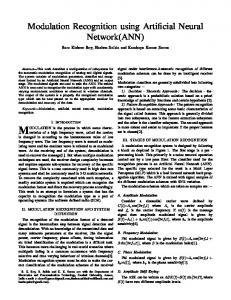
A B C
Figure 1 Representation of the letter A with a form 7 * 5
A grid of 5*7 pixels represents each character. For example, to represent the letter A, we must use the model show in figure (1). Blackened boxes represent a value 1, while empty boxes represent a zero. Can represent all the characters in this way, with a bit map of 35 pixel values. Thus, we used a network with a single layer of 𝑛 = 35 neurons. The parameters used in the stage of learning are: 𝑏 = 0.6, the number of iterations 15, the learning rate 𝜂 = 0.1 and weights initialized randomly between 0 and 0.5. For the 26 alphabets used as a training base, the following results were obtained:
1 0 0 0 … 0 0 0 0 1 0 0 … 0 0 0 0 0 1 0 … 0 0 0
For the parameters we chose the learning rate 𝜂 = 0.75, the number of iterations 116, the weights were initialized randomly between -0.5 and 0.5 the activation function used is the sigmoid. After the end of the learning phase, the following results were obtained:
Figure 4 Square error as a function of the number of iterations (ANN)
Figure 2 Square error as a function of the number of iterations (RNN)
Figure 5 number of alphabets recognized as a function of the number of iterations (ANN)
Figure 3 number of alphabets recognized as a function of the number of iterations (RNN)
B. Application of ANN in alphabets recognition For this application, we used a multi-layer neural network that contains three layers; an input layer has 35 neurons (the number of pixels of the forms used), 8 neurons in the hidden layer, 26 neurons in the last layer. Each character has been identified for output as a vector as the following example shows:
C. Analysis and comparison of the performance of the networks used After having applied the two types of neural networks for recognition of alphabets, we can say that the RNN despite their learning capacity that is faster in terms of number of iterations than ANN, they are (RNN) very expensive in calculations. It suffices to note that at each iteration, we must solve a nonlinear system, of 2𝑛 unknown if we have 𝑛 neurons, and inverting a matrix of size 𝑛 × 𝑛, in our case the used RNN (35 neurons) has become able to recognize all forms in 26 seconds, whereas the ANN used has become able to recognize the same shapes in only 3 seconds. A drawback, which is not always acceptable; especially when working on a large training set or very large (thousands or millions of learning examples) the field of biology, for example. Another drawback of the RNN is their architectures that are generally sets of totally connected neurons, which forces us for network
stability reasons, to work on the basics of learning where each entry has a number of units equal to the number units of its release. Furthermore In addition, the entered must have a binary nature, to be able to be adapted with network inputs (excitatory or inhibitory signals). V.
CONCLUSION
In this work, we have solved an alphabets recognition problem by a random neural network, and a monolayer artificial neural network. The obtained results shows that the RNN despite their high complexity, they have a good learning capacity, against the ANN have good learning ability with low complexity compared to RNN.
REFERENCES [1] [2] [3]
[4] [5] [6]
[7]
E.Gelenbe, (1989), Random neural networks with positive and negative signals and product form solution; Neural Computation, 1, 502 510. E.Gelenbe, (1993), Learning in the recurrent neural network; Neural Computation, 5, 154 164. A.Aguilar, J.Colmenares, (1998), Resolution of pattern recognition problems using a hybrid genetic/random neural network learning algorithm; Pattern Analysis and Applications,1,52 61. S.Timotheou, (2010), The random neural network: a survey; Comput J 53, 251 267. J.Aguilar, C.Molina, (2012), The Multilayer Random Neural Network; Neural Process Lett 37: 111 133. M.Ettaouil and Y.Ghanou, (2009), Neural architectures optimization and Genetic algorithms; Wseas Transactions On Computer, Issue 3, Volume 8, pp. 526 537. M. Ettaouil, Y. Ghanou, K. El Moutaouakil and M. Lazaar,2011,Image Medical Compression by A new Architecture Optimization Model for the Kohonen Networks, International Journal of Computer Theory and Engineering, Vol. 3, No. 2.