Jul 5, 2015 - Bachelor Thesis. Econometrics ... ical programming formulation of the MDVSP in Chapter 4. ... Other mathematical programming approaches.
Solving the multiple-depot vehicle scheduling problem
Bachelor Thesis Econometrics & Operations Research
Nemanja Milovanovi´c 1 Supervisor: Dr. D. Huisman Co-reader: Prof. Dr. A.P.M. Wagelmans
Erasmus School of Economics Erasmus University Rotterdam July 5, 2015
1
Studentnumber: 378244
Abstract The Multiple-Depot Vehicle Scheduling Problem (MDVSP) is the problem where one wants to assign timetabled tasks to vehicles which are housed in multiple depots. This problem is highly relevant for the public transport domain, as competition grows fierce and companies need to stay competitive to survive. As solving the MDVSP optimally is difficult in practice, the aim of this thesis is to give a detailed description for two heuristics discussed in Pepin et al. (2009), namely truncated branch-and-cut and the Lagrangian heuristic. Our implementation of the truncated branch-and-cut heuristic has very poor behavior, which is probably caused by CPLEX’ root node heuristics. Also, in comparison with the heuristics in Pepin et al. (2009), our implementation of the Lagrangian heuristic is rather lackluster, only outperforming their tabu search heuristic. This is probably due to poor code-optimization. Nevertheless, our implementation still provides solutions within 1% optimality gap for all the test instances considered.
i
Contents 1 Introduction
1
2 Problem description
2
3 Literature overview
4
4 Model formulation
5
5 Overview of heuristics 5.1 Truncated branch-and-cut . . . . . . . . . . . . . . . . . 5.2 Lagrangian heuristic . . . . . . . . . . . . . . . . . . . . 5.2.1 Computing the lower bound . . . . . . . . . . . . 5.2.2 Obtaining a feasible solution and an upper bound 5.2.3 An algorithm for the Lagrangian heuristic . . . . 6 Computational results 6.1 Truncated branch-and-cut 6.2 Lagrangian heuristic . . . 6.2.1 Sensitivity analysis 6.2.2 Heuristic results . .
. . . .
. . . .
. . . .
. . . .
. . . .
. . . .
. . . .
. . . .
. . . .
. . . .
. . . .
. . . .
. . . .
. . . .
. . . .
. . . .
. . . .
. . . . .
. . . .
. . . . .
. . . .
. . . . .
7 7 7 7 10 11
. . . .
15 15 16 16 17
7 Conclusion
22
A Forward/reverse auction iterations for the SDVSP
23
B Forward/reverse auction iterations for the AAP
26
ii
1 INTRODUCTION
1
Introduction
As public transport nowadays is getting more and more privatized, firms seek to operate as efficiently as possible in order to attain a better market position. Bus companies and railway operators, for example, all need to create schedules for their vehicles in which is described which trip they cover. This problem is called the vehicle scheduling problem (VSP). In this thesis we will assume that the vehicles are stationed in multiple depots, which is appropriately called the multiple-depot vehicle scheduling problem (MDVSP). The motivation for this thesis is to provide a detailed account on two heuristics discussed in Pepin et al. (2009): Truncated branch-and-cut, and a Lagrangian heuristic. Especially for the Lagrangian heuristic, there are lots of ways to implement the various features. This thesis aims to give the reader an example of which methods can be chosen, and also aims to give a detailed description such that the reader may be able to implement the heuristics himor herself. As such, this thesis is more practically oriented than theoretically. Basic computer and mathematical programming knowledge is assumed. This thesis is organized as follows. In Chapter 2, we describe the MDVSP thoroughly. In Chapter 3, we provide a short overview of the necessary literature used in this thesis and for further reading. We give a mathematical programming formulation of the MDVSP in Chapter 4. Following in Chapter 5, we give an overview of the heuristics which are treated in this paper and we provide the details that are needed to implement them. The computational results of the heuristics are then presented in Chapter 6, after which we conclude this thesis with some remarks in Chapter 7.
1
2 PROBLEM DESCRIPTION
2
Problem description
In this thesis, we base our notation on Pepin et al. (2009). The MDVSP can be described as follows. Given a set T of timetabled tasks and a set of depots K, produce least-cost vehicle schedules in which every task is performed by exactly one vehicle, and the depot capacity vk for k ∈ K is not exceeded. In our case, we assume that all tasks can be performed by vehicles in all depots. This is, for example, the case when the fleet is homogeneous. For every task i ∈ T there exist start and end locations which we model as vertices si and ei , respectively. It is allowed that si = ei , but this need not be the case. Furthermore, a task is characterized by a start time ai ≥ 0, and a duration δi ≥ 0. A vehicle schedule is feasible if all tasks are performed by exactly one vehicle, and for every pair of tasks (i, j) it holds that ai +δi +tij ≤ aj , where tij is the travel time from ei to sj . This implies that task i starts and ends before j does. Total schedule costs are the sum of the total travel and total waiting costs. The total travel costs consists of costs made by traveling from the depot to the first task, traveling in between tasks, and traveling from the last task to the depot. The total waiting costs consist of the sum of the costs of waiting in between tasks. We now introduce some terminology which is quite common in the MDVSP literature. A pull-out trip is a trip from the depot to the start location si of some task i. On the other hand, a pull-in trip is a trip from the end location ei of some task i to the depot. Lastly, a deadhead trip is a trip from the end location ei of task i to the start location sj of task j, for some i 6= j. For an example of an MDVSP (taken from Kliewer et al. 2006), see Figure 1. Here, an instance is depicted with |K| = 2 depots and |T | = 3 tasks, where task 1 starts and ends before task 2, and task 2 starts and ends before task 3. Task i
si
ei
ai
ai + δi
1 2 3
A B B
B A A
1 3 5
2 4 6
Table 1: Example of an MDVSP with |K| = 2 depots and |T | = 3 tasks. There exist several extensions of the MDVSP. A closely related problem is the crew scheduling problem (CSP), which consists of the scheduling of socalled duties. All tasks are assigned to exactly one duty in a cost-minimizing manner, and duties can have additional labor constraints. An extension of the MDVSP is the multiple-depot integrated vehicle- and crew-scheduling problem 2
2 PROBLEM DESCRIPTION
(MD-VCSP) (see Huisman et al. 2005), which integrates the MDVSP with the CSP (normally, CSP and MDVSP are done sequentially). Also, one could consider tasks with time-windows (TW) in the MDVSP or the MD-VCSP, which can considerably lower the necessary amount of vehicles and duties (Kliewer et al., 2012) which in turn lowers the total costs. These extensions will not be considered in this thesis, however.
3
3 LITERATURE OVERVIEW
3
Literature overview
A great starting point in the MDVSP literature is L¨obel (1997), which is a dissertation on optimal vehicle scheduling as applied to public transit. This dissertation focuses primarily on the MDVSP, more specifically, it provides a short overview of the necessary mathematics involved after which several techniques are discussed to solve the MDVSP exactly, including branch-andbound and variants thereof. Other mathematical programming approaches can be found in Hadjar et al. (2006), and Ribeiro and Soumis (1994). Although the MDVSP is often formulated as a connection network, Kliewer et al. (2006) apply the time-space network model to the problem. Also, because of this modeling approach, they are able to aggregate many deadhead arcs. The authors report a tremendous reduction in variables due to this aggregation. As the MDVSP is NP-hard, several heuristic approaches have been proposed. An overview of some heuristics can be found in Pepin et al. (2009). Also, they propose a large neighborhood search (LNS) heuristic which uses column generation to evaluate the neighborhood. More recently, other local search heuristics have been proposed by Laurent and Hao (2009) and Otsuki and Aihara (2014). The former propose an iterated local search heuristic (ILS) which uses the notion of ejection chains in the construction of their neighborhood. The latter present a variable-depth local search heuristic (VDS), which utilizes the previous ILS in a variable-depth context. Both articles use the same test instances as presented in Pepin et al. (2009) and report superior results as compared to their LNS (still inferior to their column generation approach), but fail to compare computation times. The Lagrangian heuristic as discussed in this paper uses three key features that require additional literature. First and foremost, it uses subgradient optimization to optimize the Lagrangian multipliers. Although this thesis uses the subgradient method proposed by Pepin et al. (2009), the reader may find it useful to try a different method. We therefore point the reader to a dissertation by Guta (2003), in which subgradient optimization is treated extensively. The second and third features are obtaining the lower and upper bounds, respectively. For these components, we use auction algorithms as proposed by Freling et al. (2001) and Bertsekas and Casta˜ non (1992) for the quasi-assignment and asymmetric assignment problems, respectively. Alternatives to these auction algorithms can also be used. Some of these can be found in the book by Bertsekas (1998), which is an excellent account on network optimization in general.
4
4 MODEL FORMULATION
4
Model formulation
The MDVSP can be formulated in different ways. However, in this thesis we only use one formulation, namely the connection network variant of the multi-commodity flow network, which can be described as follows. Let Gk = (V k , Ak ) for each depot k ∈ K. Here V k is the set of vertices, which contains each task vertex i ∈ T and also o(k) and d(k), respectively the start and end vertices of depot k. Thus, it holds that V k = {o(k), d(k)}∪T . The set of arcs Ak contains three types of arcs: pull-out arcs, connection arcs, and pull-in arcs. Pull-out arcs are defined as pairs (o(k), j) for all j ∈ T . This means that every task has a pull-out arc connected with it. Similarly, all tasks also have a pull-in arc which is defined as (i, d(k)) for all i ∈ T . Finally, there are connection arcs. These arcs are characterized as (i, j), where i, j ∈ T , connecting two task i and j such that ai +δi +tij ≤ aj . The last parameter in the model is the cost of an arc, which we denote by cij . This cost is usually equal to the travel costs between tasks i and j, but other costs are also allowed. For instance, if i = o(k) then it is possible that a certain fixed-cost is incurred.
o(1)
1
2
3
d(1)
o(2)
1
2
3
d(2)
pull-in/out arc
connection arc
Figure 1: Example from Table 1 modeled as a connection network. Here, circular vertices represent tasks and rectangular vertices are associated to depots. For an example of the connection network approach, see Figure 1, which extends the example from Table 1. Note that every depot has its own network layer and that the cost of arc (i, j) does not necessarily have to be the same between depots. We are now ready to present the connection network flow formulation as
5
4 MODEL FORMULATION
presented by Pepin et al. (2009) for the MDVSP, which is as follows: X X min cij Xijk
(1)
k∈K (i,j)∈Ak
s.t.
X
X
k∈K
j:(i,j)∈Ak
X
Xijk = 1,
∀i ∈ T,
k Xo(k),j ≤ vk ,
(2)
∀k ∈ K,
(3)
j:(o(k),j)∈Ak
X
Xjik −
j:(j,i)∈Ak
Xijk ∈ B,
X
Xijk = 0,
∀i ∈ V k \ {o(k), d(k)}, k ∈ K, (4)
∀(i, j) ∈ Ak , k ∈ K,
(5)
j:(i,j)∈Ak
where B = {0, 1}, and vk is the vehicle capacity of depot k. Also, Xijk are the decision variables of this model which equal 1 if arc (i, j) ∈ Ak has flow coming from depot k and 0 otherwise. Flow in this context can be seen as a vehicle traveling from task i to task j. Objective function (1) minimizes the total costs. Constraints (2) ensure that every task is performed by exactly one vehicle, while constraints (3) keep the number of dispatched vehicles from depot k below the corresponding capacity. Lastly, constraints (4) conserve the flow through all nodes, as all incoming flow through a certain task vertex must also go out.
6
5 OVERVIEW OF HEURISTICS
5 5.1
Overview of heuristics Truncated branch-and-cut
When one incorporates cutting planes (see Gomory, 1963) in a brand-andbound algorithm, the result is known as branch-and-cut. As this subject is not in the scope of this text, we refer the interested reader to Mitchell (2002). As letting the branch-and-cut algorithm run to completion is too time consuming for large problem instances, we could simply terminate the algorithm after the first feasible integer solution we find. This results in a procedure which is called truncated branch-and-cut. This procedure is actually a heuristic, as we are not guaranteed that the solution we find is optimal. For the branch-and-cut implementation we use the connection network formulation, which was discussed in Chapter 4, and we implement it using the commercial MIP solver CPLEX (version 12.6, 32-bits), with default settings unless stated otherwise.
5.2
Lagrangian heuristic
A Lagrangian heuristic is a heuristic which uses a Lagrangian relaxation to obtain lower bounds for the problem at hand. Usually, an upper bound is obtained by “transforming” the lower bound solution to a feasible one. Lagrangian relaxation transfers certain constraints to the objective function by introducing new variables called Lagrangian multipliers. The problem of assigning these multipliers values such that the lower bound is as tight as possible is called the Lagrangian dual problem. Additionally, the objective function to the Lagrangian dual problem is called the Lagrangian dual function. As the Lagrangian dual function is non-smooth, a popular choice in solving the dual problem is subgradient optimization. For a more detailed text on subgradient optimization for the Lagrangian dual problem with applications, we refer the reader to Guta (2003). This section outlines the heuristic proposed by Pepin et al. (2009). In the following, we provide the reader with details regarding every aspect of the Lagrangian heuristic. 5.2.1
Computing the lower bound
As described earlier, the Lagrangian dual problem is obtained when one relaxes certain constraints. However, there is no limit on the choice of which constraints to relax. The Lagrangian heuristic is based on the connections network formulation given by (1)–(5) augmented by the redundant
7
5.2 Lagrangian heuristic
5 OVERVIEW OF HEURISTICS
constraints: X
X
k∈K
j:(j,i)∈Ak
Xjik = 1,
∀i ∈ T.
(6)
The Lagrangian dual problem is then obtained by relaxing constraints (3) by deleting them, and relaxing constraints (4) in a Lagrangian fashion, as follows: X X φ(λ) = min c˜ij Xijk (7) k∈K (i,j)∈Ak
s.t.
X
X
k∈K
j:(i,j)∈Ak
X
X
Xijk = 1,
∀i ∈ T,
(8)
Xjik = 1,
∀i ∈ T,
(9)
k∈K j:(j,i)∈Ak
Xijk ∈ B,
∀(i, j) ∈ Ak , ∀k ∈ K,
(10)
∀i, j ∈ T ∀j ∈ T, i = o(k) . ∀i ∈ T, j = d(k)
(11)
where c˜ij is defined as k k cij + λj − λi c˜ij = cij + λkj cij − λki
This dual problem is equivalent to a single-depot vehicle scheduling problem (SDVSP), which can be seen by replacing Xijk with a single variable corresponding to the arc (i, j) for which cij + λkj − λki is the lowest. This SDVSP can be solved in a manner of ways (see Freling et al. 2001), one of which is an auction algorithm. An auction algorithm in the SDVSP sense is an algorithm in which tasks bid for other tasks or the start/end vertices of the depot. The auction algorithm Freling et al. (2001) proposed for the SDVSP consists of forward and reverse auction iterations. In a forward iteration, trips bid for successor trips or the end vertex of the depot, and in a reverse iteration trips bid for predecessor trips or the start vertex of the depot. The pseudo-code for both types of iteration can be found in Appendix A. In the combined forward and reverse auction algorithm as proposed by Freling et al. (2001), one switches between forward and reverse iterations. Freling et al. (2001) also guarantees convergence when one refrains from switching between the iterations until at least one more task is forward or backward assigned. Also, the start values of the dual variable vectors π and p may be chosen arbitrarily. 8
5.2 Lagrangian heuristic
5 OVERVIEW OF HEURISTICS
In theory, the previously described algorithm should always terminate. However, in practice we see that if ε < |T1 | remains constant during the auction algorithm, it may take many iterations before the algorithm converges. Luckily, one can remedy this by means of ε-scaling. ε-scaling is a technique where the original problem is solved several times for decreasing values of ε according to some (monotonically) decreasing function f (ε, i), where i is the number of the iteration, until finally ε < |T1 | , in which case the solution is optimal. Freling et al. (2001) proposes the following updating scheme. First, for all (i, j) we define new costs a0ij = |T +1|aij . Then, we define the ε-scaling function to be f (ε, i) = max{1, ∆/θi }, (12) with ∆ = |T | max(i,j) |a0ij | and θ = 4. The new optimality criterion for the auction algorithm then becomes ε = 1. The entire auction procedure (including ε-scaling) can be found in Algorithm 1. Algorithm 1 The entire auction algorithm for the SDVSP. 1: procedure Auction 2: ε ← initial value 3: π ← 0, p ← 0 4: i←1 5: do forward ← true 6: while ε > 1 do 7: S←∅ 8: while ∃i, j ∈ T : (i, j) 6∈ S do 9: if ∃i ∈ T : (i, j) 6∈ S and do forward is true then 10: forward(p, π, ε, S) 11: if we forward assigned, do forward is false 12: end if 13: if ∃j ∈ T : (i, j) 6∈ S and do forward is false then 14: reverse(p, π, ε, S) 15: if we backward assigned, do forward is true 16: end if 17: end while 18: i←i+1 19: ε ← f (ε, i) 20: end while 21: return S 22: end procedure
9
5.2 Lagrangian heuristic
5.2.2
5 OVERVIEW OF HEURISTICS
Obtaining a feasible solution and an upper bound
The next step in the heuristic is obtaining an upper bound to the original problem. Although several options are possible, usually the solution corresponding to the lower bound is made feasible using some procedure. In our case, we have obtained a number of paths which are assigned to a single depot. By assigning these paths to different depots and keeping in mind the capacity constraints, we obtain a feasible solution for the MDVSP. Formally, we have the following problem: XX min ckp Ypk (13) k∈K p∈P
s.t.
X
Ypk = 1,
∀p ∈ P,
(14)
k∈K
X
Ypk ≤ vk ,
∀k ∈ K,
(15)
p∈P
Ypk ∈ B,
∀p ∈ P, ∀k ∈ K,
(16)
where P is the set of all paths obtained by solving the Lagrangian subproblem, and K is the set of depots. Also, ckp is the cost of letting path p be serviced by a vehicle from depot k, and vk is the capacity for depot k. Furthermore, the decision variable Ypk is equal to 1 if path p is serviced from depot k, and 0 otherwise. The objective function (13) minimizes the total costs, constraints (14) make sure that every path is serviced by exactly one depot, and constraints (15) guarantee that the depot capacities are respected. The problem described by (13)–(16) is called a transportation problem and can be solved by a variety of methods. In this thesis, we propose to solve the transportation problem by transforming it into an asymmetric assignment problem (AAP), which we solve by means of a combined forward and reverse auction algorithm proposed by Bertsekas and Casta˜ non (1992). More information about the forward/reverse iterations can be found in Appendix B. The transformation is simple, we split every depot k ∈ K into vk artificial depots. We denote the set of artificial depots by K 0 , which has
10
5.2 Lagrangian heuristic cardinality |K 0 | =
P
k∈K
5 OVERVIEW OF HEURISTICS
vk . The resulting AAP then becomes:
min
XX
ckp Ypk
(17)
k∈K 0 p∈P
s.t.
X
Ypk = 1,
∀p ∈ P,
(18)
Ypk ≤ 1,
∀k ∈ K 0 ,
(19)
∀p ∈ P, ∀k ∈ K 0 .
(20)
k∈K 0
X p∈P
Ypk ∈ B,
Note that instead ofP having |K||P | variables using the transportation problem, we now have k∈K vk |P | ≥ |K||P | variables. This shows that the complexity of the auction algorithm (which is dependent on the number of variables) will be heavily influenced by the depot capacities. However, transformations done on the data instances which will be introduced in Chapter 6 showed that the number of paths |P | remains relatively small, and so the transformed transportation problem, even for rather large instances (|T | = 1500), is solved swiftly. As with the SDVSP auction algorithm, it is possible to achieve convergence faster with ε-scaling. We let the scaling function f (ε, i) be the same as before, where we define ∆ as ∆ = |P | max(p,k) |a0pk | and a0pk = |P + 1|apk . The complete auction procedure can be found in Algorithm 2. 5.2.3
An algorithm for the Lagrangian heuristic
Now for the final ingredient for the Lagrangian heuristic: the subgradient optimization procedure. As already mentioned, the Lagrangian dual function is non-smooth, so optimization by means of gradient descent methods is out of the question. For this reason, one often turns to subgradient optimization, as subgradients are available even for non-differentiable points. The basic form of a subgradient procedure is λk,n+1 = λk,n + δn sk,n i i i ,
(21)
where λk,n is the Lagrangian multiplier of iteration n, δn is a scalar, and sk,n i i is a subgradient. Note that subgradient optimization comes in many flavors, of which in this thesis we only focus on the one suggested by Pepin et al.
11
5.2 Lagrangian heuristic
5 OVERVIEW OF HEURISTICS
Algorithm 2 The complete auction procedure for solving the AAP. procedure AsymmetricAuction ε ← initialvalue π ← 0, p ← 0 λ ← 0, i ← 0 while ε > 1 do S ← ∅ forward() λ ← mink:(p,k)∈S pk do forward ← true while there is an unassigned p ∈ P and ∃k ∈ K 0 : pk ≤ λ do if do forward is true then forward(p, π, ε, S, λ) if we forward assigned, do forward is false end if if do forward is false and ∃k ∈ K 0 : pk ≤ λ then reverse(p, π, ε, S, λ) if we backward assigned, do forward is true if all p ∈ P are assigned, do forward is false end if end while i←i+1 ε ← f (ε, i) end while end procedure
12
5.2 Lagrangian heuristic
5 OVERVIEW OF HEURISTICS
(2009), namely: U B − φ(λn ) , P k,n 2 k∈K i∈T (si ) X X Xjik,n − Xijk,n ,
δn = αn P sk,n = i
j:(j,i)∈Ak
(22) (23)
j:(i.j)∈Ak
where U B is the best upper bound found so far, α0 is left as a parameter to be chosen by the user, and the rule for updating αn+1 given αn will be given shortly. The entire Lagrangian heuristic (as suggested by Pepin et al. 2009) is given in Algorithm 3. First, we compute a lower bound φ(λn ) by solving the Lagrangian subproblem given a vector λn of Lagrangian multipliers. Then, we make this (often unfeasible) solution feasible for the MDVSP by transforming it. We do this by means of solving a transportation problem. Then, we update the lower and upper bounds, and the Lagrangian multipliers using a subgradient optimization procedure. Finally, we check if we fulfilled a stopping criterium, and if so, we terminate the heuristic. If not, we begin by computing a new lower bound, and so on. Also, we use the following updating rule for αn . Every γ iterations in which we have not improved our lower bound, we halve αn . The stopping criteria we use are the following. If the upper and lower bounds collide, we stop as we have found the optimal solution. Also, if αn is too small, say smaller than ε, or after nmax iterations, we terminate the procedure.
13
5.2 Lagrangian heuristic
5 OVERVIEW OF HEURISTICS
Algorithm 3 Lagrangian heuristic for solving the MDVSP. 1: 2: 3: 4: 5: 6: 7: 8: 9: 10: 11: 12: 13: 14: 15: 16: 17: 18: 19: 20: 21: 22: 23: 24: 25: 26: 27: 28: 29: 30:
procedure LagrangianHeuristic(nmax , γ, ε) U B ← ∞, LB ← −∞ n ← 0, m ← 0, λ0 ← 0 while true do solve Lagrangian subproblem (7)–(10) to obtain Xn and φ(λn ) compute a subgradient sk,n i compute an upper bound U Bn by solving (13)–(16) if U Bn < U B then U B ← U Bn end if λk,n+1 = λk,n + δn sk,n i i i if φ(λn ) > LB then m←0 LB ← φ(λn ) else m←m+1 end if if m = γ then αn+1 ← αn /2 m←0 else αn+1 ← αn end if if U B = LB, αn ≤ ε, or n ≥ nmax then stop else n←n+1 end if end while end procedure
14
6 COMPUTATIONAL RESULTS
6
Computational results
All results were obtained with a computer running Windows 7 (64-bit) with Intel Core i7-4770 CPU at 3.40GHz and 8GB RAM. Additionally, we used Java (version 1.8.0u45, 32-bits) to program (parts of) the heuristics. In case a MIP solver was necessary, we used the commercial MIP solver CPLEX (version 12.6, 32-bits). All user-created code runs on a single thread. The test instances we used in this thesis to evaluate the heuristics were created by Pepin et al. (2009) and are available from http://people.few. eur.nl/huisman/instances.htm. Optimal costs and optimal amount of vehicles can also be found here. The data vary in two dimensions, namely number of depots and number of tasks. Also, for every depot-task pair, there are five different cases available. Table 2 gives the reader an insight in how big the test instances are. Here, we have summed the number of arcs across all depots. Table 2: Number of arcs for the 500, 1000, and 1500 task test instances, for both 4 and 8 depots. Instance
500 tasks
1000 tasks
1500 tasks
0 1 2 3 4
304,620 307,728 311,772 307,676 301,868
1,221,640 1,224,572 1,218,576 1,194,052 1,207,288
2,684,272 2,763,400 2,744,656 2,757,136 2,750,936
(a) 4-depot case
Instance
500 tasks
1000 tasks
1500 tasks
0 1 2 3 4
615,488 624,744 620,208 611,640 615,672
2,435,368 2,477,024 2,412,984 2,422,160 2,389,192
5,453,944 5,459,040 5,486,792 5,514,720 5,534,336
(b) 8-depot case
6.1
Truncated branch-and-cut
Before we present the results obtained from the truncated branch-and-cut heuristic, we should mention that using the 32-bits version of CPLEX has 15
6.2 Lagrangian heuristic
6 COMPUTATIONAL RESULTS
severe drawbacks regarding solving the MDVSP. Due to the relatively large amount of memory CPLEX needs for the MDVSP, it is impossible to solve the larger test instances; we were only able to solve the instances with 4 depots and 500 tasks. Also, selecting any algorithm other than the barrier algorithm at the root node lead to memory problems. Table 3: Results of the truncated branch-and-cut heuristic for the test instances of category “4 depots, 500 tasks”. The optimality gap is calculated using the optimal costs. Instance
Gap (%)
Time (s)
Absolute costs
0 1 2 3 4
49.33 50.44 46.10 50.24 44.30
20.45 21.34 22.12 20.74 22.51
2,544,110 2,505,449 2,381,940 2,529,575 2,364,573
The results of the truncated branch-and-cut are shown in Table 3. The reported optimality gap is calculated with Gap =
100(U B − LB) . UB
(24)
We see from the table that using the first obtained solution results in optimality gaps which are quite large. This can be explained by CPLEX’ default behavior. When left default, CPLEX uses heuristics at the root node which give quick solutions. The quality of these quick solutions, however, may turn out be poor, as is likely our case. To investigate this, one could turn off these root node heuristics. Unfortunately, when doing so, we ran into memory problems, which prohibited us to investigate this issue any further.
6.2 6.2.1
Lagrangian heuristic Sensitivity analysis
As there is quite some freedom in choosing the parameters for the subgradient procedure described in Chapter 5.2.1, we begin with a small sensitivity analysis. As a reference point, we take the following parameter values: nmax = 500, α0 = 1.0, γ = 10, ε = 0.000001. Also, due to the fact that sensitivity analysis requires many runs of the algorithm, we limit ourselves to the 4-depot instances with 500 tasks and assume that the larger instances comply in behavior. 16
6.2 Lagrangian heuristic
6 COMPUTATIONAL RESULTS
We vary the parameters α0 and γ, which both give us some control over the size of the step we take in the direction of the subgradient. Setting the parameter α0 relatively large (small) results in taking relatively big (small) steps in the direction of the subgradient, whereas assigning γ a large (small) value leads to relatively slow (fast) decline of the step size. In this sensitivity analysis we consider the values α0 = 0.5, 0.8, 1.0, 1.5 and γ = 1, 3, 5, 7, 10, 15. The results of which can be found in Figure 2 and Figure 3. From the two figures it is obvious that there exist trade-offs for both parameters, where the trade-off for α0 is the most apparent. In both cases we find that an increase in solution quality requires an increase in computation time. 6.2.2
Heuristic results
Considering the results of the sensitivity analysis, we ultimately decide upon the following parameter values: nmax = 500, α0 = 1.0, γ = 7, ε = 0.000001. Next, we would like to visually summarize the proposed Lagrangian heuristic by means of Figure 4. In this figure, which was made by applying the heuristic to an instance with four depots and 1500 tasks, we see that the lower bound increases non-monotonically, which is typical for subgradient methods. Nevertheless, the lower bound does seem to converge to a particular value. Also interesting to note is that the upper bound seems to have a tendency to decrease. Small experiments have shown that the quality of the upper bound tends to the quality of the lower bound. Which means that if the lower bound is of poor quality, the upper bound also tends to be poor. Our last observation is that looking at the best available upper bounds, we see that after a certain number of iterations, it is not very rewarding to let the heuristic continue. Finally, using the aforementioned parameter values, we run the Lagrangian heuristic for all test instances and compare the results with the heuristics in Pepin et al. (2009). In accordance to Pepin et al. (2009), we subtract the fixed vehicle costs from the objective value and use the result for comparison purposes. Table 4 and Table 5 show the results of the comparison for the 4-depot and 8-depot instances. The abbreviations for the heuristics are as follows: – CLGR: Column generation; – LGRH: Lagrangian heuristic. Note that Pepin et al. (2009) use an unknown method to solve the transportation problem; – LNS: Large neighborhood search; – TBnC: Truncated branch-and-cut; 17
6.2 Lagrangian heuristic
1.2798
6 COMPUTATIONAL RESULTS
×10 6
1.2798 1.2797
Costs
1.2797 1.2796 1.2796 1.2795 1.2795 1.2794 0.5
0.6
0.7
0.8
0.9
1
1.1
1.2
1.3
1.4
1.5
1.1
1.2
1.3
1.4
1.5
α
(a) 386 384 382
Time
380 378 376 374 372 370 368 0.5
0.6
0.7
0.8
0.9
1
α
(b)
Figure 2: Graphs where various values for α0 are plotted against (a) mean total costs, and (b) mean computation time in seconds. For both graphs, the mean is taken over the five instances with four depots and 500 tasks.
18
6.2 Lagrangian heuristic
1.2812
6 COMPUTATIONAL RESULTS
×10 6
1.281 1.2808 1.2806
Costs
1.2804 1.2802 1.28 1.2798 1.2796 1.2794 1.2792 0
5
10
15
10
15
γ
(a) 400
350
Time
300
250
200
150
100
50 0
5
γ
(b)
Figure 3: Graphs where various values for γ are plotted against (a) mean total costs, and (b) mean computation time in seconds. For both graphs, the mean is taken over the five instances with four depots and 500 tasks.
19
6.2 Lagrangian heuristic
3.6
6 COMPUTATIONAL RESULTS
×10 6 Lower bound Upper bound Best upper bound Best available solution
3.595 3.59 3.585
cost
3.58 3.575 3.57 3.565 3.56 3.555 3.55 0
50
100
150
200
250
300
350
400
450
500
iteration
Figure 4: Typical behavior of the Lagrangian heuristic. This graph was made applying the heuristic on an instance with four depots and 1500 tasks. Table 4: Average best scaled solutions for the 4-depot instances. The best scoring heuristic is used as reference. 500 tasks
1000 tasks
1500 tasks
Heuristic
Time (s)
Objective
Time (s)
Objective
Time (s)
Objective
CLGR LGRH∗ LGRH LNS TBnC TS
77 85 85 85 81 85
1.0000 1.0535 1.0294 1.0201 1.0013 1.1073
651 700 700 700 1287 700
1.0016 1.0408 1.0370 1.0124 1.0000 1.0812
2203 2300 2300 2300 4149 2300
1.0019 1.0536 1.0531 1.0182 1.0000 1.1054
∗
: Own implementation
20
6.2 Lagrangian heuristic
6 COMPUTATIONAL RESULTS
Table 5: Average best scaled solutions for the 8-depot instances. The best scoring heuristic is used as reference. 500 tasks
1000 tasks
1500 tasks
Heuristic
Time (s)
Objective
Time (s)
Objective
Time (s)
Objective
CLGR LGRH∗ LGRH LNS TBnC TS
119 125 125 125 612 125
1.0000 1.0770 1.0494 1.0262 1.0014 1.1722
857 900 900 900 6207 900
1.0091 1.0960 1.0597 1.0265 1.0000 1.1896
3085 3200 3200 3200 – 3200
1.0000 1.1021 1.0923 1.0283 – 1.1981
∗
: Own implementation – TS: Tabu search.
The truncated branch-and-cut has no value for the 8-depot cases with 1500 tasks, because it failed to find a solution within 10 hours computation time for some of the instances. We have omitted our implementation of the truncated branch-and-cut heuristic because of the extremely poor performance. For all test instances we have adopted the same run times as Pepin et al. (2009), for fair comparison. As such, for the 4-depot case, our heuristic ran for 85, 125, and 700 seconds for the 500, 100, and 1500 task instances, respectively. For the 8-depot case, these run times are 125, 900, and 3200 seconds. From Table 4 and Table 5 we can conclude that performance-wise, our implementation of the Lagrangian heuristic is outperformed by all other heuristics, except tabu search. As our implementation has quite different performance as compared to the implementation by Pepin et al. (2009), and the fact that the machine used in this thesis is more powerful, we must conclude that our implementation is poorly optimized.
21
7 CONCLUSION
7
Conclusion
In this thesis we gave a detailed account on two heuristics based on mathematical programming techniques which can be used to solve the MDVSP. Although the truncated branch-and-cut heuristic does not provide acceptable solutions, we think this is caused by the root node heuristics implemented in CPLEX. For the Lagrangian heuristic, we have thoroughly described methods to solve the Lagrangian dual problem and how to transform a solution of such problem to a feasible solution for the MDVSP. Note that other methods may be used. For instance, one could opt to solve the Lagrangian dual problem with CPLEX, or another method could be used to transform the solution of the dual problem. Comparing the results of our implementation of the Lagrangian heuristic to heuristics proposed by Pepin et al. (2009), we see that ours is rather lackluster, beating only the tabu search heuristic in terms of solution quality. This lackluster performance is most likely caused by poor optimization of the code. This does not mean that our implementation is not suited for practical issues, as the optimality gap (not subtracting fixed-costs) does not exceed 1% for all test instances considered.
22
A FORWARD/REVERSE AUCTION ITERATIONS FOR THE SDVSP
A
Forward/reverse auction iterations for the SDVSP
This appendix is dedicated to give a thorough enough description of the forward and reverse auction iterations for implementation purposes. For the validity of the upcoming algorithms we refer the reader to Freling et al. (1997). First we introduce some terminology. Let the set of all arcs in the SDVSP be A. Let A(i) = {j : (i, j) ∈ A, j ∈ T ∪ d}, where d is the end vertex of the depot, be the set of successor vertices of i. Similarly, let B(j) = {i : (i, j) ∈ A, i ∈ T ∪ o}, where o is the start vertex of the depot, be the set of predecessor vertices of j. As is custom with auction terminology, we consider the SDVSP as a maximization problem by replacing the costs cij with aij = −cij . Also, when (i, j) ∈ A is included in the solution, we call i and j forward and backward assigned, respectively. Next, let π and p be vectors of dual variables corresponding to the linear assignment formulation of the SDVSP. In auction terminology πi is the vector of profits of forward assigning task i and pj is the price of backward assigning task j. Finally, let fij = aij − pj where i and j are both tasks, and let fid = aid + ε, where ε > 0. Here, fij represents the amount task i bids for task j. It can be shown that when ε < |T1 | , the auction algorithm terminates with the optimal solution. Pseudo-code for the forward auction iteration can be seen in Algorithm A.1. For the reverse auction there are some small changes, but the main idea stays the same. Task j now makes a reverse bid rij = aij −πi where i is a task, and roj = aoj + ε where o is the start vertex of the depot. The pseudo-code for the reverse auction iteration is depicted by Algorithm A.2.
23
A FORWARD/REVERSE AUCTION ITERATIONS FOR THE SDVSP
Algorithm A.1 Algorithm for the forward auction iteration. 1: 2: 3: 4: 5: 6: 7: 8: 9: 10: 11: 12: 13: 14: 15: 16: 17: 18: 19: 20:
procedure Forward(p, π, ε, S) for i ∈ T : (i, j) 6∈ S do ji ← arg maxj∈A(i) fij βi ← fiji if |A(i)| > 1 then γi ← maxj∈A(i),j6=ji fij else γi ← −∞ end if if ji 6= d then pji ← pji + βi − γi + ε = aiji − γi + ε πi ← aiji − pj S ← S ∪ (i, ji ) if ji already assigned, then remove that assignment else πi ← aid S ← S ∪ (i, d) end if end for end procedure
24
A FORWARD/REVERSE AUCTION ITERATIONS FOR THE SDVSP
Algorithm A.2 Algorithm for the reverse auction iteration. 1: 2: 3: 4: 5: 6: 7: 8: 9: 10: 11: 12: 13: 14: 15: 16: 17: 18: 19: 20:
procedure Reverse(p, π, ε, S) for j ∈ T : (i, j) 6∈ S do ij ← arg maxi∈B(j) rij βj ← f ij j if |B(j)| > 1 then γj ← maxi∈B(j),i6=ij rij else γj ← −∞ end if if ij 6= o then πij ← πij + βj − γj + ε = aij j − γj + ε p j ← ai j j − π i S ← S ∪ (ij , j) if ij already assigned, then remove that assignment else pj ← aoj S ← S ∪ (o, j) end if end for end procedure
25
B FORWARD/REVERSE AUCTION ITERATIONS FOR THE AAP
B
Forward/reverse auction iterations for the AAP
The auction iterations used in this thesis for the AAP are very much alike the ones in Appendix A. We therefore refer the reader to Appendix A for the relevant notation. The following forward and reverse auction iterations are proposed by Bertsekas (1998). They are only adapted in terms of notation. Let a forward bid be defined as fpk = apk − pk where apk = −ckp , p is path, and k is a depot. This means that in this case, paths bid on depots. Similarly, a reverse bid is defined as rpk = apk − πp , where similarly depots bid on paths. Furthermore, we introduce a new scalar, defined after one forward iteration as λ = mink:(p,k)∈S pk . Finally, the optimality criterion in this case becomes ε < |P |. The entire forward and reverse iterations can be found in Algorithm B.1 and Algorithm B.2 Algorithm B.1 Forward auction iteration for the asymmetric assignment problem. 1: 2: 3: 4: 5: 6: 7: 8: 9: 10: 11: 12: 13: 14: 15: 16: 17:
procedure Forward(p, π, ε, S, λ) for p ∈ P : (p, k) 6∈ S do kp ← arg maxk∈A(p) fpk βp ← fpkp if |A(p)| > 1 then γp ← maxk∈A(p),k6=kp fpk else γp ← −∞ end if pk ← max{λ, apkp − γp + ε} πp ← γp − ε if λ ≤ apkp − γp + ε then S ← S ∪ (p, kp ) if k was already assigned, remove that assignment from S end if end for end procedure
26
B FORWARD/REVERSE AUCTION ITERATIONS FOR THE AAP
Algorithm B.2 Reverse auction iteration for the asymmetric assignment problem. 1: 2: 3: 4: 5: 6: 7: 8: 9: 10: 11: 12: 13: 14: 15: 16: 17: 18: 19: 20: 21:
procedure Reverse(p, π, ε, S, λ) for k ∈ K : (p, k) 6∈ S, pk > λ do pk ← arg maxp∈B(k) rpk βk ← rkp p if |B(k)| > 1 then γk ← maxp∈B(k),p6=pk rpk else γk ← −∞ end if if λ ≥ βk − ε then pk ← λ continue else δ ← min{βk − λ, βk − γk + ε} pk ← βk − δ πpk ← πpk + δ S ← S ∪ (pk , k) if p was already assigned, remove that assignment from S end if end for end procedure
27
REFERENCES
REFERENCES
References D.P Bertsekas. Network Optimization: Continuous and Discrete Models. Athena Scientific, 1998. D.P Bertsekas and D.A Casta˜ non. A Forward/Reverse Auction Algorithm for Asymmetric Assignment Problems. Computational Optimization and Applications, 1, 1992. R. Freling, A.P.M. Wagelmans, and J.M.P. Paix˜ao. Models and Algorithms for Vehicle Scheduling. Working paper, 1997. R. Freling, A.P.M. Wagelmans, and J.M.P. Paix˜ao. Models and Algorithms for Single-Depot Vehicle Scheduling. Transportation Science, 35(2), 2001. R.E. Gomory. An algorithm for integer solutions to linear programs. In R.L Graves and P. Wolfe, editors, Recent advances in mathematical programming. McGraw-Hill, 1963. B. Guta. Subgradient Optimization Methods in Integer Programming with an Application to a Radiation Therapy. PhD thesis, Technische Universit¨at Kaiserslautern, 2003. A. Hadjar, O. Marcotte, and F. Soumis. A Branch-and-Cut Algorithm for the Multiple Depot Vehicle Scheduling Problem. Operations Research, 54 (1), 2006. D. Huisman, R. Freling, and A.P.M. Wagelmans. Multiple-Depot Integrated Vehicle and Crew Scheduling. Transportation Science, 39(4), 2005. N. Kliewer, T. Mellouli, and L. Suhl. A time-space network based exact optimization model for multi-depot bus scheduling. European Journal of Operational Research, 175, 2006. N. Kliewer, B. Amberg, and B. Amberg. Multiple depot vehicle and crew scheduling with time windows for scheduled trips. Public Transport, 3, 2012. B. Laurent and J-K. Hao. Iterated local search for the multiple depot vehicle scheduling problem. Computers & Industrial Engineering, 57:277–286, 2009. A. L¨obel. Optimal Vehicle Scheduling in Public Transit. PhD thesis, Technische Universit¨at Berlin, 1997. 28
REFERENCES
REFERENCES
J.E. Mitchell. Branch-and-Cut Algorithms for Combinatorial Optimization Problems. In P.M. Pardalos and M.G.C. Resende, editors, Handbook of Applied Optimization, pages 65–77. Oxford University Press, 2002. T. Otsuki and K. Aihara. New variable depth local search for multiple depot vehicle scheduling problems. Journal of Heuristics, 2014. A. Pepin, G. Desaulniers, A. Hertz, and D. Huisman. A comparison of five heuristics for the multiple depot vehicle scheduling problem. Journal of Scheduling, 12:17–30, 2009. C.C. Ribeiro and F. Soumis. A column generation approach to the multipledepot vehicle scheduling problem. Operations Research, 42, 1994.
29