2011 IEEE/RSJ International Conference on Intelligent Robots and Systems September 25-30, 2011. San Francisco, CA, USA
Sound Source Localization for Mobile Robot Based on Time Difference Feature and Space Grid Matching Xiaofei Li, Hong Liu∗ and Xuesong Yang Abstract— Auditory is a convenient and efficient way for Human-Robot Interaction, however implementing a sound source localization system based on TDOA method encounters many problems, such as noise of real environments, and resolution of nonlinear equations, switch between far field and near field and lack of microphones for geometric positioning localization method. In this paper, a new spectral weighting GCC-PHAT method is proposed to deal with noise. Furthermore, the time difference feature of sound source and its spatial distribution are analyzed. Based on prosperities of the distribution, a space grid matching (SGM) algorithm is proposed for localization step, which handles those problems that geometric positioning method faces effectively. Decision tree and valid feature detection algorithm are also proposed to reduce computational complexity and improve performance. Experiments are achieved in real environments on a mobile robot platform, in which 2016 sets of speech data are tested using four microphones in 3D space. More than 95% azimuth localization rate with error less than 5 degrees and approximate 90% horizontal distance localization rate are obtained.
I. INTRODUCTION Auditory system is constructed for friendly Human-Robot Interaction (HRI) because of its naturalness and effectiveness. More attentions were paid into auditory functions for robots including sound source localization and separation, automatic speech recognition, speaker recognition and so on in last decades. Sound source localization (SSL) for HRI means that the robot can compute the location of sound source through sound signals collected by microphone array fixed on the robot, where sound signal is speech in most cases. Irie from MIT installed a simple auditory system for robots in 1995 [1]. Q.H. Wang from Toronto University presented a SSL system for robot localization and navigation based on SRP-PHAT (steered response power-phase transformation) algorithm [2]. Jonas H. implemented a SSL system for humanoid robots based on two microphones [3]. Honda Co. stated an open source software system for robot audition HARK consisted of sound source localization, separation and speech recognition [4]. Carlos T.Ishi evaluated a MUSICbased real-time sound localization of multiple sound sources in real noisy environments [5]. XiaoFei Li is with the Key Laboratory of Integrated Micro-system, Shenzhen Graduate School, Peking University, Shenzhen, 518055, CHINA.
[email protected]
∗ Corresponding author. Hong Liu is with the Key Laboratory of Machine Perception and Intel-ligence, Peking University, Shenzhen Graduate School, Shenzhen, 518055 CHINA.
[email protected] Xuesong Yang is with the Key Laboratory of Integrated Micro-system, Shenzhen Graduate School, Peking University, Shenzhen, 518055, CHINA.
[email protected] 978-1-61284-456-5/11/$26.00 ©2011 IEEE
There are three kinds of well-known methods for SSL using microphone array: (1) Directional technology based on high resolution spectral estimation [6]. (2) Controllable beamforming technology based on the biggest output power [7][8]. (3) Technology based on time difference of arrival (TDOA) [9][10]. This method needs low time consumption, which is suitable for single sound source localization. Therefore, TDOA-based sound source localization method is chosen for HRI in this paper. TDOA-based sound source localization method is a twostep algorithm, the localization accuracy depends on the performance of time delay estimation (TDE). Knapp proposed Generalized Cross Correlation (GCC) algorithm and many weighting functions for TDE [10]. In addition, there were many other methods of TDE, such as cepstral prefiltering technique [11], eigenvalue decomposition [12], generalized eigenvalue decomposition [13], acoustic transfer functions ratio [14], etc.. Geometric positioning method is always used to localization step. The solution of hyperbolic equations is a non-linear optimization problem. Foy [15] proposed Taylor Series method for locating sound source iteratively. Maximum likelihood estimator and least square estimator are two primary localization methods. The former needs probability distribution of the tested distance difference and iterative computation has high complexity. The latter solves the overdetermined non-linear equations or approximative linear equations to get the coordinates of sound source. However, the underdetermined equations will be unsolvable when the number of microphone is inadequate. GCC method can obtain TDE efficiently. Several kinds of general weighting functions are also given in Knapp’s paper [10]. The phase transform (PHAT) weighting can avoid the spreading of the peak and work in reverberation environment well. The maximum likelihood weighting can handle spatial uncorrelated noise. Several kinds of spectral weighting method based on SNR were proposed, such as [16]. To weaken the influence of spatial correlated noise that robots face, a new spectral weighting GCC-PHAT (SWGCC-PHAT) method based on the SNR value of each frequency band is proposed in this paper. Furthermore, time difference feature and its properties of spatial distribution are analyzed. The relationship between time difference feature and sound source is one-to-one correspondence. And the farther the distance between two sound sources is, the greater the difference between two features becomes. To avoid the inconvenience of geometric positioning methods, based on the properties of spatial distribution, a novel localization algorithm called space grid matching
2879
(SGM) is proposed. The most matched grid with the feature vector to be tested is judged as the position of sound source. In addition, Decision Tree is used for reducing the number of template matching. Valid feature detection (VFD) method eliminates those wrong time differences, and generates a new valid feature vector using one or multiple sounds from the same position. The rest of this paper is organized as follows: In Section II, the model of microphone array and spectral weighting GCCPHAT are presented. Section III gives the time difference feature and its properties of spatial distribution. Then, SGM method is proposed. DT and VFD algorithm are presented in Section IV. Experiments and analysis are provided in Section V. Finally, Section VI gives the conclusion.
addition, noise just distribute in several narrow frequency bands, which means the difference of SNR will be large between frequency bands.
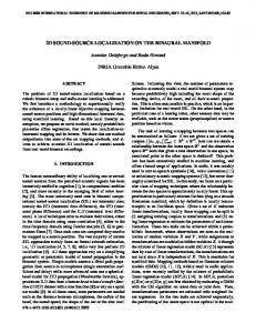
II. MICROPHONE ARRAY MODEL AND SPECTRAL WEIGHTING GCC-PHAT A. Microphone Array Model We construct a model of microphone array in [17]. The following several questions must be considered for designing the microphone array model: (1) The SSL task to be resolved. (2) The cost of equipments. (3) The computational complexity. (4) The shape of platform where microphone array fixed. The SSL system is used for HRI, which will be described in the following sections in detail. For reducing the cost of equipments and computational complexity, the less microphones are, the better. Localizing the azimuth and the horizontal distance of sound source in 3D space needs more than two microphones. On the other hand, the shape of the robot should be considered. As a result, four microphones with a cross-shaped plane are used. The microphone array is installed on a horizontal plane of the robot with a specific height. For the purpose of horizontal distance localization, the aperture of microphone array should be suitable. The topology of microphones array is shown in Fig. 1 .
Fig. 2: The waveform and spectrogram of noise GCC-PHAT method has been widely used to estimate the time delay of two signals collected by different microphones generated by the same sound source. The variable x(t) denotes the signal received by microphone. GCC-PHAT is given in [10] as the following equation: RGCC (τ ) =
∫ ∞ ΦXm Xn (ω )e jωτ −∞
|ΦXm Xn (ω )|
dω
(1)
where X represents the Fourier Transform of signal x, and ΦXm Xn (ω ) is the cross-power spectrum of two signals. Based on the characteristics of noise described above. A spectral weighting function will be proposed. Firstly, the power spectrum of noise can be estimated from forepart of signal: 1 M EV (ω ) = (2) ∑ |Vm (ω )|2 M m=1 where Vm (ω ) denotes the spectrum of the mth noise frame and M represents the number of noise frame. In addition, the power of the current noisy signal frame is EX (ω ) = |X(ω )|2 . The posterior SNR value of frequency ω is:
γ (ω ) = max(
EX (ω ) , 1) EV (ω )
(3)
For two signals xm (t) and xn (t), the posterior SNR γm (ω ) and γn (ω ) can be obtained. Then the spectral weighting function is proposed as: Ψ(ω ) = min{(logκ γm (ω ))β , (logκ γn (ω ))β } Fig. 1: Microphone array model B. Spectral Weighting GCC-PHAT The waveform and spectrogram of noise when a mobile robot works in real environment are shown in Fig. 2. It is obvious that noise is generated by several specific noise sources, such as motor of the robot, air conditioning and computer fans. Therefore, it will be spatial correlated. In
(4)
where κ can be adjusted in different environments to keep the weight reasonable, the greater overall SNR value is, the greater κ should be. And β is also adjustable, which controls the divergence of weighting coefficient, the greater β is, the greater divergence will be. This two parameters should be determined empirically based on experimental environments and the performance of the SSL system. In addition, the aperture of microphone array is not small enough, so different signals collected by different microphones will be affected
2880
2) The relationship between τd and |si − sj |: { |αi − α j |, for |αi − α j | < 180◦ (9) τd ∝ 360 − |αi − α j |, for |αi − α j | ≥ 180◦ { |di − d j |, for di < d j τd ∝ (10) di − d j , for di ≥ d j { |hi − h j |, for 0 < hi < h j τd ∝ (11) hi − h j , for hi ≥ h j > 0
by noise with varying degrees. Selecting the smaller value as the weight is essential to guarantee that both of signals should be affected by noise weakly which has big weight. Finally, the SW-GCC-PHAT function can be written as: RGCC (τ ) =
∫ ∞ −∞
Ψ(ω )
ΦXm Xn (ω )e jωτ dω |ΦXm Xn (ω )|
(5)
III. SPATIAL DISTRIBUTION OF TIME DIFFERENCE FEATURE AND GRID MATCHING
This property reveals the positive relationship between the difference of feature vectors and the difference of azimuth, horizontal distance and height respectively. Which concludes that the farther the distance between two sound sources is, the greater the difference between two feature vectors becomes. This relationship is shown in Fig. 3, where αi , di and hi is selected randomly, and they are representative.
In this section, the time difference feature of sound source and its spatial distribution are presented in Part A. Then, a novel localization method based on the spatial property of time difference feature, termed Space Grid Matching (SGM), is proposed in Part B. A. Spatial Distribution of Time Difference Feature The symbol τmn denotes time difference of two signals recorded by m-microphone and n-microphone. The number of microphone used in the SSL system is M. Then M(M − 1)/2 pairs of time difference can be obtained, and only M −1 pairs of them are independent mutually. However, the measurement of time difference always exists deviation, even mistake. And more time differences are, more robust. Therefore, all time differences are combined into feature vector as: (6)
The coordinate of sound source Si and microphone Rm are defined as si = [xsi , ysi , zsi ] = [di cos(αi ), di sin(αi ), hi ] and rm = [xrm , yrm , zrm ], where αi , di and hi are the azimuth, horizontal distance and height of sound source Si . Then, the feature vector of sound source Si can be computed as: dSi Rm = ∥si − rm ∥ dSi Rn = ∥si − rn ∥
τSi Rmn = (dSi Rm − dSi Rm )/c τSi = [τSi R12 , τSi R13 , · · · , τSi Rmn , · · · , τSi R(M−1)M ]
(7)
where dSi Rm denotes the distance between Si and Rm and c is the speed of sound. The difference of feature vector between sound source Si and S j is:
τd = ∥τSi − τSj ∥
(8)
where Euclidean distance is used. Considering the microphones array mentioned in section II. The following properties of τd can be obtained. 1) If τd = 0 i.e. τSi = τSj , then αi = α j , di = d j and hi = h j or −h j . Which means a specific time difference feature vector corresponds to two sound sources that are symmetric with respect to the plane of microphone array. But the negative h j is neglected in the application of HRI. Therefore, the relationship between feature vector and sound source is one-to-one correspondence.
Height Azimuth Horizontal distance
6
The difference between τi and τj
τ = [τ12 , τ13 , · · · , τmn , · · · , τ(M−1)M ]
−4
x 10
5
4
3
2
1
0
0
di
αi
hi
The variety of αj, dj and hj
Fig. 3: The relationship between τSi andτSj B. Space Grid Matching (SGM) Localization Algorithm As mentioned in Part A, one sound source corresponds to one time difference feature vector, vice versa. Moreover, two adjacent sound sources produce a pair of similar feature vector. The horizontal plane can be divided into many grids with a certain size. The partition of horizontal space is shown in Fig. 4. Those sound sources in a same grid are adjacent, whose feature vectors are similar. On the contrary, the distance between two different grids is farther, which generates very different feature vectors. Constructing a Gaussian Mixture Model (GMM) as template for each grid based on time difference feature vector using Monte Carlo method. For example, the height of microphone array plane is 1m. For an arbitrary grid, its azimuth distributes from α1 to α2 , its horizontal distance distributes from d1 to d2 . The GMM of this grid can be trained offline as: 1) Initializing a Gaussian Mixture Model. 2) Generating a azimuth α randomly, α ∼ U(α1 , α2 ). 3) Generating a horizontal distance d randomly, d ∼ U(d1 , d2 ).
2881
(a) Horizontal distance
(b) Height
(c) Azimuth
Fig. 5: The spatial distribution of feature difference for horizontal distance, height and azimuth
Fig. 4: The partition of horizontal space 4) Generating a height of male hm randomly, hm ∼ N(0.55, 0.06). 5) Generating a height of female h f randomly, h f ∼ N(0.45, 0.06). 6) Generating a value of gender randomly, then the height h can be selected from hm and h f . 7) The coordinate of this random sound source is [xs , ys , zs ] = [dcos(α ), dsin(α ), h]. The time difference feature vector τ can be computed using Equation 7. 8) Executing N times from step 2 to 7. 9) Training the GMM using these N τ . For localization, the problem to be solved is which grid dose the sound source distribute in, with time difference τ is given. Symbol G denotes a grid. The problem can be described as: Gs = arg max P(G|τ ) G
P(τ |G)P(G) G P(τ ) ∝ arg max P(τ |G)
= arg max
(12)
G
where Gs represents the grid of sound source . This equation means that resolution is the grid which has the greatest likelihood value. All of the likelihood values between each GMM and the current time difference feature vector should
be computed, then the greatest presents the sound source grid. How to determine the size of a grid? Obviously, there is not a upper bound for the size of a grid. Theoretically, any size is correct. However, measurement error of time difference is inevitable. The feature vector difference of two opposite boundary of a grid indicates the sensitivity of this grid to measurement error, more smaller the difference is, more sensitive. The minimize size of this grid is depended on the level of average measurement error and the sensitivity. If the size is smaller than the valid minimize size, the localization result will deviate from real value. Therefore, the feature vector difference of two opposite boundary should be greater than the average measurement error. In particular, the sensitivity is different between each dimension, furthermore, between different areas of one dimension. For example, considering the microphone model mentioned in Section II, and the microphone array plane has a height of of 1m, the distance between two adjacent microphones is set to 0.4m. The average measurement error is set to 0.8 × 10⁻⁴ empirically. Fig. 5 shows the feature vector difference of two opposite boundary of a grid with a specific azimuth, horizontal distance and height size respectively. Obviously, it is isotropic in azimuth dimension, so a arbitrary azimuth is representative. Fig. 5(a) shows the feature vector difference in the whole horizontal distance and height space with a horizontal distance size ∆d = 0.6m. Azimuth is a arbitrary constant, such as α = 30◦ here. In each area, the plane with feature difference 0.8 × 10⁻⁴ can judge whether it is reasonable that the size of horizontal distance is set to ∆d = 0.6m or not. The size of horizontal distance of those areas below the plane can not be equal to or less than 0.6m. Fig. 5(b) shows the feature vector difference with a height size ∆h = 0.1m. Fig.5(c) shows the feature vector difference with a azimuth size ∆α = 2◦ . Similarly, The size of height and azimuth of those areas below the plane can not be equal to or less than 0.1m and 2◦ . It can be seen that horizontal distance and height are more sensitive in far horizontal distance area, azimuth is more sensitive in near horizontal distance area, and the variety of sensitivity is small
2882
between different heights. A reasonable size of a grid in each area can be determined by many feature vector difference figure with different size of each dimension. For example, considering horizontal distance, the feature difference with different horizontal distance size is shown in Fig. 6. Azimuth and height are set to 30◦ and 0.5m. In addition, the task of HRI is also considered. The azimuth should be localized as accurately as possible. The dangerous area and save area of the robot should be distinguished well. Considering the aperture of microphone array, the boundary between far field and near field is in the region of 1.5∼2.5m. We are not interested in the height of sound source. In summary, the minimize size of azimuth is set to 1◦ . The horizontal distance is divided into three parts: NEAR 0∼1.5m, MEDIUM 1∼2m and FAR 1.5∼4m, which correspond to dangerous distance, medium distance and far distance between human and robot. The whole height space is treated as one part.
Decision Tree is used. The number of likelihood value computing becomes 2+2+2+3+3+5+3=20. Firstly, a GMM should be trained for each node of the tree offline, which is high time-consuming. For those nodes of the first seven layers, the horizontal distance is treated as one part. In the 8th layer, the azimuth grope is 1 degree. In the stage of localization, the likelihood value is computed layer by layer from the root of the tree to leaf, just like the trajectory of red line in Fig. 7. In each layer, all children of the current node are matched with τ , then the sound source is located to the sub-grid whose likelihood value is the greatest.
−4
7
x 10
∆d=0.3m ∆d=0.6m ∆d=0.9m ∆d=1.2m
feature difference
6
5
4
3
2
Fig. 7: Decision tree for SGM method
1 0.8 0 0.5
1
1.5
2
2.5
3
3.5
B. Valid Feature Detection (VFD)
4
Horizontal distance
Fig. 6: The feature difference of horizontal distance with different size As we know, geometric positioning method solves localization problem inversely, from time difference to location. The solution of inverse problem has many problems such as nonlinear and high computational complexity. In comparison, SGM method avoids the solution of inverse problem. In addition, it weakens those dimensions that we are not interested in, such as the height dimension. Which is equivalent to reducing the dimension to be resolved. Furthermore, it doesn’t need the assumption of far field or near field. This method is more powerful and efficient than geometric positioning method in some way. IV. DECISION TREE AND VALID FEATURE DETECTION
The wrong time difference will deteriorate the accuracy of localization. Therefore, it is important to remove those invalid features which are wrong. Furthermore, in the application of HRI in noisy environment, if a wrong localization takes place, it is reasonable that the speaker calls the robot again. Valid feature can be detected from one sound or multiple sounds generated at the same position. Here τimn denotes the time difference of the ith sound between m−microphone and n−microphone. Theoretically, the following equation is established:
τimn = τ jmk + τ jkn τimn = τ jmn
k ∈ [1, M], j ∈ [1, I] j ∈ [1, I]
(13) (14)
where M denotes the number of microphones and j denotes the number of sound. Set Γimn is defined as: ei jmnk = |τ jmk + τ jkn − τimn | k ∈ [1, M], j ∈ [1, I]
A. Decision Tree for SGM The computational complexity would be very high if too many grids are divided, since all grids are matched with the current feature vector. For example, it is supposed that the azimuth is divided into 360 parts, the horizontal distance is divided into three parts. There are 360×3=1080 likelihood values should be computed. By contrast, as shown in Fig.7,
ei jmn = |τimn − τ jmn |
j ∈ [1, I]
Γimn = (ei jmnk |ei jmnk > th) ∪ (ei jmn |ei jmn > th)
(15)
where th is a threshold, if ei jmnk is greater than th, the equation (13) for τimn , k and j is discrepancy. Similarly, if ei jmn is greater than th, the equation (14) for τimn , j is
2883
discrepancy. The element number of set Γimn is qimn . Then, the validity of τimn can be defined as: { valid, for qimn < T H τimn is (16) invalid, for qimn ≥ T H. where T H is a threshold decided by the number of microphone M and the number of sound I. If the number of unmatched pairs defined by (15) is greater than T H, the time difference τimn is considered to be invalid. Finally, computing the mean value of the valid feature of multiple sounds, these features correspond to the same microphone pair: ′
τmn =
1 ∑ τimn J valid τimn
on the shoulder of the robot with a height of 1m, and the distance between two adjacent microphones is 0.4m. Four BSWA MPA416 microphones and a MARIAN TRACE8 multi-channel audio sample card are used for the sampling of sound. The sampling rate is 44.1kHz. The scene of experimental environments, robot and microphones is shown in Fig. 9.
(17)
where J presents the number of valid τimn . If J = 0, τmn is ′ invalid and it will be removed. All valid τmn are combined ′ into a new feature vector τ . Overall, the flowchart of SSL algorithm mentioned above is shown in Fig. 8. VFD method uses one time difference vector τ1 or multiple vectors τ1 , · · · , τm . The GMM library is trained offline, which includes all templates corresponding to every node of Decision Tree.
Fig. 9: Scene graph of a robot and microphone array
B. Sound Source Localization on Stationary Robot
Fig. 8: The flowchart of SSL algorithm V. EXPERIMENTS AND ANALYSIS In this section, experiments of SSL for HRI are implemented. Configuration of experimental environments is described in Part A. Part B gives the Localization results and analysis of stationary robot. Experiments for HRI is presented in Part C. A. Configuration of Experimental Environments The mobile robot works in a hall, semi-door environment, with a size of 8m×8m. The microphones model is described in Section II, the microphones array is placed
In this experiment, the stationary robot is placed in the center of the hall, the sound source to be localized is placed on another 96 positions in the vicinity of microphones array, with the azimuth of every 15 degree and the distance of 1, 2, 3, 4m from the center. The greater the distance between the sound source and the microphone array is, the greater noise would be, the lower overall SNR is. If the horizontal distance of sound source is no more than 3m, the overall SNR is 15dB, whereas, the overall SNR is 10dB. In each position, 21 groups of speech data from different people are recorded, the content of speech is Chinese word ”dingwei”, ”pengpeng” and ”guolai” which mean ”location”, ”Robot’s name” and ”come here” respectively. Therefore, in total of 96×21=2016 sets of data are tested. The localization accuracy of azimuth is 1◦ , and the azimuth localization correct rate has 4 kinds of situations, the difference between localization result and real value is less than 5◦ , 10◦ , 15◦ and 20◦ respectively. The horizontal distance is divided into three parts: NEAR 0∼1.5m, MEDIUM 1∼2m and FAR 1.5∼4m. The whole height space is treated as one part. The number of component of GMM affects the localization performance. Its value is determined by the scale of grids. The azimuth localization performance with different mixture number is shown in Table I. In this experiment, the basic SGM method is used, and those data with horizontal distance of 1, 2, 3m are tested. Obviously, the best performance is obtained with 4 mixtures. Therefore, the number of mixture of GMM is set to 4. The analysis of noise and SW-PHAT-GCC method were proposed in Section III to reduce the influence of noise,
2884
TABLE I: The Selection of Mixture Number GMM MixNum 1 2 4 6 8
TABLE III: Azimuth Localization Using VFD method
Azimuth Correct Rate(%) 5◦ 10◦ 15◦ 20◦ 94.64 97.22 98.61 98.88 94.44 97.09 98.61 98.88 95.17 97.42 98.68 99.01 94.58 97.22 98.61 98.88 94.97 97.09 98.61 98.88
Experimental Condition 1∼3m 1 sound (15dB) 1 sound 4m (10dB)
2 3 4 5
TABLE II: Azimuth Localization Using SW-GCC-PHAT method
sounds sounds sounds sounds
— VFD — VFD VFD VFD VFD VFD
Azimuth Correct Rate(%) 5◦ 10◦ 15◦ 20◦ 97.55 98.81 99.07 99.14 98.35 99.60 99.67 99.67 83.13 85.52 86.71 87.70 93.45 94.05 94.64 94.84 95.73 96.88 97.36 97.36 96.77 97.54 97.82 97.82 97.90 98.49 98.57 98.59 98.49 99.01 99.05 99.15
TABLE IV: Horizontal Distance Localization Experimental Condition 1∼3m GCC-PHAT (15dB) SW-GCC-PHAT 4m GCC-PHAT (10dB) SW-GCC-PHAT
Azimuth Correct Rate(%) 5◦ 10◦ 15◦ 20◦ 95.17 97.42 98.68 99.01 97.55 98.81 99.07 99.14 73.21 77.98 82.14 82.34 83.13 85.52 86.71 87.70
1
which is narrow band and spatial related. The greater SNR of a frequency band is, the greater weight this frequency band will have. The azimuth localization results of this method are shown in Table II. Where the parameter κ and β are set to 10 and 0.55 empirically. Then, the spectral weighting function can be written as Ψ (ω ) = min{(log10 γm (ω ))0.55 , (log10 γn (ω ))0.55 }. Two kinds of experimental situations with different overall SNR are tested. Comparing the performance of SW-PHAT-GCC method with PHAT-GCC method, Spectral Weighting improves the correct rate largely. In particular, it is more effective in low SNR situation. Decision Tree reduces the matching times between the GMM of each grid and the TDOA feature dramatically. As mentioned in Section IV, the matching times are reduced from 1080 to 20 for each localization, and the matching stage takes 40 milliseconds reduced from 640 milliseconds in our experiments. The azimuth localization results using VFD method are shown in Table III. In the high SNR area, one sound is adequate. However, in high SNR environment, the performance deteriorates dramatically. More than one sounds generated at the same position are necessary. The more sounds are, the better the performance will be. However, too many sounds are not available in the application of HRI, generally, no more than three sounds are used. In these experiments, Spectral Weighting and Decision Tree are used. The number of microphone is M = 4, the number of sound is I, so the parameter th and T H mentioned in Section IV are set to 0.23ms and M × I/2 empirically. The horizontal distance localization results are shown in Table IV. It can be seen that more than 90% correct localization rate is obtained. It can judge whether the sound source is standing in the dangerous area effectively. Moreover, our method can handle the problem of the switch between far field and near field easily, which is difficult for geometric positioning method. In other words, SGM method doesn’t need the assumption of far field or near field.
2 3 4 5
No. of Sound GCC-PHAT SW-GCC-PHAT VFD VFD VFD VFD VFD
Horizontal Distance(%) 1∼3m 4m 87.30 73.25 88.82 75.00 90.08 87.70 92.32 89.74 93.40 90.95 94.03 92.06 94.20 92.72
In addition, the experiment using a part of time difference features from a microphone sub-array with three microphones is also implemented. The problem of SSL is unsolvable in 3D space for geometric positioning method using three microphones, because only two independent time difference values can be obtained. SGM method can weaken those dimensions that we are not interested in, such as the height dimension. Which makes it is possible that solving high dimension problem with a small amount of microphones. The localization results using only those features of three microphones in the higher SNR environment are shown in Table V, where ”123” denotes the sub-array that contains the 1th, 2th and 3th microphone, the same to others. ”Mean” denotes the mean value. In this experiment, SW-GCC-PHAT, SGM, Decision Tree and VFD are used. However, it can be seen that the performance is lower than four microphones. C. Experiments for Human-Robot Interaction In the scene of HRI, human call the mobile robot to attract its attention, then the auditory system of the robot collects speech signals and gives feedback to the speaker. Auditory system consists of automatic speech recognition sub-system and sound source localization sub-system. In this experiment, the mobile robot works in the hall mentioned above with
2885
TABLE V: Localization Results Using Sub-Feature SubFeature 123 234 341 412 Mean
5◦ 89.95 90.74 97.55 98.08 94.08
Azimuth (%) 10◦ 15◦ 99.14 99.27 98.88 99.21 98.28 99.14 98.81 99.07 98.78 99.17
20◦ 99.34 99.27 99.14 99.14 99.22
Horizontal Distance(%) 80.49 81.55 86.64 84.26 83.24
3 ∼ 5 people around it. Speech commands includes Chinese word ”pengpeng” and ”guolai” which mean ”Robot’s name” and ”come here”. Firstly, human call the robot, the meaning of the command and the position of sound source can be obtained. Then the robot turns to the speaker, and the vision system is also used to detection the direction of human accurately, such as ”Human Detection” and ”HandsRaising Detection”. In addition, if the horizontal distance is localized as NEAR which means that the speaker stands in the dangerous area, the robot calls attention to him that ”Pay attention, you are standing in the dangerous area”. Secondly, if the command is ”pengpeng”, the robot stays put. Whereas, if ”guolai” is called and the horizontal distance is FAR, then the robot moves 1m toward the speaker. In this step, human can call ”guolai” several times to get a appropriate distance between human and robot. Finally, the robot faces to the speaker directly with a suitable distance. Which is prepared for another interaction tasks. Sound source localization system can localize the azimuth and judge whether the speaker stands in the dangerous area effectively. Experiments for HRI is shown in Fig. 10.
Fig. 10: Experiments for Human-Robot Interaction
VI. CONCLUSIONS In this paper, a novel sound source localization method for mobile robot based on the time difference feature and space grid matching (SGM) method is proposed. SW-GCC-PHAT method estimates the time difference in noise environment, which handles narrow band and spatial related noise well. Time difference feature of a sound source is constructed, and its spatial distribution properties are analyzed. Based on the properties of the distribution, space grid matching method is proposed for localization step. Firstly, it avoids the difficulty of the resolution of inverse problem, which makes geometric positioning method difficult in some situation. Then, it can handle the problem of the switch between far field and near field easily. In addition, it can weaken some dimensions selectively, which reduces the valid dimension. Therefore, it can solve some questions that geometric positioning method can not. Decision Tree reduces the matching times and computational complexity dramatically. VFD removes those wrong time difference features and improves localization per-
formance. Several experiments are presented, which proves the effectiveness of these algorithm. VII. ACKNOWLEDGMENTS This work is supported by National Natural Science Foundation of China(NSFC, No.60875050, 60675025), National High Technology Research and Development Program of China(863 Program, No.2006AA04Z247), Shenzhen Scientific and Technological Plan and Basic Research program (No.JC200903160369A), Natural Science Foundation of Guangdong(No.9151806001000025). R EFERENCES [1] I.E. Robert, ”Robust sound localization: An application of an auditory perception system for a humanoid robot”, MIT Department of Electrical Engineering and Computer Science, 1995. [2] Q.H. Wang, T. Ivanov and P. Aarabi, ”Acoustic robot navigation using distributed microphone arrays”, Information Fusion, 2004, pp. 131140. [3] J. Hornstein, F. Lacerda, M. Lopes and J. Santos-Victor, ”Sound localization for humanoid robots - building audio-motor maps based on the HRTF”, in IEEE International Conference on Intelligent Robots and Systems, Beijing, China, 2006, pp.1170-1176. [4] K. Nakadai, H. G. Okuno, H. Nakajima, Y. Hasegawa and H. Tsujino, ”An Open Source Software System For Robot Audition HARK and Its Evaluation”, in IEEE-RAS International Conference on Humanoid Robots, Daejeon, Korea, 2008, pp. 561-566. [5] C.T. Ishi, O. Chatot, H. Ishiguro, N. Hagita, ”Evaluation of a MUSICbased Real-time Sound Localization of Multiple Sound Sources in Real Noisy Environments”, in IEEE International Conference on Intelligent Robots and Systems, St.Louis, USA, 2009, pp. 2027-2032. [6] H. Wang, M. Kaveh, ”Coherent signal subspace processing for the detection and estimation of angles of arrival of mutiple wide-band sources”, in IEEE Transactions on Acoustics, Speech and Signal Processing, vol.33(4), 1985, pp. 823-831. [7] M. Wax, T. Kailath, ”Optimum localization of multiple sources by passive arrays”, in IEEE Transactions on Acoustics, Speech and Signal Processing, vol.31(5), 1983, pp. 1210-1217. [8] G. Carter, ”Variance bounds for passively locating an acoustic source with a sysmmetric line array”, Journal of Acoustical Society of America, vol.62(4), 1977, pp. 922-926. [9] G.C. Cater, ”Special Issue on Time Delay Estimation”, in IEEE Transactions on Acoustic, Speech and Signal Processing, vol.49(1), 1981, pp. 12. [10] C.H. Knapp, G.C. Carter, ”The generalized correlation method for estimation of time delay”, in IEEE Transactions on Acoustics, Speech and Signal Processing, 1976, pp. 320-327. [11] B. Champagne and A. Stephene, ”A new cepstral prefiltering technique for estimating time delay under reverberant conditions”, Signal Processing, vol.59(3), 1997, pp. 253-266. [12] J. Benesty, ”Adaptive eigenvalue decomposition algorithm for passive acoustic source local- ization”, Journal of Acoustical Society of America, vol.107(1), 2000, pp. 384-391. [13] S. Doclo and M. Moonen, ”Robust time-delay estimation in highly adverse acoustic environ- ments”, in Proceedings of IEEE Workshop on Applications of Signal Processing to Audio and Acoustics, New Paltz, NY, 2001, pp. 59-62. [14] T.G. Dvorkind and S. Gannot, ”Time difference of arrival estimation of speech source in a noisy and reverberant environment”, Signal Processing, vol.85(1), 2005, pp. 177-204. [15] W.H. Foy, ”Position-localization solution by Taylor-series estimation”, IEEE Transactions on Aerospace and Electronic Systems, vol.12(2), 1976, pp. 187-194. [16] JM. Valin, F. Michaud, J. Rouat and D. Ltourneau, ”Robust Sound Source Localization Using a Microphone Array on a Mobile Robot”, IEEE/RSJ International Conference on Intelligent Robots and Systems, Las Vegas, Nevada, 2003, pp. 1228-1233. [17] H. Liu and M. Shen, ”Continuous Sound Source Localization based on Microphone Array for Mobile Robots”, IEEE/RSJ International Conference on Intelligent Robots and Systems, Taipei, Taiwan, 2010, pp.4332-4339.
2886