Space-Time Kernel Density Estimation for Real-Time Interactive Visual ...

Proceedings of the 50th Hawaii International Conference on System Sciences | 2017

Space-Time Kernel Density Estimation for Real-Time Interactive Visual Analytics Todd Eaglin UNC Charlotte [email protected]

Isaac Cho UNC Charlotte [email protected]

Abstract We present a GPU-based implementation of the Space-Time Kernel Density Estimation (STKDE) that provides massive speed up in analyzing spatialtemporal data. In our work we are able to achieve subsecond performance for data sizes transferable over the Internet in realistic time. We have integrated this into web-based visual interactive analytics tools for analyzing spatial-temporal data. The resulting integrated visual analytics (VA) system permits new analyses of spatial-temporal data from a variety of sources. Novel, interlinked interface elements permit efficient, meaningful analyses.

William Ribarsky UNC Charlotte [email protected]

accelerate the KDE. As part of their work they reviewed all prior KDE techniques and benchmarked performance. Through their work they have produced the fastest known implementation for a 3D KDE, but even that implementation is not fast enough for producing a sub-second, real-time approach. But if an interactive STKDE could be developed, it would be a boon for analyzing clusters and hotspots in time. The effects of latency on exploratory VA can be significant. Liu et al. [20] showed that even a 500ms

1. Introduction The amount of space-time data has exploded in recent years due to new technologies [19]. It can be extremely difficult and computationally challenging to analyze, visualize and extract meaning from spatiotemporal data in a real-time application. There is a need to find clusters and hotspots in space-time in order to drive further analysis [5]. Using a Kernel Density Estimation as part of an interactive tool is an effective way to analyze geospatial hotspots [23] [22]. Since these density estimations are usually 2D and are typically applied to spatial extent, important temporal behavior or combined space-time behavior can remain hidden. Using a space-time kernel density estimation, it is possible to find clusters to reveal this behavior, but there are critical limitations. Delmelle et al. [4] explored the use of the space-time kernel density estimation on dengue fever outbreak in Cali, Columbia. This work demonstrated the computation challenge, but also the potential payoff, of the STKDE. Recently, there have been several prior works that focus on speeding up the KDE. Hohl et al. [14] have used a parallel CPU approach to compute the STKDE. In their method they use a spatial decomposition initially to subdivide the work load among a defined set of CPUs. Michailidis et al. [24] focused on using the GPU to accelerate the KDE using memory sharing techniques. The most recent work in this area by LopezNovoa et al. [21] used crop and chop techniques to

URI: http://hdl.handle.net/10125/41318 ISBN: 978-0-9981331-0-2 CC-BY-NC-ND

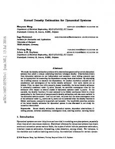
Figure 1. Overview of our web-based tool. (A) Temporal View with selection made. (B) 3D view with STKDE structure and slicing planes. (C) 2D spatial view for temporal slice. (D) Spatial Slice.

delay had a dramatic impact on user’s actions. It limited the ability of users to generate effective decisions from analytical tools. Therefore, minimizing latency in VA is one of major constraints for incorporating the STKDE into an interactive VA tool. GPU computing has advanced significantly in re-

1381

cent years to accelerate specific types of computationally intensive tasks [26]. In addition, GIS tasks can substantially be improved through parallel processing [31]. In this work we develop a GPU-based algorithm for accelerating STKDE for real-time analysis. Our focus is to optimize the STKDE for results that will be sent over the Internet. As the voxel count grows so does the transfer of data from the server. We thus are not as focused on larger voxel counts for the STKDE computation because it would be unrealistic to send the resulting calculations over the Internet in real time. Kapler et al. developed GeoTime for visualizing trends in space-time [15]. But, our focus is more on identifying hotspots and not trends over time. Kaya et al. [16] explored the usage of 3D and 2D on spatiotemporal data. In their evaluations, they examined the benefits and disadvantages of using 2D and 3D. For their visualizations they used heat maps for 2D and stacked heatmaps for 3D. They concluded that neither 2D nor 3D is significantly better for analyzing spatiotemporal data. But the use of stacked heatmaps in 3D does not take into account the relationship between different points in time, as does our approach. It just uses slices at different time intervals stacked together. In addition, it may be that the data to which they applied their analyses does not show the distinct spacetime structure that we see in our 3D STKDE analysis. Nakaya et al. [25] explored the use of STKDE on visualizing crime clusters. Klemm et al. [17] explored the use of 3D heatmap visualization for population data. They found that the 3D visualization worked very well as an overview of the entire data. Clusters or areas of interest could be spotted quickly and from that point additional exploratory analysis could be pursued. Brundson et al [1] explored the use of STKDE in visualizing crime patterns in space and time. Demsˇar et al. [7] studied using STKDE for trajectory data mining. Gao et al. [11] used STKDE to visualize the impact of publications across space and time. In other work Gao et al [10] explored STKDE compared to other spacetime techniques and concluded that STKDE is much easier to visually identify clusters and areas of interest. In this paper we focus on three aspects of the spacetime kernel density estimation. • Scale - Due to the nature and sheer volume of spatiotemporal data, it can be computationally difficult to do any analysis at scale or in real-time. Even small amounts of latency can have dramatic effects on interaction. Therefore, we focus on improving the existing state of the art. • Interaction - Without scale and real-time it is hard to achieve effective interaction. • Visual Analysis. Lastly, we need an easy to use VA approach with multiple coordinated views for visualizing different aspects of the STKDE.

Based on our results, we see the STKDE as an important addition that should be integrated with a larger set of tools for understanding and exploring space-time data. In section 2 we detail our GPU-based algorithm discussing the underlying data structure used and the implementation with initial results. In section 3 we detail how we’ve incorporated our approach into a real-time VA tool with novel interlinked interaction. In section 4 we discuss the results of our work. This includes the performance metrics achieved by using the approach and how it compares to the current state of the art. Gomez et al. [12] examined effective methods for evaluating spatiotemporal VA. We incorporated this methodology into our evaluation. We include a small user evaluation using our approach in an interactive VA tool. We also cover several use-cases of our technique.

2. Algorithm In this section, we detail our strategy for operating on each voxel independently in order to fully utilize parallel processing. For each voxel in a 3D region the density is calculated based on surrounding data points that fall within a spatial and temporal bandwidth, which are then weighted using an Epanechnikov kernel function as indicated in the equation below. For each voxel given the coordinates (x,y,t) the density is estimated based on the surrounding data points given as (xi, yi, ti). The spatial and temporal distances between the voxel and data point is given by di and ti. The spatial and temporal bandwidths are given by hs and ht.

2.1. Oct-Tree/GPU data structures During our work on LiDAR analysis, we incorporated GPU-based techniques for analyzing massive LiDAR datasets [8]. In that work we used a Quad-Tree with pruning and spatial indexing [13] to optimize data lookup on the GPU. These techniques were a starting point in optimizing our workflow for doing the STKDE. On the GPU we are limited in several ways. There are memory limitations, hardware limitations, and limitations in the programming API itself. This meant we had to work around not having a deep call stack, no recursion, no pointers, limited local memory, and thread divergence. Therefore, we had to use an optimized data structure. We store the Oct-Tree as a pre-order indexed array. To reduce the memory footprint and lookup complexity we prune the tree depth based on the GPU memory limit. This limit is defined by the max buffer size specified by the OpenCL driver. We then use that size to calculate how many data points we can store in a single cell. We take each leaf node to create a cell with an

1382

index for each point inside that leaf node. We store the cells in first-in order in an indexed array. The indices of the cells are used to create a cell range lookup. During the building process the cell ranges are stored at each node in the tree. After constructing the tree we then thread the tree. The purpose of threading the tree is that on the GPU we cannot use recursion nor is using a stack type data structure feasible. Since our tree is stored in a pre-order fashion we can iteratively step through the top level nodes of the tree quickly isolating sections that fit within the space-time bandwidth. As the algorithm steps through the tree it needs to know where to go next if a particular node does not fit within the space-time bandwidth or it does not contain any more children. This is the purpose of the thread. It is an index for the next location into the array of nodes. In prior work by Wang et al. [33], a decomposition step was performed to optimize the work load between processors using a quad tree for grid computing. Our parallel algorithm diverges significantly at this point. We bypass doing a decomposition step as it is not necessary using our data structure, and we operate at the voxel level. This is done by creating a threedimensional global work group using the voxel dimensions.

guage like Python. We implemented everything not related to the OpenCL computation into C++. This gave us the control we needed for managing memory and data structures. We then wrapped all of it into a Python binding. This allowed us to calculate the STKDE from a high level language, but retain all the control and performance from C++. For the OpenCL computation we only use one kernel function. This function operates on each voxel in the space-time bounds. In our implementation we automatically detect an optimal voxel size unless one is strictly given. We used the approach detailed in [29] to compute an optimal bandwidth spatially and temporally. As a result of these efforts, we were able to achieve great performance. We used a Dengue Fever dataset [14]. We initially tested two different configurations: one using just the CPU and one using just the GPU. We used the same dataset and increased the voxel

2.2. Implementation

Figure 2. Axis-aligned (A) and non-aligned (B and C) spatial slicing results. The image returned contains the contours of the slice and the aggregation across space and time. The time units are in days and the spatial units are in meters with respect to the map projection used.

We implemented our technique using OpenCL; in this way we could evaluate the performance of running either on the GPU and CPU. In order to make our approach more accessible and easy to use we incorporated it into a high level lan-

count for each run. As the starting benchmark, we were able to process 6.3 million voxels in 0.636 seconds on the GPU, and 3.425 seconds on the CPU. We also incorporated one more optimization that can be used for larger data sets. Instead of computing the influence of each sample point in a given leaf node we

1383

can use the centroid of those points for a given leaf. The points in the leaf are very similar to each other and using the centroid is a slight approximation that can have a significant performance boost. During the construction of the tree we compute and save the centroid for each leaf. We then compute the density given this one point weighted based on the number of points in the leaf. As the data points grow this technique becomes more effective. For example, given an average of 10 points per leaf node this can effectively reduce the data size by a factor of 10. We ran this technique on the Dengue Fever dataset. We were able to now process the same 6.3 million voxels on the GPU in 0.387 seconds and 1.22 seconds on the CPU. In algorithm 1 we provide pseudocode for the non-coalescing version of the algorithm. The variables hs ht are the spatial and temporal bandwidths. voxelSize is the dimensions of a single voxel. bbMin is the minimum point on the bounding box that contains all voxels. Lastly, globalId is a built in OpenCL call for getting the global position of a thread with respect to the global work group. The centroid version of this algorithm removes the inner for loop and uses a center point instead of acquiring a data point.

3. Visual Analytics In this section, we discuss how we created an integrated VA tool for visualizing and interacting with the STKDE. We utilized multiple coordinated views following the guidelines in [27]. We set up our technique as a web-service using a GPU computing server.

3.1. Web Based Design One of our major goals with this work was to make it accessible, plugin free and easy to use right from a web-browser. A web-based tool could be easily accessed and used with minimal hardware and software. Delmelle et al. [6] developed a web-based tool for visualizing Dengue Fever. Cho et al. [2] developed a webbased analytical system for visualizing temporal and spatial data in multi-coordinated views. We followed their paradigm using WebGL, an OpenGL ES version for web browsers, and establishing the STKDE computation and visualization as a webservice. As we detail in the implementation section, we developed this approach with the goal of incorporating it into a high level language like Python. We calculate the STKDE in a Python framework (permitting easy integration with existing frameworks and data analytics tools) and embedded it into a web service on a GPU server. In order to visualize the STKDE, we needed a 3D mapping system that could be integrated with existing web-based tools and multi- coordinated views. All of the existing mapping tools like Google Maps, Apple Maps, Bing, etc. did not have extensive 3D capabili-

ties. The mapping tool also needed to have an easy way to incorporate custom 3D geometry. In prior work [9] we developed such a mapping system for mobile devices using OpenGL. Our mapping system was built in 3D, but used a 2D projection. Therefore, we ported it to WebGL using ThreeJS.

3.2. 3D View In this section, we discuss the importance of our 3D view, some of the interactions, and how it is coordinated with other views. The 3D view is the most important view for visualizing our space-time kernel density estimation. We’ve incorporated a 3D tile map with level of detail that you would see in other existing mapping systems. The 3D view has several interactions. The first is rotating. We utilize an orbiting camera fixed around a focal point. A user can rotate the camera around the focal point by dragging with the left mouse. This is typical interaction you would find in a 3D application. The second is panning, using the right mouse a user can pan the 3D view based on the viewing angle with relation to the up vector of the 3D scene. The third navigation interaction is zooming, which can be done using the mouse wheel. Lastly, there is interaction with the 3D structures produced by the space-time kernel density estimation. These interactions include slicing, which is further discussed in the section on slicing. The view is also linked with the other existing views, both the 2D spatial view, and the temporal view. Using a 3D perspective introduces uncertainty and ambiguity into the visualization. Ambiguity can cause significant problems for users trying to use VA systems. Examples of these ambiguities include trying to visually discern where different 3D features exist spatially and temporally in relation to one another. This is crucial for understanding orientation and position of 3D structures without significant cognitive load. The first step we do is utilize a space-time cube around the entire STKDE. The lowest point on the Z axis corresponds to the oldest date and the highest point is the most recent. This technique was used in prior work and proved very effective for helping to discern the bounds both spatially and temporally of given 3D structures. The space-time kernel density estimation does not generate any information about the center of clusters, but additional techniques can be used to find the high density centers. In order to minimize the spatial ambiguity, we use the mean shift algorithm [3] in order to find high density centers. This works by providing the algorithm only voxel centers with a high density. Once we find the high density centers we create a center line to the surface of the 3D map. For rendering we utilize phong shading with specular highlights in order to enhance and visually detail the surfaces. We also apply a slight transparency

1384

to the surfaces to help with occlusion. This can be seen in figure 2.

3.3. Surface Extraction As part of the visualization we use isosurface extraction to approximate the surface for a given density in order to create 3D structures. For the purposes of this work, we do not delve into this area because the field of isosurface extraction has been well researched. While isosurface extraction can have a high time complexity, the topic has been explored deeply with numerous techniques that aim to improve performance. We realized that no matter how long the Space-Time Kernel Density Estimation took if the isosurface extraction took a long time as well it would be detrimental to our work and would hinder using the technique in real-time analytics. Therefore, we opted to using a parallel GPU-based marching cubes to help improve computation time. Our efforts in this area could be further improved by more recent work that could be incorporated into our systems. Smistad et al. [30] developed a real-time technique for surface extraction that uses GPU computing and histogrampyramids to further optimize surface extraction.

3.4. Caching, Compression, and Data Format Caching is one of the most crucial aspects of our web-based design. In prior work [9], a mobile clientserver architecture was developed for hurricane simulation ensemble data. We used the design principles from this work for establishing our caching system, compression process, and the data format. For the data format we stored the data as a compressed JSON of the raw indexed triangles, vertices, and normals.

3.5. Slicing In this section we detail two interactions we incorporated to further explore and analyze the space-time kernel density estimation. Klemm et al. [17] incorporated substantial usage of slicing planes in their work on 3D regression heatmap analysis. For the purposes of our work we incorporate two different types of slicing. Temporal slicing involves selecting a region in time and viewing just that slice in a 2D-spatial view. Spatial slicing involves selecting a region in space and viewing the slice across all time just for that region. 3.5.1. Temporal-Slicing. As part of our tool, we incorporated a coordinated time graph linked with the other views. Walker et al. [32] explored different timeseries visualizations for effective interactions. We found the best choice to be a brush + zoom interaction and visualization. We provide a time graph that depicts the entire time-signature across the entire data set. A user brushes along this global time view to make a selection. Then a zoomed in portion of the time graph for that selection is created to show a more detailed view of temporal events. The time graph selection generates a corresponding bounding box in the 3D view

that specifics the region in time that was selected. In the 2D view we generate a heatmap using just a kernel density estimation. This is all shown in the over view in figure 1. In the user evaluation detailed later we examined our tool with just temporal slicing. After doing the evaluation we realized that additional work had to be done for different types of slicing and that temporal slicing alone was not enough. Thus, from that evaluation we learned that we needed to add spatial slicing due to the unique structures created via the STKDE. 3.5.2. Spatial-Slicing. Spatial slicing is a new technique that arises from the STKDE. It is important because the STKDE volume is often not symmetric around its perpendicular axis. It may be stretched in one direction or have a bump; it may merge with another volume in a particular direction. The temporal behavior of a slice in one direction can thus be significantly different than that in another direction, and this difference can be meaningful, as we will discuss further in the use cases below. Therefore, it is important to quickly and easily set up slicing so that volumetric features can be accessed with reasonable precision and lack of ambiguity. In the same way that temporal slicing shows a distinct region across time, spatial slicing shows a slice in space. We looked at several options for implementing the interaction for spatial slicing. Our goal is to make the tool as straightforward as possible, but there could be situations where the slicing plane needed to be angled away from an axis. Ultimately we opted for doing the slicing in the 3D view. Instead of adding elaborate menu items for changing interaction modes, we used double clicking in the 3D view to select regions on the wireframe bounding box of the space-time kernel density structures. The process works as follows. A user selects a point on the wireframe bounding box. This generates a perpendicular dotted line from the wireframe selected. An example of this can be seen in figure 2A. At the end is a large point that the user can double click to complete the line segment and create the slicing plane. We incorporated this option because it would be difficult for a user to make a perfectly axisaligned slicing plane if he or she wanted to. Otherwise, the user can select any other point on the top of the wireframe to create an angled slicing plane (figures 2B and 2C). This is the minimal amount of effort and bypasses the need for more complex interactions. The resulting slice is shown in figure 2. The contours provide a detail analysis. The user can see how they spread in the selected spatial direction over time and, in this case end abruptly. In addition, the image shows temporal and spatial components aggregated at the right side and stop, respectively. Thus, for example,

1385

the right side shows the timeline along the selected spatial direction. Implementing spatial slicing was more technically challenging than temporal slicing because a lot of the existing tools for doing the data extraction and visualization could not be used for spatial slicing. Additional work also had to be done in order to handle angled slicing planes. Therefore, we had to fully develop a process for generating the spatial slice through our web-services and then visualize. We examined several options, but we ended up doing server-side rendering of the data to an image. Our goal was to keep the client application as thin as possible. Using server-side rendering is very fast because we already have the GPU hardware for doing computation. Due to the caching system in place, acquiring the data on the server-side is a trivial task and requires minimal computation. Once a user makes a slicing plane selection the client sends the points detailing the plane to the server. The original data computed from the space-time kernel density estimation is voxels. The server calculates the normal of the plane. The normal is used to determine which voxel face to aggregate for rendering. In cases where the plane is not axis-aligned a face can be generated from the diagonals of the voxel. The slicing will find the closest angle. Using the angle, the perpendicular distance between each voxel and the plane is computed based on the center point of the voxel. If the distance is less than or equal to the corresponding voxel dimension, then the face is collected and used. GPU

CPU

GPU-C

CPU-C

S-KDE(i7)

S-KDE(Phi)

1 MILLION

100

50

0 10

18

30

60

Figure 3. Graphed results for 1 Million sample points using mvrnorm. S-KDE is the crop and chop KDE algorithm. GPU-C and CPU-C is our algorithm with coalescing.

4. Results In this section we detail all the results of our SpaceTime Kernel Density Estimation and compare them with the state of the art. We also detail our evaluation

and several use case studies we performed using our techniques and tools.

4.1. Performance In this section we discuss in more depth the performance results achieved by using our GPU-based technique. We also included CPU results for comparison. We’ve placed a heavy emphasis on performance because all of our tools, interactions, visual analysis depend on how quickly we can calculate the STKDE. For all tests we used one CPU configuration consisting of an Intel Xeon with 6 cores at 3.5GHz. We also used a GTX 770 for the GPU benchmarks. In the first part of our performance evaluation we examine our techniques against the state of the art [21]. In their work they evaluate a 3D KDE by generating two synthetic datasets with the mvrnorm function from the R framework, which generates multivariate samples with a normal distribution. We use the exact same approach to generate two sets of data with 500,000 samples and 1,000,000 samples each. We then vary the voxel count in relation to their evaluation tests. We also use the same heuristic approach to compute a bandwidth for the given datasets [29]. For 500,000 samples at 10 million voxels we were able to calculate it in 1.596 seconds on the CPU and 0.937 on the GPU. Using coalescing we were able to improve the time further to 0.74 seconds on the CPU and 0.679 on the GPU. For 1 million samples at 10 million voxels we were able to calculate it in 2.17 seconds on the CPU and 1.184 on the GPU. Using coalescing we were to achieve 0.9 seconds on the CPU and 0.727 seconds on the GPU. Compared to previous work we were able to achieve over 10 times an increase in performance as shown in figure 3. We acquired a copy of the Dengue Fever data from prior work to evaluate our algorithm [14]. For our comparisons we used the same data, the same temporal, spatial and voxel size in order to maintain control on all these metrics. The data consisted of roughly 7,000 space-time points and the voxel count used was approximately 6.3 million. Running the STKDE sequentially takes approximately 23 minutes. Hohl et al. [14] proposed a decomposition step that must be performed before running the STKDE. For this setup the decomposition step took 62.96 seconds. We include this in the timing metrics because it still adds a significant amount of time. For our tests we started with 6.3 million voxels and gradually increased the voxel. The algorithm took approximately 245.86 seconds at 6.3M voxels to execute the STKDE running on an Intel Xeon with 8 cores at 2.97GHz. Running our algorithm on the CPU took approximately 3.425 seconds. This is about 72 times faster using 2 fewer CPU cores. This is a significant improvement, but pales in comparison to the GPU. On the GPU we were able to do the same calcu-

1386

lation in 0.636 seconds, almost 386 times faster. Overall we are able to achieve sub-second computation times to produce real-time results for voxel sizes that can be transferred through our web-based services.

4.2. Evaluation We ran a user evaluation with 10 participants to Question

Mean

How intuitive was the time graph + 2D spatial view 5.625 How easy was it to find clusters in space-time using the 2D view + time graph.

4.75

How easy is the STKDE to understand

5.0

How easy is it to find clusters in the STKDE.

6.0

How easy was it to understand temporal slicing.

5.25

Is slicing helpful to understand certain regions in time.

5.75

How beneficial is the STKDE as an additional visualization. 6.375 Does the STKDE structure provide new information about clusters in space-time.

6.375

Was the addition of the STKDE easier than just the 2D view to find clusters.

6.25

Is the addition of the 2DView/slicing helpful to understand the STKDE.

5.375

If the STKDE took 5 minutes instead of 5 seconds to calculate would that make it less useful for interactive tasks.

5.75

evaluate our VA tool. The participants were evenly split between male and female. Their ages ranged from college age to senior citizen age. Their professional backgrounds also covered a wide range from medical to engineering. We used a Likert scale for each question, ranging from 1 (not at all) to 7 (very much so). The scores are indicated in the boxes below, where the questions in each box are on the same topic. Initially we showed the participants a multicoordinated 2D spatial view + temporal graph. From the temporal graph, participants could select ranges in time through brushing. Upon making a selection, a 2D kernel density estimation was generated showing the spatial hotspots in space for that selected time range. We started with the multi-coordinated 2D spatial view and time graph as a control and a starting point

before introducing the STKDE. We wanted participants to try and analyze the data to find clusters in space and time before we showed them the STKDE. After introducing the addition of the STKDE and allowing participants to examine the structure in 3D, we asked them to interact with it further by doing temporal slicing. Temporal slicing was done as described in section 3.6. In the next part of the evaluation we introduced the STKDE as an additional visualization tool alongside the 2D spatial view + temporal graph, linking it to the 2D view and the time graph. We calculated the STKDE for the entire data set. We asked participants to examine the 3D structure produced by the STKDE and to detail where clusters occurred using just the visualization of the STKDE. All of the participants found the addition of the STKDE much more useful for finding clusters than just the 2D view. But slicing was not nearly as helpful as we had anticipated and additional slicing should be added to improve the usefulness. Therefore, after this evaluation we included spatial slicing to further improve interaction and analysis. We asked participants if they thought the calculation latency would affect the overall usefulness of the STKDE. We used a comparison of 5 seconds to 5 minutes because our approach is significantly faster than prior work given the calculated speed up. Such a comparison is reflective of the time difference that one would see using both approaches. Overall they thought that the such a time difference was significant to the usefulness of the STKDE. Although the evaluation gave the 3D STKDE spatial view linked to interactive temporal slicing high marks in terms of ease of understanding and ability to select and slice clusters of interest, it became apparent to us that further interface elements would be needed for detailed understanding of the space-time behavior. Therefore, we added further interaction to the 3D view as described in section 3.6.2, building on the responses we got from the evaluation.

4.3. Use-Cases In this section we describe three use-case studies we performed using our approach. In the first use-case, we demonstrate the capability of our approach to Dengue fever data. In the second case, we apply our approach to analyzing hurricane simulation data. In the third use-case, we examine data provided by a local company with whom we collaborated. 4.3.1. Dengue Fever Data. As part of our results we compared our algorithm to that of prior work on Dengue fever outbreaks in Cali, Columbia [14]. The dengue fever dataset is important because it is based on real world cases of dengue fever. Analyzing disease spread is spatiotemporal in nature. The data itself occurred during the first six months of the year. It can be

1387

difficult to understand how disease cases migrate to different areas, but also how they evolve over time. Our new version of STKDE revealed the results in [14] efficiently and effectively. Our STKDE produced six unique structures. The majority of the clusters begin closer to the start of the year and then gradually decline towards the end. There are two larger elongated, spatially localized structures side by side that begin very early on and continue for a significant amount of time. These indicated locations where the disease persisted. These clusters also occurred in highly populated areas. Smaller, later structures show how the disease moves north through the city. Our interactive interface permitted study of the relationship of all these patterns plus detailed examination. 4.3.2. Hurricane Simulation Data. In prior work [18], we analyzed Hurricane simulation data for critical infrastructure in the state of North Carolina. This simulation data contained the effects and outages caused by hurricanes across multiple simulation runs in order to build an exhaustive simulation space. The interconnected infrastructures include multiple systems like electrical systems, road networks, transportation, water and sewage networks, which can fail in sequence. Our simulation data is spatiotemporal for this

Figure 4. STKDE in our mobile interface for outages of critical infrastructure over space and time for hurricane Diana along the North Carolina coast. The hurricane path is shown in blue.

reason. Therefore, including the space-time kernel density estimation is an important addition for understanding these types of events. In prior visualization work [9], we focused on a mobile application for first re-

sponders and planners to use in the field. The tool used complex filtering on different categories of critical infrastructure, hurricane paths, and temporal filtering. We then used these filters to generate 2D spatial hotspots in real-time. For these cases pre-computing space-time behavior was near impossible because the combinations of filters were exponentially large. Our STKDE is a great addition because it is fast enough for dynamic filtering. Using the STKDE revealed some important structures that were previously hard to see. For example, Hurricane Diana hit the coast of North Carolina, moved back out into the Atlantic Ocean, and then circled again inland. The resulting space-time structures clearly reveal the relationships and differences between the first and second hits over space-time as shown in figure 4. We see the overlapping effects of the two hurricane passes, where they start in time, and how they evolve. We see that the areas of infrastructure breakdown follow the hurricane path to some extent but then spread on their own. It would be difficult to study this behavior in detail without the STKDE. 4.3.2. Device Reporting Data. We collaborated with a local company to acquire some of their data to evaluate our approach. The company has devices ranging from kiosks to point of sale systems in retail locations across the U.S. Hundreds to thousands of users use these devices daily generating large amounts of reporting data. We acquired a small subset of that data consisting of approximately 1,000,000 records. The records covered a time period of one month. We met with the CTO, President of Technology, Director of Operations, and President of Sales and Marketing, using our techniques and tool to evaluate the data they gave us and eliciting their feedback and analysis. Initially we showed them a 2D view + temporal graph as we did in our user evaluation. We did this initially because we wanted them to think about the results they saw just using a 2D view. This way they would develop their own ideas about where hotspots occurred in space and time. We examined several of their retail locations across the East Coast using the 2D view trying to make sense of where hotspots occur in space-time. In the next step we included STKDE. We followed the same procedure and analyzed the same groups of retail locations as we did using just the 2D view. We found several interesting examples using the STKDE that would have been extremely difficult to detect without it. There were several different retail locations that were examined, and they all followed a cyclical pattern of peak activity on Saturdays. In some locations the activity had abnormal and interesting behavior. Locations around Virginia only peaked once. In North Carolina locations peaked then gradually declined and

1388

then stopped. Activity picked up the following weekend. However, some locations in Florida experienced very sporadic activity. All this could be visualized directly and immediately through the STKDE, as shown in figure 5, leading to areas for further analysis. This can be done by setting the spatial and temporal slicing planes in the overview to see relationships among fea-

entire spatiotemporal data. Therefore, if the spatiotemporal data exceeds the size of memory for the GPU then GPU processing cannot be used. Fortunately GPU memory has increased over the years so this limitation may be minimal and only apply to certain cases. The space-time kernel density calculation itself is not flawless. The computation tends to overestimate boundaries due to the varying metrics for the temporal and spatial bandwidths used. Calculating the temporal and spatial bandwidth is not a defined science either. In this work we used the approach by Silverman et al. [29] as it was used by Lopez-Novoa et al. [21]. Since we compared our work to Lopez-Novoa we used the same approach in order to maintain consistency. Another focus of future work is incorporating volumetric rendering into our interface. Volumetric rendering has benefits for visualizing this type of data, but doing so in a web-based interface has significant challenges.

6. Conclusion Figure 5. STKDE result for retail reporting data, showing several different types of activity.

tures or zooming in on particular features and then setting slicing planes. We asked the executives to summarize their thoughts after seeing the analysis with and without the STKDE. These are their comments. • The STKDE adds value by adding another dimension, which provides more information. • The human has to remember the details of the 2D and time graph. Whereas the STKDE reveals everything simultaneously. • After viewing both approaches, it is meaningless to not use the STKDE. The data they provided to us was multivariate and contained additional information with respect to their devices, the nature of the report, software versions, and application types. They wanted to be able to run more complex filters and sub-filtering for these attributes in order to analyze using the STKDE. This highlights the major problem we worked to solve. Since the analysis is user driven, the STKDE has to be done in real-time. There are too many combinations to do exhaustive precomputing for their data and their data is constantly growing. Therefore, our technique is crucial in that it solves this problem and allows for real-time analytics.

5. Limitations and Future Work One of the major limitations with our technique is the limit on the size of both voxels and the spatiotemporal data. Although it is possible to use multiple GPUs to divide up the voxel regions in order to process higher resolutions, each GPU must have a copy of the

In this paper we presented a GPU-based implementation of the Space-Time Kernel Density Estimation that provides massive speed up in analyzing spatialtemporal data. We have inserted this capability into a web based visual interactive analytics tools for analyzing spatial-temporal data. To fully integrate the STKDE into meaningful, understandable analysis, we had to develop new interactive methods that linked the STKDE to traditional temporal and spatial visualizations. The utility and effectiveness of our interactive, linked visualizations was demonstrated via user studies and evaluations. Using our tools, we performed an evaluation and several use case studies. In one of those studies we connected with a local company and acquired some of their data. The use cases showed the interactive advantage of having real-time STKDE analytics and the power of being able to do integrated space- time analysis.

7. Acknowledgements This work is supported in part by the Army Research Office under contract number W911NF-13-1-0083 and the U.S. Department of Homeland Security’s VACCINE Center under award no. 2009-ST- 061-CI0002.

8. References [1] C. Brunsdon, J. Corcoran, and G. Higgs. Visualising space and time in crime patterns: A comparison of methods. Computers, Environment and Urban Systems, 31(1):52–75, 2007. [2] I. Cho, W. Dou, D. X. Wang, E. Sauda, and W. Ribarsky. VAiRoma: A visual analytics system for making sense of places, times, and events in roman history. IEEE Trans. On Visualization and Computer Graphics, 22(1):210–219,

1389

2016. [3] D.Comaniciu and P.Meer. Meanshift: A robust approach toward feature space analysis. IEEE Trans. On Pattern Analysis and Machine Intelligence, 24(5):603–619, 2002. [4] E. Delmelle, C. Dony, I. Casas, M. Jia, and W. Tang. Visualizing the impact of space-time uncertainties on dengue fever patterns. International Journal of Geographical Information Science, 28(5):1107–1127, 2014. [5] E. Delmelle, C. Kim, N. Xiao, and W. Chen. Methods for space-time analysis and modeling: An overview. International Journal of Applied Geospatial Research (IJAGR), 4(4):1–18, 2013. [6] E. M. Delmelle, H. Zhu, W. Tang, and I. Casas. A webbased geospatial toolkit for the monitoring of dengue fever. Applied Geography, 52:144– 152, 2014. [7] U. Demsˇar and K.Virrantaus.Space–time density of trajectories: exploring spatio-temporal patterns in movement data. International Journal of Geographical Information Science, 24(10):1527–1542, 2010. [8] T. Eaglin, X. Wang, and W. Ribarsky. Interactive visual analytics in support of image-encoded lidar analysis. Electronic Imaging, 2016(1):1–9, 2016. [9] T. Eaglin, X. Wang, W. Ribarsky, and W. Tolone. Ensemble visual analysis architecture with high mobility for large-scale critical infrastructure simulations. In IS&T/SPIE Electronic Imaging, pages 939706–939706. International Society for Optics and Photonics, 2015. [10] S.Gao. Spatio-temporal analytics for exploring human mobility patterns and urban dynamics in the mobile age. Spatial Cognition & Computation, 15(2):86–114, 2015. [11] S.Gao, Y.Hu, K.Janowicz, and G.McKenzie. A spate temporal scientometrics framework for exploring the citation impact of publications and scientists. In Proceedings of the 21st ACM SIGSPATIAL International Conference on Advances in Geographic Information Systems, pages 204– 213. ACM, 2013. [12] S. R. Gomez, H. Guo, C. Ziemkiewicz, and D. H. Laidlaw. An insight-and task-based methodology for evaluating spatiotemporal visual analytics. In Visual Analytics Science and Technology (VAST), 2014 IEEE Conference on, pages 63–72. IEEE, 2014. [13] E.J.Hastings, J. Mesit, and R.K. Guha. Optimization of large-scale, real- time simulations by spatial hashing. In Proc. 2005 Summer Computer Simulation Conference, volume 37, pages 9–17, 2005. [14] A. Hohl, E. M. Delmelle, and W. Tang. Spatiotemporal Domain Decomposition for Massive Parallel Computation of Space-Time Kernel Density. ISPRS Annals of Photogrammetry, Remote Sensing and Spatial Information Sciences, pages 7–11, July 2015. [15] T. Kapler and W. Wright. Geotime information visualization. IEEE Symposium On Information Visualization, pages 25-32, Oct 2004. [16] E. Kaya, M. T. Eren, C. Doger, and S. Balcisoy. Do 3d visualizations fail? an empirical discussion on 2d and 3d representations of the spatio- temporal data. [17] P. Klemm, K. Lawonn, S. Glaßer, U. Niemann, K. Hegenscheid, H. Volzke, and B. Preim. 3d regression heat map analysis of population study data. IEEE Trans. On Visualization and Computer Graphics, 22(1):81–90, 2016. [18] S. Ko, J. Zhao, J. Xia, S. Afzal, X. Wang, G. Abram, N.

Elmqvist, L. Kne, D. Van Riper, K. Gaither, et al. Vasa: Interactive computational steering of large asynchronous simulation pipelines for societal infrastructure. IEEE Trans. On Visualization and Computer Graphics, 20(12):1853–1862, 2014. [19] M.-P. Kwan and T. Neutens. Space-time research in giscience. International Journal of Geographical Information Science, 28(5):851–854, 2014. [20] Z.Liu and J.Heer. The effects off interactive latency on exploratory visual analysis. IEEE Trans. On Visualization and Computer Graphics, 20(12):2122–2131, 2014. [21] U.Lopez-Novoa,J.Sa ́enz, A.Mendiburu, and J.MiguelAlonso.An efficient implementation of kernel density estimation for multi-core and many-core architectures. International Journal of High Performance Computing Applications, 29(3):331–347, 2015. [22] J. Lukasczyk, R. Maciejewski, C. Garth, and H. Hagen. Understanding hotspots: A topological visual analytics approach. In Proceedings of the 23rd SIGSPATIAL International Conference on Advances in Geographic Information Systems, GIS ’15, pages 36:1–36:10, New York, NY, USA, 2015. ACM. [23] R. Maciejewski, S. Rudolph, R. Hafen, A. M. Abusalah, M. Yakout, M. Ouzzani, W. S. Cleveland, S. J. Grannis, and D. S. Ebert. A visual analytics approach to understanding spatiotemporal hotspots. IEEE Trans. On Visualization and Computer Graphics, 16(2):205–220, 2010. [24] P. D. Michailidis and K. G. Margaritis. Accelerating kernel density estimation on the gpu using the cuda framework. Applied Mathematical Sciences, 7(30):14471476, 2013. [25] T. Nakaya and K. Yano. Visualising crime clusters in a space-time cube: An exploratory data-analysis approach using space-time kernel density estimation and scan statistics. Transactions in GIS, 14(3):223–239, 2010. [26] J. D. Owens, M. Houston, D. Luebke, S. Green, J. E. Stone, and J. C. Phillips. Gpu computing. Proceedings of the IEEE, 96(5):879–899, 2008. [27] J. C. Roberts. State of the art: Coordinated & multiple views in exploratory visualization. Fifth International Conference O Coordinated and Multiple Views in Exploratory Visualization, 2007. CMV’07. pages 61–71. IEEE, 2007. [28] D. Seo, B. Yoo, and H. Ko. Visual interaction for spatio temporal content using zoom and pan with level-of-detail. [29] B.W. Silverman. Density estimation for statistics and data analysis,volume 26. CRC press, 1986. [30] E. Smistad, A. C. Elster, and F. Lindseth. Real-time surface extraction and visualization of medical images using opencl and gpus. Norsk informatikkonferanse, pages 141–152, 2012. [31] I. Turton. Parallel processing geography. Eds. S. Openshaw, R. Abrahart, GeoComputation, pages 48–65, 2003. [32] J. Walker, R. Borgo, and M. W. Jones. Timenotes: A study on effective chart visualization and interaction techniques for time-series data. IEEE Trans. on Visualization and Computer Graphics, 22(1):549–558, 2016. [33] S. Wang and M.P. Armstrong. A quad tree approach to domain decomposition for spatial interpolation in grid computing environments. Parallel Computing, 29(10):1481–1504, 2003.

1390