Online Kernel Density Estimation For Interactive ... - Semantic Scholar

Online Kernel Density Estimation For Interactive Learning1 M. Kristana,b,1 , D. Skoˇcaja , A. Leonardisa a Faculty

of Computer and Information Science, University of Ljubljana, Slovenia of Electrical Engineering, University of Ljubljana, Slovenia

b Faculty

Abstract In this paper we propose a Gaussian-kernel-based online kernel density estimation which can be used for applications of online probability density estimation and online learning. Our approach generates a Gaussian mixture model of the observed data and allows online adaptation from positive examples as well as from the negative examples. The adaptation from the negative examples is realized by a novel concept of unlearning in mixture models. Low complexity of the mixtures is maintained through a novel compression algorithm. In contrast to the existing approaches, our approach does not require fine-tuning parameters for a specific application, we do not assume specific forms of the target distributions and temporal constraints are not assumed on the observed data. The strength of the proposed approach is demonstrated with examples of online estimation of complex distributions, an example of unlearning, and with an interactive learning of basic visual concepts. Key words: Online learning, Kernel Density Estimation, Mixture models, Unlearning, Compression, Hellinger distance, Unscented transform PACS: :

1. Introduction The process of learning may be viewed as a task of generating models from a corpus of data. Interactive acquisition of such models is one of the fundamental tasks in many rapidly emerging research areas. One example is interactive search engines for browsing large-scale data bases [1], where a system has to chose an optimal strategy to build efficient models of the query while minimizing the required communication with the user. Interactive and online learning is also becoming important in cognitive computer vision and cognitive robotics (eg., [2, 3]), where the primary goal is to study and develop cognitive agents – systems which could continually learn and interact within natural environments. Since most of the real-world environments are ever-changing, and all the information which they provide cannot be available (nor processed) at once, an agent or a system interacting within such an environment has to fulfill some general requirements in the way it builds the models of its environment: (i) The learning algorithm should be able to create and update the models as new data arrives. (ii) The models should be updated without explicitly requiring access to the old data. (iii) The computational effort needed for a single update should not depend on the amount of data observed sofar. (iv) The models should be compact and should not grow significantly with the number of training instances. Furthermore, in real-life scenarios, an erroneus information will typically get incorporated into the models. In such situations, the models should allow for error-recovery without the need of complete relearning. This is especially important in the user-agent interaction settings, in which the user can provide not only positive but negative examples as well to improve the agents knowledge about its environment. Therefore, another requirement (v) is that the models should support the process of unlearning, i.e., they have to allow online adaptation using the negative examples as well. 1 Accepted

for publication at the Jounal of Image and Vision Computing author. URL: http://vicos.fri.uni-lj.si/matejk (M. Kristan) Preprint submitted to Elsevier ∗ Corresponding

October 9, 2009

The process of online learning should thus create, extend, update, delete, and modify models of the perceived data in a continuous manner, while still keeping the representations compact and efficient. Various models and methods for their extraction have been proposed in different contexts and tasks (eg., [4, 5, 6, 7, 8]). In this paper we explore modelling data by probability density functions (pdf) based on Kernel Density Estimates (KDE). In particular, we focus on Gaussian mixture models (GMM), which are known to be a powerful tool in approximating distributions even when their form is far from Gaussian [9]. We demonstrate the results of our approaches on examples of online approximation of probability density functions and on examples of interactive visual learning in cognitive agents. 1.1. Related work Traditionally, methods for density estimation are based on Parzen estimators [9, 10, 11, 12], expectation maximization (EM) algorithm [13, 14, 15] or variational estimation [16, 17], to name a few. However, their extention to online estimation of mixture models is nontrivial, since they assume all the data is available in advance. Indeed, a major issue in an online estimation of mixture models is that we do not have an access to the previously observed data to re-estimate the model’s parameters when the new data arrives. Instead, the model itself has to serve as a compact representation of the data. While the model has to generalize well the already observed data, at the same time it has to be complex enough to allow efficient adaptation to the new data. Some researchers therefore impose temporal constraints on the incoming data to allow online estimation of the mixture models. Song and Wang [18], for example, assume that data comes in blocks. They use an EM with model selection to estimate the mixture model for the block of data and use statistical tests to merge components with the model learnt from the previously observed data. Arandjelovi´c and Cippola [19] proposed an online extension of EM with split and merge rules, which allows adding a single datum at a time, rather than blocks. They make a strong assumption, however, that the distances between consecutive data points are sufficiently small, which prohibits application of this approach in general situations. Deleclerq and Piater [20] assign a Gaussian with a predefined covariance to the newly observed data and merge it with the mixture model, which describes the previously observed data. To ensure that the resulting mixture model contains enough information to adapt to the new data, each component is modelled by another mixture model. Szewczyk [21] applies a Dirichlet and Gamma density priors to assign new components to the mixture model in light of the incoming data and then merges the components in the mixture which are sufficiently close. One drawback of this approach, however, is that the parameters of the prior need to be specified for a given problem. A conceptually different approach was proposed by Han et al. [22], which aims to detect only the modes of the distribution and approximate each mode by a single Gaussian. While the approach produces good models when the modes of the distribution are sufficiently Gaussian and well separated, it fails to properly estimate the distribution in cases when the modes are non-Gaussian, e.g., in skewed or uniform distributions. 1.2. Our Approach In contrast to the above approaches, we propose in this paper a method for online estimation of mixture models which does not require fine-tuning the parameters for a specific application, we do not assume a very specific forms of the target pdfs, temporal constraints are not assumed on the observed data and the proposed methods allow for unlearning as well. Our contributions are threefold. The first contribution is a new approach to incremental Gaussian mixture models which allows online estimation of the probability density functions. This is achieved by deriving a novel method for online kernel density estimation. The second contribution is a method that enables unlearning parts of the learned mixture model, which allows for a more versatile learning. The third contribution is a method for maintaining a low complexity of the estimated mixture models. The remainder of the paper is structured as follows. In Section 2.1 we present the online mixture model, the method for unlearning is introduced in Section 2.2 and the method for complexity reduction is proposed in Sections 2.3 and 2.4. In Section 3 we present experimental results from online approximation of complex distributions, model refinement by unlearning, and apply the proposed methodology to the problem of online interactive learning of simple visual concepts. Conclusions are drawn in Section 4. 2

2. Online Estimation of Mixture Models Throughout this paper we will refer to a class of kernel density estimates based on Gaussian kernels, which are commonly known as the Gaussian mixture models. Formally, we define a one dimensional M -component Gaussian mixture model as pmix (x) =

M X j=1

wj Khj (x − xj ),

(1)

where wj is the weight of the j-th component and Kσ (x − µ) is a Gaussian kernel 1 1 Kσ (z) = (2πσ 2 )− 2 exp(− z 2 /σ 2 ), 2

(2)

centered at mean µ with standard deviation σ; note that σ is also known as the bandwidth of the Gaussian kernel. 2.1. Online kernel density estimation Suppose that we have observed a set of nt samples {xi }i=1:nt up to some time-step t. The problem of modelling samples by a probability density function can be posed as a problem of kernel density estimation [9]. In particular, if all of the samples are observed at once, then we seek a kernel density estimate with kernels placed at locations xi with equal bandwidths ht pˆt (x; ht ) =

nt 1 X Kht (x − xi ), nt i=1

(3)

which is as close as possible to the underlying distribution that generated the samples. A classical measure used to define closeness of the estimator pˆt (x; ht ) to the underlying distribution p(x) is the mean integrated squared error (MISE) MISE =

E[ˆ pt (x; ht ) − p(x)]2 .

(4)

Applying a Taylor expansion, assuming a large sample-set and noting that the kernels in pˆt (x; ht ) are Gaussians ([9], p.19), we can write the asymptotic MISE (AMISE) between pˆt (x; ht ) and p(x) as 1 1 (5) AMISE = √ (ht nt )−1 + h4t R(p′′ (x)), 4 2 π R where p′′ (x) is the second derivative of p(x) and R(p′′ (x)) = p′′ (x)2 dx. Minimizing AMISE w.r.t. bandwidth ht gives AMISE-optimal bandwidth 1 1 htAMISE = [ √ ]5 . ′′ 2 πR(p (x))nt

(6)

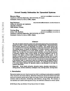
Note that (6) cannot be calculated exactly since it depends on the second derivative of p(x), and p(x) is exactly the unknown distribution we are trying to approximate. Several approaches to approximating R(p′′ (x)) have been proposed in the literature (see e.g. [9]), however these require access to all the observed samples, which is in contrast to the online learning where we wish to discard previous samples and retain only their compact representations. Our setting is depicted in Figure 1: We start from a known pdf pˆt−1 (x) from the previous time-step and in the current time-step observe a sample xt (Figure 1a). A Gaussian kernel corresponding to xt is calculated and used to update pˆt−1 (x) to yield a new pdf pˆt (x) (Figure 1b). Formally this means that the current estimate pˆt (x) is obtained as pˆt (x) = (1 −

1 1 )ˆ pt−1 (x) + Kht (x − xt ), nt nt 3

(7)

and the online kernel density estimation boils down to estimating the bandwidth ht of the Gaussian kernel for the currently observed sample xt . We can rewrite (3) by separating the kernel corresponding to the currently observed sample xt from the other kernels pˆt (x; ht ) =

(1 −

=

(1 −

nt −1 1 1 1 X ) Kht (x − xi ) + Kht (x − xt ) nt i=1 nt − 1 nt

1 1 )ˆ pt−1 (x, ht ) + Kht (x − xt ). nt nt

(8)

If we then assume that the KDE corresponding to the samples from the previous time-steps in (8) can be approximated by our estimate of the distribution from (t − 1), i.e., pˆt−1 (x, h∗ ) ≈ pˆt−1 (x) (where h∗ is the optimal choice of ht ), then the optimal bandwidth ht for pˆt (x), (7) can be approximated by the bandwidth for pˆt (x; ht ), (3). This means that, under the above assumptions, we can use (6) as a heuristic for estimating the optimal bandwidth of pˆt (x). In the following we propose an iterated plug-in rule which uses this heuristic for online bandwidth estimation. (a)

pˆt−1 (x)

(b)

pˆt (x)

xt

Figure 1: The left image shows a Gaussian mixture model pˆt−1 (x) from time-step t − 1 (bold line) and the currently observed sample xt (circle). A Gaussian kernel is centered on xt (dashed line) and used to update pˆt−1 (x). The right image shows the current, updated, mixture pˆt (x).

Let xt be the currently observed sample and let pˆt−1 (x) be an approximation to the underlying distribution p(x) from the previous time-step. The current estimate of the p(x) is initialized using the distribution ˆ t of the kernel Kˆ (x − xt ) corresponding to from the previous time-step pˆt (x) ≈ pˆt−1 (x). The bandwidth h ht the current observed sample xt is obtained by approximating the unknown distribution p(x) ≈ pˆt (x) and applying (6) √ ˆ t = [2 πR(ˆ h p′′t (x))nt ]−1/5 . (9) The resulting kernel Khˆ t (x − xt ) is then combined with pˆt−1 (x) into an improved estimate of the unknown distribution pˆt (x) = (1 −

1 1 )ˆ pt−1 (x) + Khˆ t (x − xt ). nt nt

(10)

ˆ t and Next, the improved estimate pˆt (x) from (10) is plugged back into the equation (9) to re-approximate h then equations (9) and (10) are iterated until convergence; usually, five iterations suffice. Note that with each observed sample the number of components in the mixture model increases. Therefore, in order to maintain a low complexity, a compression algorithm is initiated whenever the number of components exceeds a value Ncomp . As we will see in section 2.4 the compression (Algorithm 3) does not force removing components but merely tries to remove some. Therefore the threshold Ncomp only determines the frequency at which the compression is called. To prevent unnecessary calls to compression, the threshold Ncomp can be therefore set to some fixed large value or can be allowed to vary. In practice, we use a simple rule to adjust the Ncomp online: If no components are removed in the compression step (Algorithm 1, step 5), then Ncomp is increased, i.e., Ncomp ← cscale Ncomp , otherwise, if the number of the −1 remaining components falls below c−1 scale Ncomp , the threshold is decreased, i.e., Ncomp ← cscale Ncomp . In all the subsequent experiments, we use a scale factor cscale = 1.5. The procedure for online kernel density estimation is outlined in Algorithm 1. 4

Algorithm 1 : Online kernel density estimation Input: pˆt−1 (x), xt . . . the initial density approximation and the new sample Output: pˆt (x) . . . the new approximation of density 1: Initialize the current distribution p ˆt (x) ≈ pˆt−1 (x). ˆt (x). 2: Estimate the bandwidth ht of Kh ˆ t (x − xt ) according to (9) using p 3: Reestimate p ˆt (x) according to (10) using Khˆ t (x − xt ). 4: Iterate steps 2 and 3 until convergence. 5: If the number of components in p ˆt (x) exceeds a threshold Ncomp , compress pˆt (x) using Algorithm 3. 6: If required, adjust the threshold Ncomp . 2.2. Incorporating the negative examples In the previous section we have proposed a method for online estimation of the mixture model from all-positive examples using an online kernel density estimation. As discussed in the introduction, another important aspect of the online learning is how to account for the negative examples. This feature is especially important in real-life scenarios since it allows learning models from a noisy data and then refining these models using additional negative examples – we call this the process of unlearning. Assume that, by observing values of some feature x, we have constructed the following Mref -component Gaussian mixture model pref (x) =

M ref X i=1

wi Khi (x − xi ).

(11)

Now assume that we obtain another pdf, a Mneg -component mixture Mneg

pneg (x) =

X j=1

ηj Ksj (x − yj ),

(12)

which represents a negative example to what we want to learn. For example, we might want to learn how the hue values of red objects are distributed. pref (x) would then be a (possibly) noisy model of the red color which we have learnt sofar, and we wish to use a pdf pneg (x) estimated from the hue values of a yellow object to refine our model of the red color. The main issue in the unlearning is thus how to incorporate pneg (x) into the reference model pref (x). We can think about pneg (x) as of a pdf which specifies the likelihood by which particular values of x can be considered as a negative example to what we want to learn. A complement to pneg (x) therefore specifies another positive example, which effectively assigns low probability to those values of x which are very likely to be the negative example according to pneg (x). Thus, in summary, we propose to formulate the unlearning in the following two steps: First, we generate a so-called attenuation function fatt (x), which presents a complement to pneg (x), and maps the feature values x into interval [0, 1] by yielding 0 for the values of x where pneg (x) is maximal and 1 for the values where pneg (x) is zero. Then pneg (x) is incorporated into pref (x) simply by multiplying pref (x) with the attenuation function, yielding the attenuated mixture model patt (x). The analytical solution to this procedure is described next. The attenuation function is defined as −1 fatt (x) = 1 − Copt pneg (x),

(13)

−1 where the normalization constant Copt guarantees that Copt pneg (x) ≤ 1 and thus all values of x are mapped into the interval [0, 1]. Note that Copt corresponds to the maximum value in pneg (x) and cannot be trivially calculated, since the maximum may lay in-between the components of the mixture. For that reason we use a variable-bandwidth mean-shift algorithm [23], which we initialize at the centers of the components of pneg (x) to detect its modes. The mode xopt , corresponding to the maximum value of pneg (x), is selected as the maximum of the distribution and the normalization Copt is given as

Copt = pneg (xopt ). 5

(14)

The attenuated pdf patt (x) is obtained by multiplying the reference pdf with the attenuation function −1 −1 patt (x) = Cnorm pref (x)fatt (x) = Cnorm [pref (x) − fcom (x)],

(15)

−1 Rwhere we have defined fcom (x) = Copt pref (x)pneg (x) and Cnorm is a normalization constant such that patt (x)dx = 1. Note that since the product of two Gaussians is another, scaled, Gaussian [24], we can rewrite fcom (x) as

fcom (x) =

M neg ref M X X

Copt wi ηj Khi (x − xi )Ksj (x − µj )

M neg ref M X X

zij βij Kσij (x − µij ),

i=1 j=1

=

i=1 j=1

where zij =

√

2 σij 1 µij ( exp[ 2 2 σij 2πhi sj

−

x2i h2i

−

yj2 )], s2j

2 xi µij = σij ( h2 + i

yj ), s2j

(16)

−2 −1 2 βij = Copt wi ηj , σij = (h−2 . Now i + sj )

we can derive the normalization Cnorm for the attenuated pdf patt (x) (15) Cnorm = (1 −

XMref XMneg i=1

j=1

βij zij )−1 .

(17)

The proposed method for unlearning a mixture model is summarized in Algorithm 2. Algorithm 2 : The algorithm for unlearning mixtures Input: pref (x), pneg (x) . . . the reference mixture and the negative-example mixture. Output: patt (x) . . . the unlearned mixture. 1: Detect the location xopt of the maximum mode in pneg (x) using the variable-bandwidth mean shift [23]. 2: 3:

Scale pneg (x) with respect to the detected mode xopt (14) and calculate the attenuation function fatt (x) (13). Multiply fatt (x) with pref (x) and normalize to obtain the attenuated mixture patt (x) (15,16,17).

Note that while patt (x) is indeed a proper pdf, it is not a proper mixture model, since some of the weights are negative. Furthermore, by introducing new attenuation functions, the number of components in (15) increases exponentially, which in practice makes subsequent calculations inefficient and slow. For that reason, after the attenuation, the resulting distribution needs to be compressed, i.e., we require an equivalent mixture with a smaller number of components. Furthermore, for algorithmic reasons (because of the way in which we define the compression in the subsequent sections) it is beneficial if the equivalent is a proper mixture with all-positive weights. In the following we propose a methodology for obtaining such equivalents. 2.3. Approximating mixtures with mixtures Assume we are given a reference mixture p(x) =

M X i=1

wi Khi (x − xi ),

(18)

where all wi are not necessarily positive, but they do sum to one. Our goal is then to approximate the reference (18) with a N-component mixture with all positive weights pˆ(x|θ) =

N X j=1

γj Kσj (x − µj ), 6

(19)

where θ = {γj , µj , σj }j=1:N denotes the parameters of the mixture, such that some difference criterion between p(x) and pˆ(x|θ) is minimized. Since the reference mixture is known, the difference between the reference mixture and its approximation can be quantified by the integrated squared error (ISE) Z ISE(θ) = (p(x) − pˆ(x|θ))2 dx. (20) The problem of finding an equivalent to p(x) can thus be posed as seeking an optimal θˆ while minimizing the ISE: Z ˆ θ = arg min[ pˆ2 (x|θ)dx − 2Ep(x) {ˆ p(x|θ)}], (21) θ

where Ep(x) p(x|θ)} is the expectation with respect to the reference distribution p(x) and where we have R {ˆ dropped p2 (x)dx from the above equation since it does not depend on θ. Since we can calculate the derivatives of ISE, δISE(θ)/δθ, analytically, efficient optimization schemes such as gradient descent or LevenbergMarquardt can be used in optimizing (21). However, in practice, when M is large and N ≈ M it is likely that some components in pˆ(x|θ) will be redundant, which may result in a slow convergence of optimization. Moreover, in cases when pˆ(x|θ) is poorly initialized, optimization can get stuck in a local minimum. Therefore, a question remains how to determine the appropriate number of components in pˆ(x|θ). To address this issue, we note that component selection can be viewed as optimizing (21) with respect to the weights γi of pˆ(x|θ) (19). By driving some weights of (19) to zero we are effectively removing the corresponding components. A useful insight into such optimization is provided by the theory of the reduced-set-density estimation [25] and earlier results from the support estimation in the support vector machines [26]. In [25], Girolami and He proposed a reduced-set-density approximations of kernel density estimates. A central point of their approach was minimization of an ISE-based criterion, which is in spirit similar to our formulation in (20). In line with their observations, we now inspect how the two terms of the right-hand side of (21) affect the optimization of ISE w.r.t. the weights γi of pˆ(x|θ). If the first term of the right-hand side of (21) is kept fixed, minimization is obtained by maximizing the second term Ep(x) {ˆ p(x|θ)}. By expanding this term we have Ep(x) {ˆ p(x|θ)} = with p˜j =

R

Kσj (x − µj )[

M P

i=1

N X

γj p˜j ,

(22)

j=1

wi Khi (x − xi )]dx.

Note that (22) is a convex combination of positive numbers p˜i , which are expectations of components in pˆ(x|θ) under the reference p(x). In this case, maximization would be achieved by assigning a weight one to the largest expectation p˜j and a zero weight to all others. Thus, if the reference distribution p(x) has a dominant mode, then the component Kσj (x − µj ) of the approximating distribution pˆ(x|θ) that agrees best with this mode will be assigned a weight one, while all other weights will be zero. We say that the term Ep(x) {ˆ p(x|θ)} is sparsity-inducing in that it prefers those components of the approximating distribution pˆ(x|θ) which correspond to the high-probability regions in p(x). p(x|θ)} kept fixed equals to minimizing the first term R 2Now note that minimizing ISE (21) with Ep(x) {ˆ pˆ (x|θ)dx. Expanding this term yields a weighted sum of expectations of pairs of components of pˆ(x|θ) Z

pˆ2 (x|θ)dx =

N X N X

γi γj cij ,

(23)

i=1 j=1

R where we have defined cij = Kσi (x − µi )Kσj (x − µj )dx. The expectations among non-overlapping components will yield low values of cij , while expectations among overlapping components will yield high values of cij . In this case, ISE would be minimized by 7

assigning small weights to the overlapping components and large weights to those which do not overlap. Thus we can say that the term (23) is sparsity-inducing in that it prefers selection of those components that are far apart. From the above discussion, we can see that optimizing ISE (21) between p(x) and pˆ(x|θ) will yield a subset of components in pˆ(x|θ) by selecting components in high-probability regions of p(x), while preferring configurations in which the selected components are far apart. Using (22,23) we can rewrite the minimization of ISE (21) with respect to the weights γi into a classical quadratic program 1 arg min{ γ T Cγ − γ T P} ; γ T 1 = 1, γj > 0, ∀j, 2 γ

(24)

where 1 is a column vector of ones, and where we have defined the vector of weights γ T = [γ1 , γ2 , . . . , γN ], a symmetric N × N matrix C with elements cij (23) and a vector of P = [˜ p1 , p˜2 , . . . , p˜N ] with elements p˜j (22). Note that since all components in the reference and the approximating distributions (18,19) are Gaussians, C and P in (24) can be evaluated analytically. There is a number of optimization techniques available for solving the quadratic program (24). In our approach we use a variant of a Sequential Minimal Optimization (SMO) scheme [26], which was previously used by Girolami and He [25] for a similar optimization. 2.4. Compression algorithm Using the results from the previous section, we propose an iterative compression algorithm, which is similar in spirit to [27, 28], for finding a reduced equivalent to a reference Gaussian mixture model p(x). We start from an approximation pˆ(x|θ) which is equal to the reference mixture in cases when mixture p(x) does not contain any negative weights. When compressing the unlearned mixture, we initially increase the number of the components in the approximation by splitting each component with a negative weight into two components and then make their weights positive. This in practice makes the approximation adapt quicker to the reference distribution in regions where the reference distribution contains positive as well as negative components. After the approximation has been initialized, the components are gradually removed from pˆ(x|θ) while minimizing the ISE criterion (20) between pˆ(x|θ) and p(x). The compression algorithm proceeds in the following two steps: reduction and organization. At the reduction step, a subset of components from pˆ(x|θ) is removed using SMO. In the next step, the organization step, we further reduce the error between the reduced pˆ(x|θ) and the reference p(x). This is achieved by optimizing (21) w.r.t. all parameters θ in pˆ(x|θ) using a Levenberg-Marquardt (LM) optimization with a constraint that all weights in pˆ(x|θ) are positive. These two steps are iterated until convergence. The procedure is outlined in Algorithm 3. At each step of the iterative procedure described in Algorithm 3, a subset of components from pˆ(x|θ) is removed, thus gradually reducing the complexity of pˆ(x|θ). The number of components removed at each step can be controlled by inflating the variances of pˆ(x|θ) by some inflation parameter α > 1 before applying the SMO. For a large α, many components of pˆ(x|θ) will overlap significantly and thus many components will be removed. As a result, the final pdf pˆ(x|θ) will be a smoothed equivalent of the reference pdf p(x). However, removing too many components will increase the error in the approximation of p(x), and therefore the inflation parameter α has to be set such that the inflated pdf is always close enough to the reference pdf p(x). In our implementation, this is achieved by adjusting the α such that the Hellinger distance [29] between p(x) and the inflated pˆ(x|θ), H(p(x), pˆ(x|θ)), is always smaller than some predefined distance Hdist . Note that while the Hellinger distance is a proper metric between probability density functions and is constrained to the interval [0, 1], it cannot be calculated analytically in a closed-form for mixture models. We therefore calculate its approximation using the unscented transform [30]. For convenience, we derive the unscented approximation of the Hellinger distance for mixture models in the Appendix A. Once the selection step removes a set of components, the remaining set is optimized in order to minimize the ISE between pˆ(x|θ) and the reference p(x) (organization). Note that we do not have to optimize pˆ(x|θ) until convergence in this step. We only need to reduce the error between pˆ(x|θ) and p(x) to the extent that a set of components in pˆ(x|θ) will overlap after the inflation and will be removed in the reduction step. 8

Algorithm 3 : Compression algorithm Input: pref (x), Hdist . . . the reference mixture and the maximum allowed Hellinger distance between pref (x) and compressed counterpart. Output: pˆ(x|θ) . . . the compressed equivalent. 1: Initialization: construct p ˆ(x|θ) from p(x), such that all components have positive weights (see text). 2: Reduction: • Inflate pˆ(x|θ) into pˆα (x|θ) H(pref (x), pˆα (x|θ)) = 0.7Hdist .

by

increasing

the

variances

σj2

←

ασj2

such

that

• Optimize (24) between the inflated pˆ(x|θ) and p(x) w.r.t. γ using a SMO. • Remove those components from pˆ(x|θ) for which γi = 0. 3: 4: 5:

Organization: Optimize ISE between pˆ(x|θ) and p(x) using a LM optimization w.r.t. θ. If the distance between pref (x) and pˆ(x|θ) is small enough, i.e., H(pref (x), pˆ(x|θ)) < Hdist , then accept pˆ(x|θ) as a potential compressed equivalent. If at least one component was removed during the reduction procedure, and pˆ(x|θ)) was accepted at step (4), then go to to step (2), otherwise optimize θ until convergence and end compression.

Thus in practice we use five Levenberg-Marquardt iterations at each organization step. Only after no more components are removed, we optimize pˆ(x|θ) until convergence. 3. Experimental Results Three sets of experiments were conducted to evaluate the proposed methods for online learning and approximation of probability density functions. The first two experiments were designed to demonstrate online approximation of complex mixtures and to illustrate the concept of unlearning. In the third experiment we show how the proposed algorithms can be applied for interactive learning of basic visual properties. 3.1. Online approximation of complex distributions The aim of the first experiment was to demonstrate the performance of the online kernel density estimation proposed in Section 2.1 – we will refer to this method as an online KDE. A set of 1000 samples was generated from a reference pdf pref (x), which was a 1D mixture of a Gaussian and a uniform distribution (Figure 2a). These samples were then used one at a time to incrementally build the approximation to the original distribution using the Algorithm 1. At each time-step three other models were also built for reference. The first two were batch KDEs, and were built by processing all samples observed up to the given time-step simultaneously. In the first KDE model, we refer to it as the optimal batch KDE, the bandwidths of the kernels were estimated via solve-the-equation plug-in method [31], which is currently theoretically and empirically one of the most successful bandwidth-selection methods. In the second KDE model, we call this model a suboptimal batch KDE, the bandwidths were estimated using the Silverman’s rule-of-thumb ([9], page 60), which is a common choice of practicians. The third reference model was a Gaussian Mixture Model, which was built by applying the online Expectation Maximization (EM) coupled with model resampling and the Bayes Information Criterion [32] was used to select the number of components in the model. Since the online EM-based model requires processing data in partial batches, this model was updated using 100 samples at a time, and a maximum of 50 components was allowed in the model selection. Our online KDE was initialized using the solve-the-equation plug-in method from the first ten samples and the threshold Ncomps in the Algorithm 1 was initialized to Ncomps = 10. The online KDE was updated using only a single sample at a time. To quantify how the approximations evolve with each new sample, three different distance measures were calculated between the obtained approximations and the reference model: the integrated squared error 9

(ISE); a Hellinger distance2 ; and the log-likelihood of another set of 1000 randomly drawn samples from the reference pref (x). The distances were averaged over thirty repetitions of the experiment. Along with the distances, we have also recorded the average number of components in the approximations and for the KDE-based methods also the average bandwidth assigned to the new kernel after observing each new sample.

(a)

(d)

(b)

(c)

(e)

(f)

(g)

Figure 2: A reference mixture model (a) used in the online density approximation experiment. Approximations by online KDE with parameter Hdist set to 0.05, 0.1 and 0.3 are shown in (b), (c) and (d), respectively, the approximations obtained by suboptimal batch KDE and the optimal batch KDE are shown in (e) and (f), respectively and the approximation obtained by the online EM is shown in (g). In (b,c,d,e,f,g), the reference is drawn in dashed (blue) line and the approximations are shown by a full (red) line.

Figure 2 shows the approximations of the reference pdf after observing all 1000 samples. The approximations from the proposed online KDE with the parameter Hdist set to 0.05, 0.1 and 0.3 are shown in Figures 2(b,c,d). Recall that the parameter Hdist defines the maximal allowed error in the approximation during the compression steps. We see that for small values of Hdist , the approximations agree well with the reference pdf (Figure 2b,c). However, when Hdist was large, i.e., Hdist = 0.3, the reduction step in the compression eventually removed the components which corresponded to the low-weight uniform distribution and only retained the dominant mode (Figures 2d). In terms of the bandwidth selection, we can see from the Figure 3(a), that the proposed online KDE with parameters Hdist ∈ {0.05, 0.1} produced similar bandwidths as the optimal batch KDE, while the bandwidths of the suboptimal batch KDE were consistently over-estimated, which resulted in an over-smoothed approximation of the reference pdf (Figure 2e). Note that the graphs of the estimated bandwidths in Figure 3(a) corresponding to the online KDEs with parameters Hdist ∈ {0.05, 0.1} are virtually equal. This result is consistent with the evolution of the approximation errors in Figure 4 where we compare the online KDE with the batch KDE: while initially the errors were high for all approximations, they decreased with increasing number of samples. As expected, the error of the batch KDE calculated using Silverman’s rule remained high even after all the 1000 samples have been observed. On the other hand, the errors decreased faster for the online KDEs and came close to the errors of the optimal batch KDE with increasing number of samples. This result is consistent across all three measures of the approximation error in Figure 4. Note that the bandwidths in the optimal batch KDE were calculated using all samples observed up to a given step. In contrast, the proposed online KDEs produced similarly small errors using only a low-dimensional representations of the observed samples. This is seen in Figure 3(b) where we show the evolution of the average number of components in the approximations. In the batch KDEs (optimal and suboptimal), the complexity was increasing linearly with the observed number of samples. Thus, after observing 1000 samples, the batch KDEs were composed of 1000 kernels. On the other hand, the final approximations obtained by the proposed online KDEs with parameters Hdist = 0.1 2 The Hellinger distances between the reference distribution and its approximations were calculated by a Monte Carlo integration

10

and Hdist = 0.05 contained only 12 and 20 kernels, respectively. While the complexity of the models produced by the online KDE with Hdist = 0.05 was comparable to that of the models produced by the online EM (Figure 3b), both online KDEs consistently produced smaller errors than the online EM (Figure 5). Note that, due to the resampling step, the limited sample size and the lack of regularization in the model selection of the online EM algorithm, the resulting models sometimes contained components with nearly singular variance (see, for example, Figure 2g). The consequence of this was an increased effective number of components in the EM models. Note that, due to the resampling step, the limited sample size and the lack of regularization in the model selection of the online EM algorithm, the resulting models sometimes contained components with nearly singular variance (see, for example, Fig. 2g). The consequence of this was an increased effective number of components in the EM models. To provide an insight into the computational complexity of the online KDE, we have calculated the average times required for the model update after observing the 1000th sample in our experiment. The tests were performed with non-optimized code in Matlab [33] on a personal computer with a 2.6GHZ CPU. The times are given in Table 1. The online EM required the longest computational time, which is largely due to the model selection stages, while the suboptimal batch KDE required the shortest of computational time. The online KDEs required on average a smaller amount of processing time per update step than the optimal batch KDE. The reason si that the online KDE models have reached a bound on their complexity fairly early (after observing approximately 300 samples – see Figure 3) and therefore the processing time after observing the 1000th sample was approximately the same as if only 300 samples have been observed.

10

10

3

-1

10

num. of components

bandwidth

10

-2

-3

200

400

600

2

10

1

10

200

800

400

600

800

number of samples

number of samples

(a)

(b)

Figure 3: The graphs show how the bandwidths (a) and the number of components (b) in the KDE approximations change with increasing number of samples. The results for online KDE with Hdist 0.05 and 0.1 are depicted by bright (cyan) and dark (red) full lines. The results for the batch KDE with the optimal and suboptimal bandwidth selection are depicted by dashed (green) and dotted (blue) lines, respectively.

0.8

0.5

300

0.4

250

0.6

ISE

0.5 0.4 0.3 0.2

log-likelihood

Hellinger distance

0.7

0.3

0.2

200 150 100

0.1 50

0.1

0

0 200

400

600

800

number of samples

(a)

0

200

400

600

800

number of samples

(b)

200

400

600

800

number of samples

(c)

Figure 4: Three error measures of the KDE approximations w.r.t. the number of samples: ISE (a), Hellinger distance (b) and the log-likelihood (c). The results for online KDE with Hdist 0.05 and 0.1 are depicted by bright (cyan) and dark (red) full lines. The results for the batch KDE with the optimal and suboptimal bandwidth selection are depicted by dashed (green) and dotted (blue) lines, respectively.

11

3

10

2

1

10

0

10

-1

10

-2

log-likelihood

Hellinger distance

10

10

ISE

4

1

10

0

10

-1

10

10

10 200

400

600

800

200

number of samples

2

10

1

-2

10

3

10

400

600

200

800

(a)

400

600

800

number of samples

number of samples

(b)

(c)

Figure 5: Three error measures of the online approximations w.r.t. the number of samples: ISE (a), Hellinger distance (b) and the log-likelihood (c). The results for online KDE with Hdist 0.05 and 0.1 are depicted by bright (cyan) and dark (red) full lines, while the results for the online EM are depicted by the black dash-dotted lines.

Table 1: Average time spent per model adaptation (tspent ) after observing 1000 samples for the suboptimal batch KDE (KDEsil ), the optimal batch KDE (KDEplugin ), the online KDE with Hdist = 0.1 (OKDE0.1 ), the online KDE with Hdist = 0.05 (OKDE0.05 ) and the online Expectation Maximization with model selection oEM . (Tested on a PC with a 2.6GHz cpu)

method tspent

KDEsil 0.04s

KDEplugin 2s

OKDE0.1 0.4s

KDE0.05 1.6s

oEM 13s

From the above results we can conclude that, when Hdist parameter is set to a low value,e.g. {0.05, 0.1}, the online KDE produces approximations with smaller errors than those obtained by a suboptimal batch KDE and the online EM, while the errors are comparable to those of the batch optimal KDE . In terms of the model’s complexity, the online KDE produces models with a much lower number of components than the batch methods. While the complexity of the models is comparable to the models produced by the online EM, the online KDEs produce significantly lower errors. Therefore, with increasing the number of samples, the online KDEs converge in terms of estimation accuracy to the models produced by the batch state-of-the-art KDEs, and do so using significantly less components in their models. The reason is that the optimization (in compression as well as bandwidth selection) is not merely local in time, but is in fact distributed through time. Each new observation improves the models, bringing them closer to the optimum in terms of accuracy, while maintaining a low complexity. In the online KDE, the errors of approximation using Hdist = 0.05 and Hdist = 0.1 were virtually equal for number of samples lower than 600. As the number of samples grew, the approximation error was decreasing faster for Hdist = 0.05, however, at a cost of an increased complexity. To balance between the model complexity and approximation error, we choose Hdist = 0.1 for all our subsequent experiments. For additional examples of online estimation of probability density functions using the online KDE, see http://vicos.fri.uni-lj.si/data/matejk/ivcj08/SupplementalMaterial.htm. 3.2. Unlearning: A toy example To demonstrate how the unlearning from the Algorithm 2 can be used in interactive learning, we consider a toy-example of training a cognitive agent to learn the concept of a red color. Assume that we present the agent with an object to which we refer as a ”red fork” (Figure 6a). The agent tries to learn the concept of the red color by sampling hue values of pixels corresponding to the fork (green dots in Figure 6a) and constructs a mixture model pred (x) from the sampled values (Figure 6b). Note that two modes arise in pred (x) – one for the hue values of the red handle and one for the hue values of the yellow head. The model pred (x) can now be used to calculate a belief of whether the color of a given pixel is red or not. The beliefs of all pixels in the fork image (Figure 6a) are shown in (Figure 6h). Note that high beliefs are assigned to the color of the handle and even higher to the color of the head. Thus the agent would wrongly believe that the red as well as the yellow hues make up the concept of the red color. To rectify this we present a yellow ball (Figure 6c) and say that its color is yellow and NOT red. As before, hue values are sampled from the ball and a mixture model pyell (x) is constructed (Figure 6d). An attenuation function fatt (x) 12

a

0

0.05

e

1

c

b

0.1

d

0

0.15

g

f

0.05

h

0.1

0.15

i

0

0 0

0.05

0.1

0.15

0

0.05

0.1

0.15

0

0.05

0.1

0.15

Figure 6: Hue values are sampled from (a) to initialize the mixture model pred (x) (b). The mixture pyell (x) corresponding to the sampled hue values of a yellow ball (c) is shown in (d). The attenuation function fatt (x) is shown in (e) and the final pred (x) before and after compression is shown in (f) and (g), respectively. The belief images corresponding to pred (x) before and after unlearning, (b) and (g), are shown in (h) and (i), respectively. White colors correspond to high beliefs, while dark colors correspond to low beliefs. The mixtures in (b,d,f,g) are show in bright (red) lines, while their components are depicted in black lines.

(Figure 6e) is calculated from pyell (x) and used to unlearn the corresponding parts of pred (x); the resulting mixture is shown in (Figure 6f). After compression, we obtain the corrected model of the red color concept pˆred (x) (Figure 6g). Note that the mode corresponding to the yellow color has been attenuated, which is also verified in the belief image (Figure 6i) where we have used pˆred (x) to calculate the beliefs of hue values in (Figure 6a). The belief image shows that now only the colors of pixels on the fork’s handle are believed to correspond to the concept of the red color. 3.3. Interactive learning of basic visual concepts To further demonstrate the strength of the proposed algorithms for online learning we have embedded them into a system for continuous online learning of basic visual concepts [34]. The system operates by learning associations between six object properties (four colors and two shapes) and six low-level visual features (median hue value, eccentricity of the segmented region, etc.). Once an association (a concept) is created, a detailed model of each concept (properties-feature association) is constructed. As a testbed we have used a set of everyday objects (see Figure7a for examples). In the process of learning, a tutor presented one object at a time to the system and provided its description – the concept labels. The system created associations between features and concept labels such that, for example, the concepts of colors were associated with the hue feature. The associated visual features were modelled by KDEs using the algorithms proposed in this paper. Therefore, the concept of the green color, for example, was modelled by a KDE over the hue values of the observed green objects. In this experiment, a set of 300 images of everyday objects was randomly split in two sets of 150 images. One set was used for training and the other for testing. The images entered the learning system one by one and at every step the quality of the current models was evaluated by trying to recognize the visual properties of all testing images. The accuracy of recognition was defined as the ratio between the number of correctly recognized concepts and the number of all the concepts from the test set. The experiment was repeated 50 times with different training and test sets and the results were averaged. The evolution of the accuracy of the concept recognition is shown in Figure 7(b). It is evident that the overall accuracy increases by adding new samples. The growth of the accuracy is very rapid at the beginning, when new models of newly introduced concepts are being added, and remains positive even after all models are formed, which is due to refinement of the corresponding representations (KDEs). Note that this refinement does not come from increasing the number of components in the KDEs. This can be seen in Figure 7(c), where we show how the number of components evolved on average with new observations. Initially, the number of components is rapidly increasing, and after a while it remains approximately constant. To demonstrate the unlearning algorithm, we repeated the experiment, but now every 10-th training sample was labelled incorrectly in the first half of the incremental learning process. As a result, the underlying 13

KDE representations were corrupted by the incorrect feature values and the recognition accuracy degraded (red line in Figure 7b). However, by applying unlearning to the corrupted representations, they were successfully corrected, which resulted in a significant improvement of the recognition accuracy (blue line). The recognition results after unlearning were very similar to those obtained in an error-free learning process (compare the blue and the green line in Figure 7b). Figures 7(d-g) show an example of the evolution of the individual models over time. At the beginning, the models were very simple and rather weak, since they were obtained considering only a few training samples (Figure 7d). However, as new samples were observed, they adapted to the variability of the individual concepts. Figure 7(g) shows the models after all 150 training samples have been observed. The efficiency of the compression algorithm can be seen by inspecting columns in Figures 7(e) and (f) – most obvious compression results are seen in the second and the last column. The compressed models resemble the original ones at a very high degree. Figure 7(h) shows an example of updating the final models from Figure 7(g) by incorrectly labelled training samples. The proposed unlearning algorithm was then applied to these models by unlearning the incorrectly presented images and concepts. Figure 7(i), which depicts the obtained models, shows that the error recovery was successful and that the information that was incorrectly added into the models was successfully removed. 4. Conclusion A new approach to online estimation of Gaussian mixture models for interactive learning was proposed. The approach consists of three main contributions. The first contribution is a new approach to incremental Gaussian mixture models which allows online estimation of probability density function from the observed samples. This approach was derived by an online extension of a batch kernel density estimation (KDE). The second contribution is a method for unlearning parts of the learned mixture model, which allows for a more versatile learning. The third contribution is a method for maintaining a low complexity of the learned mixture models, a compression, which is based on iterative removal of the mixture components and minimization of the L2 distance between the original mixture and its approximation. Results of the experiments have shown that, in an online estimation of the probability density functions, a crucial part is to allow the models to have some redundant complexity, so that they can efficiently adapt to the future data. We have seen that if the errors introduced by the model compressions are kept sufficiently low, the adaptation will be successful even after observing a large number of samples. In our approach, these errors were quantified in terms of the Hellinger distance and we have proposed a numerical approximation for its evaluation between two mixture models. The performance of the online kernel density estimation (OKDE) was first demonstrated with an example of online estimation of a complex distribution from individual samples. In terms of the error between the approximations and the reference distribution, the OKDE outperformed an online EM-based mixture model, a widely-used batch KDE and produced results which were comparable to a batch state-of-the-art KDE. In contrast to the batch KDEs, where the model complexity increased with the number of samples, the OKDE maintained a low complexity even after a large number of samples have been observed. We have applied the proposed methodologies for online learning/unlearning to a tutor-supervised interactive learning of basic visual concepts in a cognitive agent. In this experiment the tutor presented the agent with an object and provided labels (concepts) associated with the objects visual properties. The agent was gradually building representations of the visual concepts using the OKDE and was able to achieve a high accuracy of recognition when the tutor provided error-free labels. When the labels contained errors, the recognition decreased, since false examples got incorporated into the models. However, using the unlearning strategy, the tutor was able to easily improve the models such that the accuracy of the recognition increased back to the level of learning with error-free labels. The methodologies proposed in this paper were designed for online estimation of models for stationary distributions (i.e., distributions which do not change in time), and have been demonstrated to allow an efficient approach to online learning in cognitive agents. In our future work we will extend this approach and apply it to other online learning problems which consider nonstationary distributions as well. Another important aspect to be further researched is the apparent nonstationarity of the distribution which can come 14

form a particular order in which the data arrive. We expect that this will have important effects on the convergence properties of the method. We have noticed in our experiments that, while the online KDEs converge to those of the batch state-of-the-art, initialization plays an important role in the rate of convergence. If the initial data points are sampled randomly from the target distribution they convey the information of the distribution’s scale, the bandwidths are initialized properly and the models converge fairly fast to the optimum estimates. However, in a pathological situation the initial data might be sampled only from a small part of the distribution. Then the initial scale would have been severely underestimated, resulting in underestimated initial bandwidths and under-smoothed distribution. During the online approximation many additional samples would have been required to remedy these effects. Another pathological situation would be the case when the bandwidths are initially severely overestimated, producing an overestimated distribution. In that situation, it is likely that the models would be initially over-compressed. Indeed, compressions which are valid at some point in time can turn out to be invalid only after many additional samples arrive. Again, more samples would be required to remedy the effects of these early compressions. The reasons for such behavior in the pathological situations is that the optimizations involved in compression and bandwidth selection produce only a locally optimal solutions. While these situations typically do not come to effect when the samples arrive randomly from a stationary distribution, we expect them to be significant when considering nonstationary distributions and ordered data. A further consideration is deriving a faster method for compressing the mixture models. Indeed, we have found that, while the bandwidth selection consumes only a fraction of the method’s processing time, the majority of the processing time is spent for compression of the mixture models. In our future work, we will also consider derivation of a faster compression method which would provide a comparable estimation accuracy. Acknowledgement This research has been supported in part by: Research program P2-0214 (RS), EU FP6-004250-IP project CoSy and EU FP7-ICT215181-IP project CogX. References [1] A. Holub, P. Perona., M. Burl, Entropy-based active learning for object recognition, in: Workshop on Online Learning for Classification, in conjunction with Conf. Comp. Vis. Pattern Recognition, 2008, pp. 1–8. [2] E. F. project, CoSy: Cognitive systems for cognitive assistants, http://www.cognitivesystems.org (2004-2008). [3] E. F. project, CogX: Cognitive systems that self-understand and self-extend, http://cogx.eu (2008-2012). [4] E. Ardizzone, A. Chella, M. Frixione, S. Gaglio, Integrating subsymbolic and symbolic processing in artificial vision, Journal of Intelligent Systems 1(4) (1992) 273–308. [5] A. M. Arsenio, Developmental learning on a humanoid robot, in: IEEE International Joint Conference On Neural Networks, 2004, pp. 3167–3172. [6] S. Kirstein, Wersing, E. H., K¨ orner, Rapid online learning of objects in a biologically motivated recognition architecture, in: 27th DAGM, 2005, pp. 301–308. [7] Online learning for classification workshop, in conjunction with IEEE Computer Society Conference on Computer Vision and Pattern Recognition (June 2007). [8] Online learning for classification workshop, in conjunction with IEEE Computer Society Conference on Computer Vision and Pattern Recognition (June 2008). [9] M. P. Wand, M. C. Jones, Kernel Smoothing, Chapman & Hall/CRC, 1995. [10] D. W. Scott, W. F. Szewczyk, From kernels to mixtures, Technometrics 43 (3) (2001) 323–335. [11] J. Goldberger, S. Roweis, Hierarchical clustering of a mixture model, in: Neural Inf. Proc. Systems, 2005, pp. 505–512. [12] K. Zhang, J. T. Kwok, Simplifying mixture models through function approximation, in: Neural Inf. Proc. Systems, 2006. [13] G. J. Mc Lachlan, T. Krishan, The EM algorithm and extensions, Wiley, 1997. [14] M. A. F. Figueiredo, A. K. Jain, Unsupervised learning of finite mixture models, IEEE Trans. Pattern Anal. Mach. Intell. 24 (3) (2002) 381–396. ˇ [15] Z. Zivkoviˇ c, F. van der Heijden, Recursive unsupervised learning of finite mixture models 26 (5) (2004) 651 – 656. [16] A. Corduneanu, C. M. Bishop, Artificial Intelligence and Statistics, Morgan Kaufmann, Los Altos, CA, 2001, Ch. Variational Bayesian model selection for mixture distributions, pp. 27–34. [17] C. A. McGrory, D. M. Titterington, Variational approximations in Bayesian model selection for finite mixture distributions, Comput. Stat. Data Analysis 51 (11) (2007) 5352–5367. [18] M. Song, H. Wang, Highly efficient incremental estimation of gaussian mixture models for online data stream clustering, in: SPIE: Intelligent Computing: Theory and Applications, 2005, pp. 174–183.

15

[19] O. Arandjelovic, R. Cipolla, Incremental learning of temporally-coherent gaussian mixture models, in: British Machine Vision Conference, 2005, pp. 759–768. [20] A. Declercq, J. H. Piater, Online learning of gaussian mixture models - a two-level approach, in: Intl.l Conf. Comp. Vis., Imaging and Comp. Graph. Theory and Applications, 2008, pp. 605–611. [21] W. F. Szewczyk, Time-evolving adaptive mixtures, Tech. rep., National Security Agency (2005). [22] B. Han, D. Comaniciu, Y. Zhu, L. S. Davis, Sequential kernel density approximation and its application to real-time visual tracking, IEEE Trans. Pattern Anal. Mach. Intell. 30 (7) (2008) 1186–1197. [23] D. Comaniciu, V. Ramesh, P. Meer, The variable bandwidth mean shift and data-driven scale selection, in: Proc. Int. Conf. Computer Vision, Vol. 1, 2001, pp. 438 – 445. [24] M. J. F. Gales, S. S. Airey, Product of gaussians for speech recognition, Computer Speech & Language 20 (1) (2004) 22–40. [25] M. Girolami, C. He, Probability density estimation from optimally condensed data samples., IEEE Trans. Pattern Anal. Mach. Intell. 25 (10) (2003) 1253–1264. [26] B. Sch¨ olkopf, J. C. Platt, J. Shawe-Taylor, A. J. Smola, R. C. Williamson, Estimating the support of a high-dimensional distribution, Neural Comp. 13 (7) (2001) 1443–1471. [27] A. Leonardis, H. Bischof, An efficient mdl-based construction of rbf networks, Neural Networks 11 (5) (1998) 963 – 973. [28] H. Bischof, A. Leonardis, View-based object representations using rbf networks, ”IVC” 19 (2001) 619–629. [29] D. E. Pollard, A user’s guide to measure theoretic probability, Cambridge University Press, 2002. [30] S. Julier, J. Uhlmann, A general method for approximating nonlinear transformations of probability distributions, Tech. rep., Department of Engineering Science, University of Oxford (1996). [31] M. C. Jones, J. S. Marron, S. J. Sheather, A brief survey of bandwidth selection for density estimation, J. Amer. Stat. Assoc. 91 (433) (1996) 401–407. [32] K. P. Burnham, D. R. Anderson, Multimodel inference: Understanding aic and bic in model selection, Sociological Methods and Research 33 (2) (2004) 261–304. [33] Matlab - the language of technical computing (2009). URL http://www.mathworks.com/products/matlab/ [34] D. Skoˇ caj, M. Kristan, A. Leonardis, Continuous learning of simple visual concepts using Incremental Kernel Density Estimation, in: International Conference on Computer Vision Theory and Applications, 2008. [35] W. H. Press, S. A. Teukolsky, W. T. Vetterling, B. P. Flannery, Numerical recipes in C (2nd ed.): the art of scientific computing, Cambridge University Press, 1992. [36] E. Veach, L. J. a. Guibas, Optimally combining sampling techniques for monte carlo rendering, in: Computer graphics and interactive techniques, 1995, pp. 419 – 428.

A. The unscented Hellinger distance In this appendix we derive a numerical approximation to the Hellinger distance between two onedimensional Gaussian mixture models p1 (x) and p2 (x) via the unscented transform. The unscented transform is a special case of a numerical integration technique called a Gaussian quadrature [35], which uses a small set of carefully placed samples to evaluate nonlinear transformations of Gaussian variables (see, e.g. [30]). The squared Hellinger distance [29] between p1 (x) and p2 (x), is defined as Z 1 1 ∆1 2 (p1 (x) 2 − p2 (x) 2 )2 dx. (25) H (p1 , p2 )= 2 Similarly to a Monte Carlo integration [36] we define an importance distribution p0 (x) = 21 p1 (x) + 12 p2 (x), which contains the support of both, p1 (x) as well as p2 (x). In our case, p0 (x) is a Gaussian mixture model N P wi Khi (x − xi ), and we rewrite (25) into of a form p0 (x) = i=1

2

H (p1 , p2 ) = = 1 2

1

1

(p1 (x) 2 − p2 (x) 2 )2 p0 (x) dx p0 (x) Z N 1X wi g(x)Khi (x − xi )dx, 2 i=1 1 2

Z

1 2 2

(26)

2 (x) ) . Note that the integrals in (26) are simply expectations over where we have defined g(x) = (p1 (x) p0−p (x) a nonlinearly transformed Gaussian random variable x, and therefore admit to the unscented transform.

16

The unscented squared Hellinger distance is thus defined as N 2 1 X X (j) (j) wi g( Xi ) Wi , H (p1 , p2 ) ≈ 2 i=1 j=0 2

(27)

where {(j) Xi , (j) Wi }j=0,1,2 are triplets of weighted sigma-points corresponding to the i-th Gaussian Khi (x − xi ), and are defined as √ (j) Xi = xi + (−1)j 1 + κhi ,  κ ; j=0 (j) 1+κ Wi = . (28) 1 ; otherwise 2(1+κ) In line with the discussion on the properties of the unscented transform in [30], we set the parameter κ to κ = 2.

17

8

100

90 7

80 6

(a)

number of components

recognition rate

70

60

50

40

30

5

4

3

20 2

correct labels corrupted labels unlearning

10

0

0

50

100

1

150

0

50

100

(c)

(b) Gr ↔Hu (6)

Cm ↔Cp (18)

150

image number

image number

Yl ↔Hu (7)

Bl ↔Hu (5)

El ↔Ec (10)

Rd ↔Hu (4)

(d)

0.018

0.306

0.595

0.655

Gr ↔Hu (15)

1.363

2.071

0.063

Cm ↔Cp (40)

0.127

0.191

0.431

Yl ↔Hu (17)

0.600

0.770

0.945

Bl ↔Hu (14)

0.982

1.019

−0.017

El ↔Ec (28)

0.021

0.059

Rd ↔Hu (21)

(e) 0.033

0.295

0.557

0.570

Gr ↔Hu (18)

1.347

2.124

−0.043

Cm ↔Cp (46)

0.118

0.279

0.372

Yl ↔Hu (19)

0.590

0.808

0.904

Bl ↔Hu (17)

0.962

1.021

−0.006

El ↔Ec (30)

0.021

0.049

Rd ↔Hu (23)

(f ) 0.033

0.295

0.557

0.527

Gr ↔Hu (29)

1.361

2.195

−0.001

Cm ↔Cp (67)

0.124

0.249

0.416

Yl ↔Hu (33)

0.609

0.803

0.904

Bl ↔Hu (36)

0.962

1.021

−0.006

El ↔Ec (57)

0.020

0.046

Rd ↔Hu (34)

(g)

−0.017

0.280

0.577

0.511

Gr ↔Hu (31)

1.341

2.171

−0.004

Cm ↔Cp (68)

0.133

0.270

0.277

Yl ↔Hu (36)

0.533

0.788

0.901

Bl ↔Hu (37)

0.964

1.027

−0.009

El ↔Ec (59)

0.019

0.047

Rd ↔Hu (36)

(h)

−0.044

0.398

0.840

0.513

Gr ↔Hu (31)

1.925

3.337

−0.013

Cm ↔Cp (68)

0.122

0.256

−0.135

Yl ↔Hu (36)

0.317

0.770

0.290

Bl ↔Hu (37)

0.659

1.027

−0.006

El ↔Ec (59)

0.019

0.044

Rd ↔Hu (36)

(i) −0.037

0.284

0.606

0.517

1.341

2.166

0.037

0.141

0.245

0.426

0.601

0.776

0.902

0.964

1.026

−0.005

0.019

0.043

Figure 7: Learning of basic object properties. Seven everyday objects from the database (a). The evolution of the recognition accuracy through time for online learning on correct data (green line), on partially incorrect data (red line), and after unlearning (blue line) (b). The average number of components through time (c). An example of the evolution of the KDE models representing six basic object properties (‘green’, ‘compact’, ‘yellow’, ‘blue’, ‘elongated’, ‘red’) through time after observing 30 (d), 80 (e), 90 (f), and 150 (g) training images. Final models updated with incorrect labels (h). Models after unlearning (i).

18