Sparse Modeling and Recursive Prediction of Space-Time Dynamics in Stochastic Sensor Networks Yun Chen and Hui Yang*, Member, IEEE
networked through wireless links, deployed in large numbers and distributed throughout complex physical systems [1]. Distributed sensing provides an unprecedented opportunity to monitor space-time dynamics of complex systems and to improve the quality and integrity of operation and services. Also, distributed sensing is widely used to improve the quality of life in healthcare systems. Wireless sensor network shows a significant capability to improve the healthcare services and realize the smart health of chronically ill and elderly. Body area sensor network [2] is the ad hoc network of sensors (e.g., RFID tags, electrocardiogram (ECG) sensors, and accelerometers) that people can carry on their body. Fig. 1 shows the wearable ECG sensor network that provides high-resolution sensing of cardiac electrical dynamics [3]. Prior research showed that high-resolution ECG mapping substantially enhances the early detection of life-threatening events for cardiovascular patients [4, 5]. When continuously monitored and analyzed, wearable ECG sensor network offers an unprecedented opportunity to realize smart care of patients with high risks (e.g., acute cardiac events) beyond the confines of, often high-end healthcare settings, and allow rural care centers to acquire sophisticated imaging and diagnostic capability at a fraction of capital investments.
Abstract—Wireless sensor network has emerged as a key technology for monitoring space-time dynamics of complex systems, e.g., environmental sensor network, battlefield surveillance network, and body area sensor network. However, sensor failures are not uncommon in traditional sensing systems. As such, we propose the design of stochastic sensor networks to allow a subset of sensors at varying locations within the network to transmit dynamic information intermittently. Realizing the full potential of stochastic sensor network hinges on the development of novel information-processing algorithms to support the design and exploit the uncertain information for decision making. This paper presents a new approach of sparse particle filtering to model spatiotemporal dynamics of big data in the stochastic sensor network. Notably, we developed a sparse kernel-weighted regression model to achieve a parsimonious representation of spatial patterns. Further, the parameters of spatial model are transformed into a reduced-dimension space, and thereby sequentially updated with the recursive Bayesian estimation when new sensor observations are available over time. Therefore, spatial and temporal processes closely interact with each other. Experimental results on real-world data and different scenarios of stochastic sensor networks (i.e., spatially, temporally, and spatiotemporally dynamic networks) demonstrated the effectiveness of sparse particle filtering to support the stochastic design and harness the uncertain information for modeling space-time dynamics of complex systems.
Back View
Front View
Note to Practitioners—This paper is motivated by a new idea of stochastic sensor networks to realize highly resilient sensing systems. The new system allows a random subset of sensors to transmit information intermittently at dynamically varying locations within the network of sensors, but calls for the development of novel analytical methodology for information processing under uncertainty. This paper presents a novel approach of sparse particle filtering to model spatiotemporal dynamics of big data in stochastic sensor networks. Experimental results demonstrated model effectiveness and robustness to support the design of stochastic sensor network.
(a)
(b)
Fig. 1. Body area ECG sensor network. (a) Front view. (b) Back view. (Note: black dots represent sensor locations.)
However, it is not uncommon to encounter sensor failures in traditional sensor networks. For example, a subset of sensors often lose contact with the skin surface in ECG sensor networks because of body movements (see Fig. 1). Maintaining strict skin contacts for hundreds of sensors is not only challenging but also greatly deteriorates the wearability of ECG sensor networks. Therefore, we propose a novel strategy, named “stochastic sensor network”, that allows a subset of sensors at varying locations within the network to transmit dynamic information intermittently. Notably, the new strategy of stochastic sensor networks is generally applicable in many other domains. For examples, wireless sensor network is often constrained by finite energy resources. Hence, optimal scheduling of activation and inactivation of sensors is imperative to realize long-term survivability and reliability of sensor networks. In addition, a subset of sensor nodes in a battlefield surveillance network may need to enter dormant states to avoid the reconnaissance from the enemy, but others
Index Terms—Stochastic sensor network, sparse particle filtering, spatiotemporal modeling, resilient sensing systems
I. INTRODUCTION
W
ireless sensor network has emerged as a key technology to monitor nonlinear stochastic dynamics of complex systems. Recent advancements in wireless communication and electronics have improved the design and development of wireless sensors that are miniature, low-cost, low-power and multi-functional. These inexpensive sensors can be easily This work is supported in part by the National Science Foundation (CMMI-1454012, CMMI-1266331, IIP-1447289 and IOS-1146882). Yun Chen is with the Complex Systems Monitoring, Modeling and Analysis laboratory, University of South Florida, Tampa, FL 33620 USA Hui Yang* is with the Harold and Inge Marcus Department of Industrial and Manufacturing Engineering, The Pennsylvania State University, University Park, PA 16802 USA, (e-mail of corresponding author:
[email protected]).
1
surface, thereby adversely affecting wearability – which has been a stumbling block to widespread applications of ECG sensor networks from research laboratory to healthcare settings. As the movement of human body is highly dynamic, few, if any, previous studies have considered the new design of stochastic ECG sensor network that allows stochastic sensor-skin contacts. As such, a subset of ECG electrodes will capture cardiac electrical activity intermittently at dynamically varying locations within the network. However, if we lower the hardware requirement on sensor-skin contacts, new analytical algorithms are urgently needed to support the stochastic design and handle data uncertainty. Notably, this new idea of stochastic sensor network received few attention in the past, partly due to traditional designs that sacrifice the wearability for data quality, and partly to the lack of analytical algorithms for spatiotemporal data modeling under uncertainty. These gaps pose significant technological barriers for realizing the design of stochastic sensor network. Fig. 2 is an illustration of spatiotemporal data generated from the distributed sensing. Each cross-section represents a snapshot of the underlying complex process at a specific time. As the dynamics of complex systems vary across both space and time, sensor networks give rise to spatiotemporal data: {Y(𝒔, 𝑡): 𝒔 ∈ 𝑅 ⊂ ℝ𝑑 , 𝑡 ∈ 𝑇}, where the dependence of spatial domain R on time T symbolizes the changes of spatial domain over time. Traditionally, spatiotemporal data is characterized and modeled in two ways: (𝑖) spatially-varying time series model 𝑌(𝒔, 𝑡) = 𝑌𝒔 (𝑡), which separates the temporal analysis for each location; (𝑖𝑖) temporally-varying spatial model 𝑌(𝒔, 𝑡) = 𝑌𝑡 (𝒔), which separates spatial analysis for each time point. The first model 𝑌𝒔 (𝑡) shows specific interests in time-dependent patterns for each sensor, and allows for sensor-to-sensor analysis between time series. For example, Yang et al. studied ECG time series and exploited the useful information for medical decision making [6-9]. The second model 𝑌𝑡 (𝒔) focuses more on space-dependent patterns for each time point. For example, Zarychta et al. studied spatial patterns in each ECG image for the detection of myocardial infarctions [10]. However, both approaches are conditional methods studying either the space given time or time given space, and are limited in their capabilities to characterize and model space-time correlations. Space-time interactions bring substantial complexity in the scope of modeling, because of spatial correlation, temporal correlation, as well as how space and time interact. Notably, many previous works employed random fields in ℝd+1 to model space and time dependencies [11, 12]. However, space and time are not directly comparable, because space does not have the past, present, and future and the spatial dimension is not comparable to temporal dimension. In the past few years, spatiotemporal modeling has received increased attentions due to the proliferation of data sets that are varying both spatially and temporally. Examples of application areas include brain imaging [13, 14], manufacturing [15], environment [16, 17], public health [18, 19], service equity [20] and socio-economics [21]. The specific questions include the analysis of time-varying brain image and fMRI data, nanowire growth modeling at multiple spatial scales, temporal movement of hurricane, geographical diffusion of pandemic infectious diseases, and spatial equity of public services.
continue working to detect real-time battlefield information. The locations of dormant sensors may also be stochastically varying so as to save energy and build a robust network for information visibility. Realizing the full potential of stochastic sensor network hinges on the development of novel information-processing algorithms to support the design and exploit the uncertain information for decision making. Real-time distributed sensing generates spatially-temporally big data, which contains rich information of evolving dynamics of complex systems. Further, stochastic sensor network brings greater levels of uncertainty and complexity which pose significant challenges for information extraction and decision making. This paper presents a new approach of sparse particle filtering to model spatiotemporal dynamics in the big data from the stochastic sensor network. We first leverage the cross-section data (e.g., time t i in Fig. 2) to develop a sparse kernel-weighted regression model to achieve a parsimonious representation of spatial patterns. Further, the parameters of spatial model are transformed into a reduced-dimension space, and thereby sequentially updated with the recursive Bayesian estimation when new sensor observations are available at time t i+1 . Thus, spatial and temporal processes closely interact with each other. Experimental results on different scenarios of stochastic sensor networks (i.e., spatially, temporally, and spatiotemporally dynamic networks) show the effectiveness of sparse particle filtering to support the stochastic design and harness the uncertain information for decision making. Temporal dynamic evolution
Spatial correlation 𝑌(𝒔, 𝒕) 𝒕𝟏
𝒕𝟐
…
𝒕𝑻
Time
Fig. 2. Space-time data generated from distributed sensor network.
This paper is organized as follows: Section II presents the research background. Section III introduces the research methodology. Section IV presents materials and experimental design. Section V presents experimental results, and Section VI discusses and concludes this investigation. II. RESEARCH BACKGROUND Wireless sensor network has broad applications in healthcare, environment, logistics, defense and many other areas. However, very little work has been done to design the stochastic sensor network and further develop new analytical methodologies to exploit spatiotemporal data for information extraction and knowledge discovery. For example, ECG sensor network has the promise to provide high-resolution sensing of space-time cardiac electrical dynamics (see Fig. 1). However, there are remarkable impetuses towards the use of wearable ECG systems to monitor cardiac activity in the past few decades. The ECG sensor network uses hundreds of electrodes to obtain electrical measurements on the body surface. Each electrode is required to maintain rigid contact with the skin
2
However, very little work has been done to realize a highly resilient sensor network by developing new spatiotemporal algorithms. Traditional spatiotemporal methods are not concerned with the uncertainty in stochastic sensor network but rather assume reliable sensor readings at fixed locations. For example, brain imaging data are homogeneous and synchronized in time for every pixel, but stochastic sensor networks involves heterogeneous data that are asynchronized and incomplete at dynamically-varying locations of the network. Therefore, this present investigation aims to develop new algorithms to realize a highly resilient sensing system, namely stochastic sensor network. Such a resilient sensing system will reduce the requirement in sensor reliability, handle data uncertainty and heterogeneity, and enable fast and recursive prediction of space-time information.
As shown in Fig. 4, the observations of body area sensor network in the front and back of the body are varying with respect to time. At a given time point, the approach here is to capture the spatial correlation in distributed sensor networks as a model of the form 𝑁
𝑌(𝒔) = 𝑀(𝒔; 𝜷) + 𝜀(𝒔) = ∑ 𝑤𝑖 (𝒔)𝒇𝑇𝑖 (𝒔)𝜷𝑖 + 𝜀(𝒔)
where Y(𝐬) is an observation taken at the location 𝐬 in the body surface, N is the total number of kernel components, and ε(𝐬) is the Gaussian random noises. The wi (𝐬) is a non-negative weighting kernel, i.e., 1
𝑤𝑖 (𝒔) ∝ |𝜮𝑖 |−2 exp {−
This paper presents the first-of-its-kind technology of stochastic sensor network in the application of body area sensor network for wearable ECG sensing, which has been granted a US Patent (US9014795 B1). We developed a new approach of sparse particle filtering to characterize and model distributed sensing data that are non-homogeneous, asynchronized and incomplete. As shown in Fig. 3, the proposed stochastic sensor network is supported by the algorithms of sparse particle filtering and optimal kernel placement. First, a state space formulation is utilized to model spatiotemporal dynamic data generated by the stochastic sensor network. Second, an optimal kernel placement algorithm is developed to improve the compactness of kernel-weighted regression model of spatial patterns. In other words, we aims to minimize the number of kernels used for spatial representation. Third, we developed the new approach of sparse particle filtering model to reduce the dimensionality of parameters in spatial model and sequentially update the parameters when new observations are available at the next time point, thereby effectively modeling space-time dynamic data generated from stochastic sensor networks.
(2)
𝑇
body area sensor network. The 𝒇𝒊 (𝒔) = (𝑓𝑖1 (𝒔), ⋯ , 𝑓𝑖𝑝 (𝒔)) is a set of known basis functions, e.g., 𝒇𝑖 (𝒔) = (1, 𝑥, 𝑦)𝑇 in this present investigation. Here, 𝑥, 𝑦 are the spatial coordinates of the location 𝐬 . Notably, 𝛃i = (βi1 , … , βip )𝑇 is a vector of model parameters. The dimensionality of 𝜷 is 𝑁 × 𝑝, i.e., the multiplication of the number of kernels 𝑤𝑖 (i.e., 𝑁) and the number of basis functions 𝒇𝑖 (i.e., 𝑝). …
…
𝑴(𝒔; 𝜷𝑡1 ) + 𝜺
𝑴(𝒔; 𝜷𝑡3 ) + 𝜺
𝑴(𝒔; 𝜷𝑡2 ) + 𝜺
Fig. 4. Time-varying ECG imaging on the body surface.
Stochastic Sensor Network
Note that the spatial model is designed as a locally weighted mixture of kernel regressions. If we observe 𝐘 = 𝑇 (Y(𝐬1 ), … , Y(𝐬K )) for locations 𝐬1 , … , 𝐬K at a specific time point, the model can be written in a matrix form as:
Space-Time Dynamic Data State Space Model
𝑌(𝒔1 ) ⋮ ] = Ψ𝜷 + 𝜺 = 𝑌(𝒔𝐾 ) 𝑤1 𝑓11 |𝒔1 ⋯ 𝑤1 𝑓1p |𝒔1 ⋯ 𝑤1 𝑓11 |𝒔2 𝑤1 𝑓1p |𝒔2 ⋮ ⋮ ⋮ ⋱ [𝑤1 𝑓11 |𝒔𝐾 ⋯ 𝑤1 𝑓1p |𝒔𝐾 ⋯
𝑌(𝒔, 𝑡) = 𝑴(𝒔; 𝜷𝑡 ) + 𝜀
(3)
𝒀=[
𝑁
∑ 𝑤𝑖 (𝒔)𝒇𝑻𝑖 (𝒔)𝜷𝒊,𝑡 𝑖=1
NLPCA: 𝒁1:𝑡 = Φ(𝜷1:𝑡 ) Particle Filtering: 𝒁𝑡 = 𝒉𝑡 (𝒁𝑡−1, 𝝎)
Sparse Particle Filtering
(𝒔 − 𝝁𝑖 )𝑇 𝜮−1 𝑖 (𝒔 − 𝝁𝑖 ) } 2
where 𝝁𝑖 is the center and 𝜮𝑖 is the covariance function of the 𝑖𝑡ℎ kernel component. Here, the weighting kernel is not limited to be Gaussian kernel. We choose the Gaussian kernel because the Gaussian kernel is the most widely used kernel function. Without loss of generality, we choose Gaussian function as the kernel in the spatial model to demonstrate the methodology. In addition, the shape of Gaussian function is similar to the local pattern of real-world ECG waveforms, which is recorded with
III. RESEARCH METHODOLOGY
𝑴(𝒔; 𝜷𝑡 ) =
(1)
𝑖=1
Optimal Kernel Placement
𝑤𝑁 𝑓𝑁1 |𝒔1 𝑤𝑁 𝑓𝑁1 |𝒔2 ⋮ 𝑤𝑁 𝑓𝑁1 |𝒔𝐾
⋯
𝑤𝑁 𝑓𝑁p |𝒔1 𝑤𝑁 𝑓𝑁p |𝒔2 ⋮
𝛽11 𝛽12 𝛽13 + 𝜺 ⋮ ⋮ ⋯ 𝑤𝑁 𝑓𝑁p |𝒔𝐾 ] [𝛽𝑁𝑝 ]
Once the observed locations 𝒔𝟏 , … , 𝒔𝑲 and kernel components 𝑤𝑖 , 𝑖 = 1, … , N are determined, the matrix Ψ is determined. Therefore, the model parameters 𝛃 can be estimated by solving the function 𝐘 = 𝚿𝛃 + 𝛆. For an unobserved location 𝐬̃ , we ̃ 𝛃 giving the known observations can predict Y(𝐬̃) as 𝚿 Y(𝐬1 ), … , Y(𝐬K ) at distributed locations. Notably, this is the kernel-weighted regression model of spatial data at a specific time point. To consider temporal dynamic effects, we augment the spatial model to include temporal components, i.e., defining the time-varying model
Fig. 3. Flow chart of research methodology.
A. Spatial Modeling It is well known that two sensors in the distributed sensor network tend to have a stronger correlation when they are closer to each other. Therefore, the spatial correlation between neighboring sensors is critical to estimate the observations of distributed sensors at a given time point.
3
𝑇
𝑇 objective function is ℛ(𝒜) = ‖𝒀 − ∑𝑁 𝑖=1 𝑤𝑖 (𝜽𝒊 )𝒇𝑖 𝜷𝑖 ‖ with two important and intuitive properties: 1) Monotonicity: ℛ(𝒜) ≤ ℛ(ℬ) for all 𝒜 ⊆ ℬ . Hence, adding kernels decreases the objective function. 2) Submodularity: Adding a new kernel to a small kernel set 𝒜 provides more advantage than adding it to a larger kernel set ℬ ⊇ 𝒜 . In other words, for a new kernel with the parameter 𝜽 ∉ ℬ ⊇ 𝒜, it holds that ℛ(𝒜) − ℛ(𝒜⋃{𝜽}) ≥ ℛ(ℬ) − ℛ(ℬ⋃{𝜽}).
parameters as 𝛃𝐭 = (𝛽11 , … , 𝛽1𝑝 , … , 𝛽𝑁1 , … , 𝛽𝑁𝑝 )𝑡 at time t . As shown in Fig. 4, as distributed sensor observations are varying in both space and time, model parameters vary with respect to time, i.e., M(s; 𝛃𝐭 ), M(s; 𝛃𝐭+𝟏 ), ⋯. Then, we develop a particle filter to establish temporal correlation to recursively estimate the state of parameters, i.e., link the parameters 𝛃t over time by the evolution equation: (4) 𝜷𝑡 = 𝑔𝑡 (𝜷𝑡−1 , 𝛾) where g t is the nonlinear evolution model and γ is process noise. Thus, the spatial model at a given time is defined as: (5) 𝒀𝑡 = 𝜳𝑡 𝜷𝑡 + 𝜀 The temporal filter is responsible for projecting forward (in time) current estimates of state and error covariance to obtain the estimates for the next time step. The spatial update is responsible for the feedback, i.e., incorporating new observations to derive posterior estimations. Although the temporal part is conceptually similar to general filtering approaches in time series analysis, the difference is that spatial and temporal processes closely interact with each other.
Initialization: Θ = {𝜽|(𝝁, 𝚺)} // search space 𝒜=∅ // selected set of kernels 𝑖=1 While 𝑖 ≤ 𝑁 𝑇 𝑇 ℛ(𝒜⋃{𝜽}) = 𝒀 − (∑𝑖−1 𝑗=1 𝑤𝑗 (𝜽𝑗 )𝒇𝑗 𝜷𝑗 + 𝑤(𝜽)𝒇 𝜷) 𝜽𝑖 = argmax ℛ(𝒜) − ℛ(𝒜⋃{𝜽}) 𝜽∈Θ
//the 𝑖th selected kernel location ̂ /𝜕𝜮] 𝑱 = [𝜕𝒀 //Jacobian matrix // Levenberg-Marquardt update of covariance function ̂ (Σ i )) ∆Σ i = [𝑱𝑇 𝑱 + 𝜆diag(𝑱𝑇 𝑱)]−1 𝑱𝑇 (𝒀 − 𝒀 Σ i+1 = Σ i + ∆Σ i until convergence // Update the selected set of kernels 𝒜 = 𝒜 ∪ {𝜽𝑖 } Θ = Θ\{𝜽𝑖 } 𝑖 =𝑖+1
However, there are two practical issues pertinent to the construction of spatiotemporal models. (1) How to optimally place kernels in the design space? Traditionally, kernels are uniformly distributed in the space. However, this unavoidably leads to a very complex model. The objective here is to identify a parsimonious set of kernels that are sufficient to achieve optimal model performances. Section III.B will detail our developed algorithms for optimal kernel placement. (2) How to identify latent variables and establish the reduced-dimension particle filtering? It may be noted that the dimensionality of parameters 𝜷𝑡 is large, and the 𝛃′s have certain nonlinear-correlation structures. In particular, sensor observations are highly nonlinear and non-stationary in both spatial and temporal domains. The objective here is to identify a compact set of independent latent variables that suffice to represent the nonlinear dynamic process of temporal parameter variations. Section III.C will detail the developed sparse particle filtering model.
End Fig. 5. Optimal kernel placement algorithm.
As a result, the problem of optimal kernel placement is reduced to the minimization of submodular functions, subject to the constraint on a sparse set of kernels. Minimizing the submodular function is well-known to be NP-hard [22]. The greedy algorithm is a commonly used heuristic, which starts with the empty set 𝒜 = ∅, and iteratively adds the new kernel 𝑤(𝜽𝑖 ), 𝒜 = 𝒜 ∪ {𝜽𝑖 } that maximizes the marginal benefit: 𝜽𝑖 = argmax ℛ(𝒜) − ℛ(𝒜⋃{𝜽}) (7) 𝜽∈Θ\𝒜
The algorithm stops when 𝑁 kernels are selected. For each kernel location 𝝁, the covariance matrix 𝚺 is further fine-tuned to maximize the marginal benefit. Here, we adopted the Levenberg-Marquardt update [23] to optimize the covariance matrix 𝚺 that minimizes the sum of squared errors between the data {𝑌(𝒔𝑘 , 𝑡)} and the model output {𝑌̂(𝒔𝑘 , 𝑡; 𝚺)}as:
B. Optimal Kernel Placement The objective of optimal kernel placement is to identify a compact set of kernels that minimize the representation error:
𝐾
argmin𝑁 [‖𝒀(𝑠, 𝑡) − ∑ 𝑤𝑖 (𝑠, 𝜽𝒊 )𝒇𝑇𝑖 (𝑠)𝜷𝑖 (𝑡)‖ , {𝜽𝒊 } ]
𝑇
2 1 𝜒 = ∑ ∑ (𝑌(𝒔𝑘 , 𝑡) − 𝑌̂ (𝒔𝑘 , 𝑡; 𝚺)) 2 (8) 𝑘=1 𝑡=1 1 𝑇 1 𝑇 𝑇̂ ̂ 𝒀 ̂ = 𝒀 𝒀−𝒀 𝒀+ 𝒀 2 2 The gradient of the sum of squared errors with respect to the parameters is: 𝑇 𝜕 𝑇 𝜕 2 𝜒 = (𝑌 − 𝑌̂(𝜮)) (𝑌 − 𝑌̂(𝜮)) = − (𝑌 − 𝑌̂(𝜮)) 𝐽 𝜕𝜮 𝜕𝜮 (9) 𝐽 = [𝜕𝑌̂/𝜕𝜮] where the Jacobian matrix represents the local sensitivity of the model to variations of covariance parameters. The Levenberg-Marquardt method adaptively updates the covariance parameters with the perturbation ∆𝚺 between the gradient descent and Gauss-Newton update. (10) ∆𝜮 = [𝐽𝑇 𝐽 + 𝜆diag(𝐽𝑇 𝐽)]−1 𝐽𝑇 (𝑌 − 𝑌̂(𝜮))
𝑁
2 (𝚺)
(6)
𝑖=1
In equation (2), it may be noted that each kernel 𝑤𝑖 (𝜽𝒊 ) contains free parameters 𝜽𝒊 = (𝝁𝑖 , 𝜮𝑖 ), where 𝝁𝑖 is the center and 𝜮𝑖 is the covariance function, i.e., 𝜮𝑖 = σ2𝑥 (𝑖) 𝜌(𝑖)𝜎𝑥 (𝑖)𝜎𝑦 (𝑖) [ ] . In total, there are five 𝜌(𝑖)𝜎𝑥 (𝑖)𝜎𝑦 (𝑖) σ2𝑦 (𝑖) parameters for each kernel 𝑤𝑖 (𝜽𝒊 ) , i.e., 𝜽𝒊 = {𝜇𝑥 (𝑖), 𝜇𝑦 (𝑖), 𝜌(𝑖), 𝜎𝑥 (𝑖), 𝜎𝑦 (𝑖)}. In order to identify a sparse set of kernels, we developed the greedy search algorithm to optimally select the kernel center (𝜇𝑥 (𝑖), 𝜇𝑦 (𝑖)) in the search space, and then fine-tune the covariance matrix 𝜮𝑖 at the chosen location by Levenberg-Marquardt method. Fig. 5 shows the algorithm of optimal kernel placement. First, we define the search space of kernels as Θ = {(𝝁, 𝚺)}, and 𝒜 = {𝜽𝒊 }𝑁 𝑖=1 ⊂ Θ is the selected set of kernels. The 4
𝑝(𝑌𝑡 |𝛃𝑡 ), based on the available observations 𝒀1:𝑡 up to time 𝑡 and the prior distribution of 𝑝(𝛃𝑡 |𝑌1:𝑡−1 ), 2) Prediction: When the posterior distribution of 𝑝(𝛃𝑡 |𝑌1:𝑡 ) is obtained via the estimation step, the parameters at the next time point 𝛃𝑡+1 can be predicted conditionally on present observations 𝒀1:𝑡 as
where λ is the learning rate. The learning process stops when convergence is achieved with the following three criteria: (1) Convergence in parameters, max(|∆𝚺 i ⁄𝚺 i |) < ϵ ; (2) ̂(𝚺))|) < ϵ; (3) Convergence in the gradient, max (|𝐽 𝑇 (Y − Y Convergence in χ2 (𝚺), χ2 < ϵ. However, the greedy algorithm is very expensive for a large search space Θ. Therefore, we exploit the submodularity of the objective function ℛ(𝒜) to achieve a scaling-up implementation, namely “lazy” greedy algorithm [24]. Initially, we compute the marginal benefit as δ(𝛉) = ℛ(𝒜) − ℛ(𝒜⋃{𝛉}), and construct a priority heap structure. At each iteration, the kernel with the largest benefit is popped from the heap and included in 𝒜. The inclusion of this kernel affects the benefits of the remaining kernels in the heap. The traditional way is to update the heap at each iteration. However, due to the submodular property, a more efficient way is to only update the marginal benefit of the top kernel in the heap. Therefore, we update the benefit of the top kernel 𝑤(𝛉∗ ) as δ(𝛉∗ ) = ℛ(𝒜) − ℛ(𝒜⋃{𝛉∗ }) in each iteration, and compared with the benefits of all kernels in the heap. If δ(𝛉∗ ) remains to be the largest benefit among δ(𝛉), 𝛉 ∈ Θ\𝒜 , then it will be selected. Otherwise, δ(𝛉∗ ) will be moved downward in the priority heap and the benefit of the next top kernel will be recalculated. As such, a compact set of kernels are sequentially selected to minimize the representation error. Notably, the “lazy” greedy algorithm does not require the update of marginal benefits for all kernels in the heap at every iteration. In addition, it enables the selection of an optimal kernel with the largest marginal benefit through a “lazy” evaluation of objective function ℛ(𝒜) . The integration of “lazy” greedy algorithm with Levenberg-Marquardt method effectively maximizes the marginal benefit δ(θ) = ℛ(𝒜) − ℛ(𝒜⋃{𝛉}) in each iteration of the learning process.
𝑝(𝛃𝑡+1 |𝒀1:𝑡 ) = ∫ 𝑝(𝛃𝑡+1 |𝛃𝑡 )𝑝(𝛃𝑡 |𝒀1:𝑡 ) 𝑑𝛃𝑡
(13)
As such, the parameters 𝛃t+1 at time point t + 1 can be predicted based on observations Y1:t , which provides the prior probability p(𝛃t+1 |Y1:t ) for the estimation step. However, the computation in spatiotemporal modeling equations (11-13) poses significant challenges: 1) Nonlinear and non-Gaussian properties: It is not uncommon that spatiotemporal data from distributed sensing of complex systems are highly nonlinear and nonstationary. Hence, the function 𝜷𝑡 = 𝑔𝑡 (𝜷𝑡−1 , 𝛾) is in a nonlinear form and 𝑝(𝛃𝑡 |𝒀1:𝑡 ) is a non-Gaussian distribution. Traditional methods, e.g., Kalman filter (KF), are only effective when the state space model is linear and the posterior density follows a Gaussian distribution. If these assumptions are not satisfied, KF uses linear approximation of nonlinear problems. Such an approximation may not yield good performance in this case. Therefore, we propose the particle filter (PF) to recursively compute estimation and prediction steps, and approximate the posterior distribution of states with a large number of particles generated by sequential Monte Carlo sampling. As shown in Fig. 6, particle filtering represents the multimodal distribution by drawing a large number of samples from it, so that the density of samples in one area of the state space represents the probability of that region. As the number of particles increases, the Monte Carlo characterization is analogous to the usual functional description of posterior distribution. Particle filtering has the advantage to represent any arbitrary complex distribution, and is effective for non-Gaussian, multi-modal distributions.
C. Sparse Particle Filtering As shown in Section III.A, the spatiotemporal model is formulated as: 𝐘t (𝐬) = 𝚿t (𝐬)𝛃t + ε (11) 𝜷𝑡 = 𝑔𝑡 (𝜷𝑡−1 , 𝛾) The alternative probabilistic representation of this model is 𝑝(𝒀𝑡 |𝛃𝑡 ) for the observation equation and 𝑝(𝛃𝑡 |𝛃𝑡−1 ) for the equation of parameter evolution. When new observations 𝑌𝑡 are available from the distributed sensor network, 𝑝(𝛃𝑡 |𝒀𝑡 ) can be estimated based on the Bayesian theory. Further, the parameters 𝛃𝑡+1 at the next time point can be predicted based on the equation of parameter evolution. The particle filtering includes two sequential steps. The estimation step provides the posterior probability p(𝛃t |Y1:t ) , while the prediction step provides the prior probability p(𝛃t+1 |Y1:t ) for the estimation step. This process is recursively updated over time: 1) Estimation: The posterior density estimation of 𝑝(𝛃𝑡 |𝒀𝑡 ) via Bayesian theory is represented as 𝑝(𝑌𝑡 |𝛃𝑡 ) (12) 𝑝(𝛃𝑡 |𝑌1:𝑡 ) = 𝑝(𝛃𝑡 |𝑌1:𝑡−1 ) 𝑝(𝑌𝑡 |𝑌1:𝑡−1 ) where 𝑝(𝑌𝑡 |𝛃𝑡 ) provides the likelihood for observation 𝑌𝑡 given parameters 𝛃𝑡 . The posterior distribution of parameters 𝑝(𝛃𝑡 |𝑌1:𝑡 ) is estimated by maximizing the likelihood function
Fig. 6. Representation of multi-modal distribution using importance sampling.
2) Curse of dimensionality: It is also important to note that the dimensionality of parameter vector, 𝛃= (𝛽11 , … , 𝛽1𝑝 , … , 𝛽𝑁1 , … , 𝛽𝑁𝑝 ) is very large. If 𝑁 kernels 𝑤𝑖 (𝒔) and 𝑝 basis functions 𝒇𝑖 (𝒔) are used in the spatiotemporal model, the dimensionality of 𝛃 is 𝑁 × 𝑝, i.e., the multiplication of number of kernels and number of basis functions. This creates a serious “curse of dimensionality” problem for estimation and prediction steps in particle filtering. The high-dimensional states will easily cause both overfitting and ill-posed estimation problems. In particular, the 𝛃′s have certain nonlinear-correlation structures. Now, an immediate question becomes “Can we identify a compact set of latent state variables from the high-dimensional parameter space, and
5
a1 a2 aτ + + ⋯+ +c 1 + e−b1𝐙t 1 + e−b2𝐙t−1 1 + e−bτ𝐙t−τ+1 where 𝜏 is the time lag, and 𝛗 = (a1 , … , a τ , b1 , … , bτ , c) are model parameters. To this end, we integrate the sequential Monte Carlo method with Kernel smoothing approach [26-28] to simultaneously estimate model states 𝐙t+1 and model parameters 𝛗. Note that Bayesian theory provides the joint distribution as p(𝐙𝐭+𝟏 , 𝛗𝒕+𝟏 |Y1:t+1 ) (15) = p(Yt+1 |𝐙𝐭+𝟏 , 𝛗𝒕+𝟏 )p(𝐙t+1 |𝛗𝒕+𝟏 , Y1:t )p(𝛗𝑡+1 |Y1:t )
thereby constructing a sparse particle filtering model of the nonlinear dynamic process?” Notably, very little work has been done to develop a sparse particle filtering model that identifies a compact set of independent states that suffice to represent the nonlinear dynamic process. Prior research on particle filtering is limited in its capability in identifying latent factors. Principal component analysis (PCA) decomposes high-dimensional variables Y into linearly uncorrelated sources Z through a linear mapping A, i.e., 𝑌 = 𝐴𝑍 + 𝑣. However, PCA is only capable of delineating linear components, and often fails to handle nonlinear correlation structures in high-dimensional variables. In addition, traditional PCA methods do not account for the dynamics of hidden factors even though complex systems evolve dynamically. In this present investigation, we integrated the nonlinear PCA (NLPCA) with particle filtering for modeling space-time dynamics in distributed sensor networks. The NLPCA generalizes the principal components from straight lines to curves and thereby captures inherent structures of the nonlinear data by curved subspaces. As shown in Fig. 7, instead of directly modeling the parameters 𝛃t over time, we establish the sparse particle filter to model the time-varying principal components 𝒁𝑡 . After the estimation step, the maximum a posteriori (MAP) estimate of 𝛃t is obtained. It may be noted that the MAP estimate of 𝛃t is also used in Eq. 6 to evaluate the model performance. Then, nonlinear PCA transforms the high-dimensional 𝛃t to the low-dimensional latent variables 𝒁 by 𝒁 = Φ(𝜷). The temporal predictor equation will project forward (in time) the current state 𝒁𝑡 and error covariance estimates to obtain the estimates of 𝒁𝑡+1 for the next time point. To this end, inverse nonlinear PCA will recover the estimate of high-dimensional 𝛃t+1 from the low-dimensional latent variables 𝒁𝑡+1 by 𝜷𝑡+1 = Φ−1 (𝒁𝑡+1 ) . The process is recursively updated by the interactions between estimation and prediction steps. For more information on nonlinear PCA, see for example [25].
𝐙t+1 =
(i)
𝑄
(i)
i=1
𝑄
{𝓌t }
i=1
, and associated weights
are introduced to characterize the posterior
p(𝒁t , 𝛗|Y1:t ) at time 𝑡. Note that the subscript of 𝑡 on the 𝛗 samples indicate the time 𝑡 posterior, not that 𝛗 is time-varying. Also, the weights are normalized so that ∑i 𝓌t(i) = 1 . The kernel smoothing approach for the simultaneous estimate of states 𝐙t+1 and model parameters 𝛗 is as shown in Fig. 8. The posterior p(𝐙𝐭+𝟏 , 𝛗𝒕+𝟏 |Y1:t+1 ) is obtained through the iterative estimation of the sample (i)
(i)
{𝐙t+1 , 𝛗t+1 }
Q
i=1
(i) Q
and associated weights {𝓌t+1 }
i=1
at the time
point t + 1. The proposed method of sparse particle filtering not only resolves the problem of “curse of dimensionality” but also effectively captures the space-time dynamics in big data from stochastic sensor networks. Parameter estimation (kernel smoothing): 𝑄
(𝑖)
(𝑖)
p(𝛗𝑡+1 |Y1:t ) = ∑ 𝓌𝑡 𝑁(𝛗|𝒎𝑡 , 𝑣 2 𝑽𝑡 ) (𝑖)
(𝑖)
𝑖=1
̅𝑡 Where 𝒎𝑡 = 𝑎𝛗𝑡 + (1 − 𝑎)𝛗 2 𝑎 = √1 − 𝑣 and 0 < 𝑣 < 1 is a constant (i) Q
𝐕t is the variance matrix of {𝛗t }
i=1
State estimation (sampled from the model): (i) (i) (i) 𝒁t+1 = ℎ𝑡 (𝒁1:t , 𝛗t+1 , 𝜔𝑡 ) Weight update: (i) (i) p (𝐘t+1 |𝐙t+1 , 𝛗t+1 ) (i) 𝓌t+1 ∝ (i) (i) p (𝐘t+1 |𝛑t+1 , 𝐦t )
Estimation 𝑝(𝛃𝑡 |𝑌1:𝑡 ) 𝑌(𝒔, 𝑡) = 𝑀(𝒔; 𝜷𝒕 ) + 𝜀
(i)
Inverse NLPCA 𝜷𝒕+𝟏 = Φ−1 (𝒁𝒕+𝟏 )
(i)
The combined sample {𝒁t , 𝛗t }
(i)
(i)
where 𝛑t+1 = 𝐸 (𝒁𝒕+𝟏 |𝒁t , 𝛗t )
NLPCA 𝒁1:𝑡 = Φ(𝜷1:𝑡 )
Normalization:
(i) ∑i 𝓌t+1 =1
Fig. 8. Procedures for simultaneous estimate of states and parameters. Prediction 𝑝(𝐙𝑡+1 |𝒀1:𝑡 ) 𝒁𝒕+𝟏 = ℎ𝑡 (𝒁𝟏:𝒕 , 𝛗, 𝜔𝑡 )
IV. MATERIALS AND EXPERIMENTAL DESIGN The proposed methodology is evaluated and validated using real-world data from ECG sensor networks, available in the PhysioNet database (http://www.physionet.org/) [29]. As shown in Fig. 9, the body area sensor network consists of 120 torso-surface electrodes for recording the high-resolution ECG data. The sampling frequency of ECG sensors is 2 kHz. The time length of ECG mapping data is about 820 milliseconds, i.e., a full ECG cycle. Fig. 9 shows detailed anatomic locations of 120 ECG electrodes in the body area sensor network.
Fig. 7. Sparse particle filtering in the reduced-dimension space.
Further, model structure ht (∙) and its model parameters 𝛗 need to be determined and estimated in the nonlinear state space equation 𝐙t+1 = ht (𝐙𝟏:𝐭 , 𝛗, ωt ), where ωt is white noise. As aforementioned, spatiotemporal data from distributed sensor network are highly nonlinear and nonstationary. In this present investigation, we used the logistic model to model the nonlinear relationships of the hidden states, i.e., (14) 𝐙t+1 = ht (𝐙1:t , 𝛗, ωt )
6
randomly distributed in the recording period) for each sensor to be inactive in the network. We will replicate the experiments for 100 times by randomly choosing 10% temporally missing values for each sensor in the network. C. Spatiotemporally Dynamic Network The third scenario of spatiotemporally dynamic network will simulate a random subset of sensors to transmit information intermittently at dynamically varying locations within the network of sensors. Here, we extended the idea of stochastic Kronecker graphs [30] to generate the time-varying dynamic network with a non-standard matrix operation, i.e., Kronecker product. Notably, prior work shows that Kronecker graphs can effectively model statistical properties of real networks, including static properties (heavy-tailed degree distribution, small diameter) and temporal properties (densification, shrinking diameter). The Kronecker product of two matrices 𝑨 and 𝑩 of sizes 𝑁 × 𝑀 and K × L is defined as 𝑎11 𝑩 ⋯ 𝑎1𝑚 𝑩 ⋱ ⋮ ] (16) 𝑪= 𝑨⊗𝑩= [ ⋮ 𝑎𝑛1 𝑩 ⋯ 𝑎𝑛𝑚 𝑩 where 𝑨 = [𝑎𝑖𝑗 ], 𝑖 = 1, … , 𝑁 , 𝑗 = 1, … , 𝑀 and 𝑩 = [𝑏𝑖𝑗 ], 𝑖 = 1, … , 𝐾, 𝑗 = 1, … , 𝐿. To simulate a stochastic Kronecker graph, the process starts with a probability matrix 𝑲 and then iterates the Kronecker product with itself for 𝑘 times. As shown in Fig. 11, we used the initiator matrix 𝑲′ of size 2 × 2 with all elements 0.5 and a random perturbation matrix with elements 𝜀~𝑁(0, 0.022 ) . The probability matrix 𝑲 is calculated by adding the random matrix 𝜺 to the initiator matrix 𝑲′. Then we iterate the Kronecker product of the probability matrix 𝑲 for 𝑛 times to compute the 𝑛𝑡ℎ Kronecker power 𝑲[𝑛] . Each entry 𝑝𝑖𝑗 of 𝑲[𝑛] indicates the existence of an edge with the probability 𝑝𝑖𝑗 . Fig. 11 shows the second Kronecker power 𝑲[2] , and the network adjacency matrix is obtained by thresholding the matrix 𝑲[2] . The active sensor nodes are those connected by an edge in the network, while the sensors without edge connections are inactive.
Front Body Back Body Fig. 9. Anatomic locations of sensors in the wearable ECG sensor network.
First, we evaluated the performance of sparse particle filtering for characterizing and modeling the ECG potential mapping data. To improve the model compactness, we optimally placed the kernels in the spatial region with the “lazy” greedy algorithm and Levenberg-Marquardt method. Further, a compact set of latent state variables is identified from the high-dimensional parameter space. Then, we developed a particle filtering model to recursively estimate and update the latent state variables for predicting nonlinear space-time dynamics over time. In particular, we compared the sparse particle filtering model with other alternative methods, including Kalman filtering (KF) and autoregressive moving average model (ARMA), to benchmark the performance for real-world applications in ECG sensor network. Second, because stochastic ECG sensor networks employ a variable degree of contacts between the skin surface and sensors, we simulate three experimental scenarios of stochastic sensor network, namely, spatially, temporally, and spatiotemporally dynamic networks (also see Fig. 10). Each simulation scenario is detailed as follows:
Probability matrix 𝑲 = 𝑲′ + 𝜺
Initiator 𝑲′ 0.5 0.5 +𝛆 0.5 0.5
Fig. 10. Experimental design of online relax-fit scenarios.
A. Spatially Dynamic Network As shown in Fig. 10, the scenario of spatially dynamic network includes 9 levels from 10% to 90%. For each level, the simulation deactivates or disconnects a certain percentage of electrodes out of 120 for the whole time interval of 820 ms. For example, there will be 12 electrodes (i.e., randomly selected out of 120) inactive for the whole recording period in the level of 10%. We will replicate the experiments for 100 times by randomly choosing the locations of 12 inactive electrodes.
0.62 0.52
0.53 0.45
Kroecker Graph 2 4
1 3
𝑲[2] = 𝑲 ⊗ 𝑲 0.3844 0.3224 0.3224 0.2704
0.3286 0.2790 0.2756 0.2340
0.3286 0.2756 0.2790 0.2340 >0.32
0.2809 0.2385 0.2385 0.2025
Adjacency Matrix 1 1 1 0 1 0 0 0 1 0 0 0 0 0 0 0
Fig. 11. Stochastic Kronecker graph.
In order to simulate the spatiotemporally dynamic network, we randomly generate the perturbation matrix 𝜺 at each time point and thereby create time-varying Kronecker power matrices 𝑲[7] . In addition, we designed three levels of thresholds (20%, 50% and 80%) to simulate low-, median- and high-level dynamics of sensor-skin contacts, each of which also has three degrees of variations (1%, 3% and 7%). Fig. 12 shows the simulated variations of inactive sensors in the dynamic network. Note that not only the number of inactive sensors but also their locations are varying with respect to time.
B. Temporally Dynamic Network Similarly, the scenario of temporally dynamic network has 9 levels from 10% to 90%. For each level, every sensor is inactivated or disconnected from the ECG network for a certain percentage of time that is randomly chosen within the whole recording period. For example, the level of 10% temporally inactive network indicates there will be 10% of time points (i.e.,
7
(a)
80%±1%
100 80
50%±1%
60 40
20%±1%
20 0
0
500
1000 Time Index
1500
Number of Inactive Sensors
120
80
of the front body, which is close to the location of heart. Notably, the second, the fourth and the sixth kernels have bigger dispersions than other kernels. The second and sixth kernels mainly accounts for the large variations of electrical potentials in the body surface due to ventricular depolarization and repolarization. In addition, the fourth one is dealing with significant variations between the front and back of the body. The spatial model of ECG image is a locally weighted mixture of kernel regressions (also see equations (1) and (3)).
(b)
80%±3%
100
50%±3%
60
20%±3%
40 20 0
0
500
1000 Time Index
1500
120
80%±7%
100
(c)
80
Fig. 12. Stochastic Kronecker graph based simulations of spatiotemporally dynamic network.
50%±7%
60 40
20%±7%
20 0
0
500
1000 Time Index
RPE (%)
Number of Inactive Sensors
Number of Inactive Sensors
120
1500
To evaluate and validate the proposed methodology, we utilized the relative prediction error (RPE) as the performance metric, which is computed as the ratio of mean absolute error (MAE) and mean magnitude (MM). The MAE is a quantity that measures the discrepancy between real-world data and model predictions under the variety of experimental scenarios as aforementioned, and is defined as: 𝐾
𝑀𝐴𝐸 =
(17)
𝑘=1 𝑡=1
𝐾
𝑇
1 ∑ ∑|𝑌(𝑠𝑘 , 𝑡)| 𝐾𝑇
10
20 30 40 The Number of Kernels
50
Front
60
Back
Fig. 14 shows the representation performances of the proposed model with 60 kernels (180 parameters) at two time points (i.e., resting state before P wave and R peak). Blue dots are real-world measurements from 120 electrodes in the ECG sensor network. The contour of predicted surface is shown under the 3D colored surface with labels indicating the magnitudes. When the heart is in the resting state before P wave (see Fig. 14(a)), the ECG magnitude is within a small range from -0.3 to 0.18. Notably, the RPE reaches 0.40% at this specific time point, in spite of high variability in the space. However, the ECG magnitude is within a bigger range from -20 to 18 at the time point of R peak (see Fig. 14(b)). The model RPE is about 2.99%. The small prediction errors (