Sparse supernodal solver using block low-rank compression - HAL-Inria

Sparse supernodal solver using block low-rank compression: Design, performance and analysis Grégoire Pichon, Eric Darve, Mathieu Faverge, Pierre Ramet, Jean Roman

To cite this version: Grégoire Pichon, Eric Darve, Mathieu Faverge, Pierre Ramet, Jean Roman. Sparse supernodal solver using block low-rank compression: Design, performance and analysis. International Journal of Computational Science and Engineering, Inderscience, 2018, 27, pp.255 - 270. .

HAL Id: hal-01824275 https://hal.inria.fr/hal-01824275 Submitted on 27 Jun 2018

HAL is a multi-disciplinary open access archive for the deposit and dissemination of scientific research documents, whether they are published or not. The documents may come from teaching and research institutions in France or abroad, or from public or private research centers.

L’archive ouverte pluridisciplinaire HAL, est destinée au dépôt et à la diffusion de documents scientifiques de niveau recherche, publiés ou non, émanant des établissements d’enseignement et de recherche français ou étrangers, des laboratoires publics ou privés.

Journal of Computational Science 00 (2018) 1–24

Procedia Computer Science

Sparse Supernodal Solver Using Block Low-Rank Compression : design, performance and analysis Grégoire Pichona , Eric Darveb , Mathieu Favergea , Pierre Rameta , Jean Romana a Inria,

CNRS (LaBRI UMR 5800), Bordeaux INP, Université de Bordeaux, 33400 Talence, France b Mechanical Engineering Department, Stanford University, United States

Abstract This paper presents two approaches using a Block Low-Rank (BLR) compression technique to reduce the memory footprint and/or the time-to-solution of the sparse supernodal solver PaStiX. This flat, non-hierarchical, compression method allows to take advantage of the low-rank property of the blocks appearing during the factorization of sparse linear systems, which come from the discretization of partial differential equations. The proposed solver can be used either as a direct solver at a lower precision or as a very robust preconditioner. The first approach, called Minimal Memory, illustrates the maximum memory gain that can be obtained with the BLR compression method, while the second approach, called Just-In-Time, mainly focuses on reducing the computational complexity and thus the time-to-solution. Singular Value Decomposition (SVD) and Rank-Revealing QR (RRQR), as compression kernels, are both compared in terms of factorization time, memory consumption, as well as numerical properties. Experiments on a shared memory node with 24 threads and 128 GB of memory are performed to evaluate the potential of both strategies. On a set of matrices from real-life problems, we demonstrate a memory footprint reduction of up to 4 times using the Minimal Memory strategy and a computational time speedup of up to 3.5 times with the Just-In-Time strategy. Then, we study the impact of configuration parameters of the BLR solver that allowed us to solve a 3D laplacian of 36 million unknowns a single node, while the full-rank solver stopped at 8 million due to memory limitation. c 2017 Published by Elsevier Ltd.

Keywords: Sparse linear solver, block low-rank compression, PaStiX sparse direct solver, multi-threaded architectures.

1. Introduction Many scientific applications such as electromagnetism, geophysics or computational fluid dynamics use numerical models that require to solve linear systems of the form Ax = b, where the matrix A is sparse and large. In order to solve these problems, a classic approach is to use a sparse direct solver which factorizes the matrix into a product of triangular matrices before solving triangular systems. Yet, there are still limitations to solve larger and larger systems in a black-box approach without any knowledge of the geometry of the underlying partial differential equation. Memory requirements and time-to-solution limit the use of direct methods for very large matrices. On the other hand, for iterative solvers, general black-box preconditioners that can ensure fast convergence for a wide range of problems are still missing. In the context of sparse direct solvers, some recent works have investigated the low-rank representations of dense blocks appearing during the sparse matrix factorization, by compressing blocks through many possible compression formats such as Block Low-Rank (BLR), H, H 2 , HSS, HODLR. . . These different approaches reduce the memory 1

G. Pichon, E. Darve, M. Faverge, P. Ramet, J. Roman / Journal of Computational Science 00 (2018) 1–24

2

requirement and/or the time-to-solution of the solvers. Depending on the compression strategy, these solvers require knowledge of the underlying geometry to tackle the problem or can do it in a purely algebraic fashion. Hackbusch [1] introduced the H-LU factorization for dense matrices. It compresses the matrix into a hierarchical matrix format before applying low-rank operations instead of classic dense operations. The dense solver was extended to consider sparse matrices by using a nested dissection ordering to exhibit the hierarchical structure, as summarized in [2]. In [3], H-LU factorization is used in an algebraic context. Performance, as well as a comparison of H-LU with some sparse direct solvers is presented in [4]. Kriemann [5] and Lizé [6] implemented this algorithm using Directed Acyclic Graphs. The Hierarchically Off-Diagonal Low-Rank (HODLR) compression technique was used in [7] to accelerate the elimination of large dense fronts appearing in the multifrontal method. It was fully integrated in a sparse solver in [8], and uses Boundary Distance Low-Rank (BDLR) to allow both time and memory savings, by avoiding the formation of dense fronts. A supernodal solver using a compression technique similar to HODLR was presented in [9]. The proposed approach allows memory savings and can be faster than standard preconditioning techniques. However, it is slower than the direct approach in the benchmarks and requires an estimation of the rank to use randomized techniques and to accelerate the solver. The use of Hierarchically Semi-Separable (HSS) matrices in sparse direct solvers has been investigated in several solvers. In [10], Xia et al. presented a solver for 2D geometric problems, where all operations are computed algebraically. In [11], a geometric solver was developed, but contribution blocks are not compressed, making memory savings limited. [12, 13] proposed an algebraic code that uses randomized sampling to manage low-rank blocks and to allow memory savings. H 2 arithmetic [14] has been used in several sparse solvers. In [15], a fast sparse H 2 solver, called LoRaSp, based on extended sparsification was introduced. In [16], a variant of LoRaSp, aiming at improving the quality of the solver when used as a preconditioner, was presented, as well as a numerical analysis of the convergence with H 2 preconditioning. In particular, this variant was shown to lead to a bounded number of iterations irrespective of problem size and condition number (under certain assumptions). In [17] a fast sparse solver was introduced based on interpolative decomposition and skeletonization. It was optimized for meshes that are perturbations of a structured grid. In [18], an H 2 sparse algorithm was described. It is similar in many respects to [15], and extends the work of [17]. All these solvers have a guaranteed linear complexity, for a given error tolerance, and assuming a bounded rank for all well-separated pairs of clusters (the admissibility criterion in Hackbusch et al.’s terminology). Block Low-Rank compression has been investigated for dense matrices [19, 20], and for sparse linear systems when using a multifrontal method [21, 22]. Considering that these approaches are similar to the current study, a detailed comparison will be described in Section 6. One of the differences of our approach with [22] is the supernodal context that leads to different low-rank operations, and possibly increases the memory savings. The main contribution of our work is the use of low-rank assemblies to avoid forming dense updates and to maximize memory savings. The first objective of this work is to combine a generic sparse direct solver with recent work on matrix compression to solve larger problems, overcoming the memory limitations and accelerating the time-to-solution. The second objective is to keep the black-box algebraic approach of sparse direct solvers, by relying on methods that are independent of the underlying problem geometry. In this paper, we consider the multi-threaded sparse direct solver PaStiX [23] and we introduce a BLR compression strategy to reduce its memory and computational cost. We developed two strategies : Minimal Memory, which focuses on reducing the memory consumption, and Just-In-Time which focuses on reducing the time-to-solution (factorization and solve steps). During the factorization, the first strategy compresses the sparse matrix before factorizing it, i.e. compresses A factors, and exploits dedicated low-rank numerical operations to keep the memory cost of the factorized matrix as low as possible. The second strategy compresses the information as late as possible, i.e. compresses L factors, to avoid the cost of low-rank update operations. The resulting solver can be used either as a direct solver for low accuracy solutions or as a high-accuracy preconditioner for iterative methods, requiring only a few iterations to reach the machine precision. The main contribution of this work is the introduction of low-rank compression in a supernodal solver with a purely algebraic method. Indeed, contrary to [9] which uses rank estimations (i.e. a non-algebraic criteria), our solver computes suitable ranks to maintain a prescribed accuracy. A preliminary version of this work appeared in [24]. In this paper, we introduce new orthogonalization methods 2


3

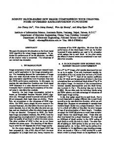
for the RRQR recompression kernels which leads to a better limitation of the rank growth during the factorization. We present a detailed analysis of the solver with a parallelism study and a comparison of efficiency of the low-rank kernels with respect to the original full-rank kernels. We also evaluate the impact of several parameters on the memory consumption and time to solution such as the blocking sizes, the maximum rank accepted for low-rank forms and the different orthogonalization methods. In Section 2, we go over basic aspects of sparse supernodal direct solvers. The two strategies, introduced in PaStiX, are then presented in Section 3, before detailing low-rank kernels in Section 4. Section 5 compares the two BLR strategies with the original approach, that uses only dense blocks, in terms of memory consumption, time-to-solution and numerical behaviour. We also investigate the efficiency of low-rank kernels, as well as the impact of the BLR solver parameters. Section 6 surveys in more detail related works on BLR for dense and/or sparse direct solvers, highlighting the differences with our approach, before discussing how to extend this work to a hierarchical format (H, HSS, HODLR. . .). 2. Background on Sparse Linear Algebra The common approach used by sparse direct solvers is composed of four main steps : 1) ordering of the unknowns, 2) computation of a symbolic block structure, 3) numerical block factorization, and 4) triangular system solves. In the rest of the paper, we consider that all problems have a symmetric pattern given by the pattern of A + At . The purpose of the first step is to minimize the fill-in — zero becoming non-zero — that occurs during the numerical factorization to reduce the number of operations as well as the memory requirements to solve the problem. In order to both reduce fill-in and exhibit parallelism, the nested dissection [25] algorithm is widely used through libraries such as Metis [26] or Scotch [27]. Each set of vertices corresponding to a separator constructed during the nested dissection is called a supernode. From the resulting supernodal partition, the second step predicts the symbolic block structure of the final factorized matrix (L) and the block elimination tree. This block structure is composed of one block of columns (column block) for each supernode of the partition, with a dense diagonal block and several dense off-diagonal blocks, as presented in Figure 1 for a 3D Laplacian.

Figure 1. Symbolic factorization of a 10 × 10 × 10 Laplacian matrix partitioned using Scotch.

The goal is to exhibit large block structures to leverage efficient Level 3 BLAS kernels during the numerical factorization. However, one may notice (cf. Figure 1) that the symbolic structure obtained with a general partitioning tool might be composed of many small off-diagonal blocks contributing to larger blocks. These off-diagonal blocks might be grouped together by adding zero to the structure if the BLAS efficiency gain is worthwhile and if the memory overhead induced by the fill-in is limited. Alternatively, it is also possible to reorder supernode unknowns to group off-diagonal blocks together without additional fill-in. A traveling salesman strategy is implemented in PaStiX [28] and divides by more than two the number of these off-diagonal blocks. Other approaches [12, 21] perform a k-way ordering of supernodes, starting from a reconnected graph of a separator, to order consecutively vertices belonging to a same local part of the separator’s graph. Such reordering technique also allows to reduce ranks of the low-rank blocks as shown in [21]. To introduce more parallelism and data locality, the final structure can then be split into tiles 3


4

as it is now commonly done in dense linear algebra libraries to fit the computational units granularity. These first two steps of direct solvers are preprocessing stages independent from the numerical values. Note that these steps can be computed once to solve multiple problems similar in structure but with different numerical values. Finally, the last two steps, numerical factorization and triangular systems solves, perform the numerical operations. We consider here only the first one for the PaStiX solver. During the numerical factorization, the elimination of each supernode (column block) is similar to standard dense algorithms : 1) factorize the dense diagonal block, xxTRF, 2) solve the off-diagonal blocks belonging to this supernode, TRSM, and 3) apply the updates on the trailing submatrix, GEMM. Those steps are then adapted to the low-rank storage format as explained in Section 3. 3. Block Low-Rank solver In this section, we describe the main contribution of this paper which is a BLR solver developed within the PaStiX library. First we introduce the notation used in this article, and the basics used to integrate low-rank blocks in the solver. Then, using the newly introduced structure, we describe two different strategies leading to a sparse direct solver that optimizes the memory consumption and/or the time-to-solution. In this work, we use the same static pivoting strategy as the full-rank version of the solver and which was first introduced in a sparse direct solver in [29]. 3.1. Notation A k ,(1:b ) k

A k ,( j) ...

A k ,(i) ...

A(0), k

A( j ),k

A (j),( j)

...

A(1: b ), k k

A (j),(i)

A (i),k ...

A (i),(j)

Figure 2. Symbolic block structure and notations used for the algorithms for the column block of index k, and its associated blocks. The larger gray boxes highlight the fact that the contributions modify only a part of the target blocks.

Let us consider the symbolic block structure of a factorized matrix L, obtained through symbolic block factorization. Initially, we allocate this structure initialized with the entries of A and perform an in-place factorization. We denote initial blocks by A and blocks in their final state by L (or U). The matrix is composed of Ncblk column blocks, where each column block is associated with a supernode, or to a subset of unknowns in a supernode when the latter is split to create parallelism. Each column block k is composed of bk + 1 blocks, as presented in Figure 2 where : — A(0),k (= Ak,(0) ) is the dense diagonal block ; — A( j),k is the jth off-diagonal block in the column block with 1 ≤ j ≤ bk , ( j) being a multi-index describing the row interval of each block, and respectively, Ak,( j) is the jth off-diagonal block in the row block ; — A(1:bk ),k represents all the off-diagonal blocks of the column block k, and Ak,(1:bk ) all the off-diagonal blocks of the symmetric row block ; — A(i),( j) is the rectangular dense block corresponding to the rows of the multi-index (i) and to the columns of the multi-index ( j). In addition, we denote Aˆ the compressed representation of a matrix A. 4


5

Full Rank Low Rank

Figure 3. Block Low-Rank compression.

3.2. Sparse direct solver using BLR compression The BLR compression scheme is a flat, non-hierarchical format, unlike others mentioned in the introduction. If we consider the example of a dense matrix, the BLR format clusters the matrix into a set of smaller blocks, as presented in Figure 3. Diagonal blocks are kept dense and off-diagonal blocks are admissible for compression. Thus, these off-diagonal blocks can be represented through a low-rank form uvt , obtained with a compression technique such as Singular Value Decomposition (SVD) or Rank-Revealing QR (RRQR) factorization. Compression techniques are detailed in Section 4. We propose in this paper to apply this scheme to the symbolic block structure of sparse direct solvers. Firstly, diagonal blocks of the largest supernodes in the block elimination tree can be considered as large dense matrices which are compressible with the BLR approach. In fact, as we have seen previously, it is common to split these supernodes into a set of smaller column blocks in order to increase the level of parallelism. Thus, the block structure resulting from this operation gives the cluster of the BLR compression format. Secondly, interaction blocks from two large supernodes are by definition long distance interactions, and thus can be represented by a low-rank form. It is then natural to store them as low-rank blocks as long as they are large enough. To summarize, if we take the final symbolic block structure (after splitting) used by the PaStiX solver, all diagonal blocks are considered dense, and all off-diagonal blocks might be stored using a low-rank structure. In practice, we limit this compression to blocks of a minimal size, and all blocks with relatively high ranks are kept dense. From the original block structure, adapting the solver to block low-rank compression mainly relies on the replacement of the dense operations with the equivalent low-rank operations. Still, different variants of the final algorithm can be obtained by changing when and how the low-rank compression is applied. We introduce two scenarios : Minimal Memory, which compresses the blocks before any other operations, and Just-In-Time which compresses the blocks after they received all their contributions. Algorithm 1 Right looking block sequential LU factorization with Minimal Memory scenario. . /* Initialize A (L structure) compressed */ 1: For k = 1 to Ncblk Do 2: Aˆ (1:bk ),k = Compress( A(1:bk ),k ) 3: Aˆ k,(1:bk ) = Compress( Ak,(1:bk ) ) 4: End For 5: For k = 1 to Ncblk Do 6: Factorize A(0),k = L(0),k Uk,(0) 7: Solve Lˆ (1:bk ),k Uk,(0) = Aˆ (1:bk ),k 8: Solve L(0),k Uˆ k,(1:bk ) = Aˆ k,(1:bk ) 9: For j = 1 to bk Do 10: For i = 1 to bk Do . /* LR to LR updates (extend-add) */ 11: Aˆ (i),( j) = Aˆ (i),( j) − Lˆ (i),k Uˆ k,( j) 12: End For 13: End For 14: End For

5

. LR2LR


6

3.2.1. Minimal Memory This scenario, described by Algorithm 1, starts by compressing the original matrix A block by block without allocating the full matrix as it is done in the full-rank and Just-In-Time strategies. Thus, all low-rank blocks that are large enough are compressed directly from the original sparse form to the low-rank representation (lines 1 − 4). Note that for a matter of conciseness, loops of compression and solve over all off-diagonal blocks are merged into a single operation. In this scenario, compression kernels and later operations could have been performed using a sparse format, such as CSC for instance, until we get some fill-in. However, for the sake of simplicity we use a low-rank form throughout the entire algorithm to rely on blocks and not just on sets of values. Then, each classic dense operation on a low-rank block is replaced by a similar kernel operating on low-rank forms, even for the usual matrix-matrix multiplication (GEMM) kernel that is replaced by the equivalent LR2LR kernel operating on three low-rank matrices (cf. Section 4). Algorithm 2 Right looking block sequential LU factorization with Just-In-Time scenario. 1: For k = 1 to Ncblk Do 2: Factorize A(0),k = L(0),k Uk,(0) . /* Compress L and U off-diagonal blocks */ 3: Aˆ (1:bk ),k = Compress( A(1:bk ),k ) 4: Aˆ k,(1:bk ) = Compress( Ak,(1:bk ) ) 5: Solve Lˆ (1:bk ),k Uk,(0) = Aˆ (1:bk ),k 6: Solve L(0),k Uˆ k,(1:bk ) = Aˆ k,(1:bk ) 7: For j = 1 to bk Do 8: For i = 1 to bk Do . /* LR to dense updates */ 9: A(i),( j) = A(i),( j) − Lˆ (i),k Uˆ k,( j) 10: End For 11: End For 12: End For

. LR2GE

3.2.2. Just-In-Time This second scenario, described by Algorithm 2, delays the compression of each supernode after all contributions have been accumulated. The algorithm is thus really close to the previous one with the only difference being in the update kernel, LR2GE, at line 9, which accumulates contributions on a dense block, and not on a low-rank form. This operation, as we describe in Section 4, is much simpler than the LR2LR kernel, and is faster than a classic GEMM. However, by compressing the initial matrix A, and maintaining the low-rank structure throughout the factorization with the LR2LR kernel, Minimal Memory can reduce more drastically the memory footprint of the solver. Indeed, the full-rank structure of the factorized matrix is never allocated, as opposed to Just-In-Time that requires it to accumulate the contributions. The final matrix is compressed with similar sizes in both scenarios. 3.2.3. Summary For the sake of simplicity, we now compare the three strategies in a dense case to illustrate the potential of different approaches. Figure 4 presents the Directed Acyclic Graph (DAG) of LU operations for the original full-rank version of the solver on a 3-by-3 block matrix. On each node, the couple (i, j) represents respectively the row and column indexes of the block of the matrix being modified. The Minimal Memory strategy generates the DAG described in Figure 5. In this context, the six off-diagonal blocks are compressed at the beginning. In the update process, dense diagonal blocks as well as low-rank off-diagonal blocks are updated. One can notice that off-diagonal blocks are never used in their dense form, leading to memory footprint reduction. However, as we will describe in Section 4, the LR2LR operation in sparse arithmetic is quite expensive and may lead to an increase of time-to-solution. The Just-In-Time strategy generates the DAG described in Figure 6. In this case, the six off-diagonal blocks are compressed throughout the factorization. Since those off-diagonal blocks are used in their dense form before being 6


(1,1)

(2,3)

(1,3)

(2,1)

(1,1)

(3,1)

(1,2)

(3,2)

(3,1)

(1,3)

(1,1)

(1,2)

(2,1)

(1,3)

(2,1)

(3,1)

(1,2)

(1,3)

(2,1)

(3,1)

(1,2)

(3,1)

(1,3)

(1,2)

(2,1)

(2,3)

(3,3)

(2,2)

(3,2)

(2,3)

(3,3)

(2,2)

(3,2)

(3,3)

(3,2)

(2,3)

(2,2)

(2,2)

(3,2)

(2,3)

(2,2)

(3,2)

(3,2)

(2,3)

(2,2)

(2,3)

(3,2)

(2,3)

(3,3)

(3,3)

(3,3)

(3,3)

(3,3)

(3,3)

Figure 4. Full-rank.

Figure 5. Minimal Memory.

7

Compression GETRF TRSM LR2LR GEMM or LR2GE

Figure 6. Just-In-Time.

compressed, there is less room for memory improvement. However, as we will see later, the LR2GE can still be performed efficiently in the sparse case. 4. Low-rank kernels We introduce in this section the low-rank kernels used to replace the dense operations, and we present a complexity study of these kernels. Two families of operations are studied to reveal the rank of a matrix : Singular Value Decomposition (SVD) which leads to smaller ranks, and Rank-Revealing QR (RRQR) which has shorter time-to-solution. 4.1. Compression The goal of low-rank compression is to represent a general dense matrix A of size mA -by-nA by its compressed version Aˆ = uA vtA , where uA , and vA , are respectively matrices of size mA -by-rA , and nA -by-rA , with rA being the rank of the block supposed to be small with respect to mA and nA . In order to keep a given numerical accuracy we have to ˆ ≤ τ||A||, where τ is the prescribed tolerance. choose rA such that ||A − A|| 4.1.1. SVD A is decomposed as UΣV t . The low-rank form of A consists of the first rA singular values and their associated singular vectors such that : ΣrA +1 ≤ τ||A||, uA = UrA , and vtA = Σ1:rA VrtA with UrA (respectively VrA ) being the first rA columns of U (respectively V). This solution presents multiple drawbacks. It has a large cost of Θ(m2A nA + n2A mA + n3A ) operations to compress the matrix, and all singular values needs to be computed to get the first rA ones. On the other hand, as the singular values of the matrix are explicitly computed, it leads to the lowest rank for a given tolerance. 4.1.2. RRQR A is decomposed as QRP, where P is a permutation matrix, and QR the QR decomposition of AP−1 . The low-rank form of A of rank rA is then formed by uA = Q(:,rA ) , the first rA columns of Q, and by vtA = R(rA ,:) , the first rA rows of R. The main advantage of this process is that one can stop the factorization as soon as the norm of the trailing submatrix A˜ (rA +1:mA ,rA +1:nA ) = A − Q(:,rA ) R(rA ,:) P is lower than τ||A||. Thus, the complexity is lowered to Θ(mA nA rA ) operations. However, it returns an evaluation of the rank which might be a little larger than those returned by SVD and generate more flops during the numerical factorization and solve. In conclusion, SVD is much more expensive than RRQR. However, for a given tolerance, SVD returns lower ranks. Put another way, for a given rank, SVD will have better numerical accuracy. Thus, there is a trade-off between time-to-solution (RRQR) versus memory consumption (SVD). 7


8

Note that for the Minimal Memory scenario, the first compression (of sparse blocks) may be realized using Lanczos’s methods, to take advantage of sparsity. However, both SVD and RRQR algorithms inherently take advantage of these zeros. In addition, most of the low-rank compression are applied to blocks stored as dense blocks and represent the main part of the computation. 4.2. Solve The solve operation for a generic lower triangular matrix L is applied to blocks in low-rank forms in our two scenarios : L xˆ = bˆ ⇔ Lu x vtx = ub vtb . Then, with vtx = vtb , the operation is equivalent to applying a dense solve only to ub , and the complexity is only Θ(m2L r x ), instead of Θ(m2L nL ) for the full-rank (dense) representation. 4.3. Update Let us consider the generic update operation, C = C − ABt . Note that the PaStiX solver stores L, and U t if required. Then, the same update is performed for Cholesky and LU factorizations. We break the operation into two steps : the product of two low-rank blocks, and the addition of a low-rank block to either a dense block (LR2GE), or a low-rank block (LR2LR). 4.3.1. Low-rank matrix product This operation can simply be expressed as two dense matrix products : Aˆ Bˆ t = (uA (vtA vB ))utB = uA ((vtA vB )utB ), where uA is kept unchanged if rA ≤ rB (utB is kept otherwise) to lower the complexity. However, it has been shown in [19] that the rank rAB of the product of two low-rank matrices of ranks rA and rB is usually smaller than min(rA , rB ). As uA and uB are both orthogonal, the matrix E = (vtA vB ) has the same rank as Aˆ Bˆ t . Thus, the complexity can be further reduced by transforming the matrix product to the following series of operations : E = vtA vB t t Eˆ = vd A v B = uE vE

(1)

uAB = uA uE

(3)

vtAB = vtE vtB .

(4)

(2)

4.3.2. Low-rank matrix addition Let us consider the next generic operation C 0 = C − uAB vtAB , with mAB ≤ mC and nAB ≤ nC as it generally happens in the supernodal method. This is illustrated for example by the update block A(i),( j) in Figure 2. If C is not compressed, as it happens in the LR2GE kernel, C 0 will be dense too, and the addition of the two matrices is nothing else than a GEMM kernel. The complexity of this operation grows as Θ(mAB nAB rAB ). rC

rAB

0

mC

uC

uAB

0

Figure 7. Accumulation of two low-rank matrices when sizes do not match.

If C is compressed as in the LR2LR kernel, C 0 will be compressed too, and uC 0 vCt 0

Cˆ 0 = uC vCt − uAB vtAB

(5)

= [uC , uAB ]([vC , −vAB ]) 8

(6)

t


9

where [, ] is the concatenation operator. The update given at Equation (5) is the commonly named extend-add operation. Without further optimization, this operation costs only two copies. In the case of the supernodal method, adequate padding is also required to align the vectors coming from the AB and C matrices as shown in Figure 7 for the u vectors. The operation on v is similar. One can notice that in this form, the rank of the updated C is now rC + rAB . When accumulating multiple updates, the rank grows quickly and the storage exceeds the full-rank version. In order to maintain a small rank for C, recompression techniques are used. As for the compression kernel, both SVD and RRQR algorithms can be used. Recompression using SVD. We start by computing a QR decomposition for both composed matrices : [uC , uAB ] = Q1 R1 and [vC , −vAB ] = Q2 R2 .

(7)

Then, the temporary matrix T = R1 Rt2 is compressed using the SVD algorithm described previously. This gives the final Cˆ 0 with : uC 0 = (Q1 uT ) and vC 0 = (Q2 vT ). (8) The complexity of this operation is decomposed as follows : Θ((mC +nC )(rC +rAB )2 ) for the two QR decompositions of equation (7), Θ((rC + rAB )3 ) for the SVD decomposition, and finally Θ((mC + nC )(rC + rAB )rC 0 ) for the application of both Q1 and Q2 . Recompression using RRQR. This solution takes advantage of the fact that uC is orthonormal to first orthogonalize uAB with respect to uC . For this operation, we refer to Section 4.3.3 to form an orthonormal basis [uC , uAB ] such that [uC , uAB ] = [uC , uAB ] T.

(9)

We follow by applying the RRQR algorithm to : t T [vC , −vAB ] = QRP.

(10)

As for the compression, we keep the k = rC 0 first columns of Q and rows of R to form the final C 0 : uC 0 = ([uC , uAB ] Qk ) and vCt 0 = Rk P.

(11)

Note that uC 0 is kept orthonormal for future updates. When the RRQR algorithm is used, the complexity of the recompression is then composed of : Θ(rC rAB mAB ) to form the intermediate product uCt uAB , Θ(mC rC rAB ) to form the orthonormal basis, Θ(nAB rAB rC ) to generate the temporary matrix used in (10), Θ((rC + rAB )nC rC 0 ) to apply the RRQR algorithm, and finally again Θ((rC + rAB )nC rC 0 ) to compute the final uC 0 . 4.3.3. Orthogonalization Let us consider the orthogonalization of [uC , uAB ] = QT , taking advantage of uC orthogonality. The following recompression of T [vC , −vAB ]t will now be referred as right recompression. A main issue is that [uC , uAB ] may not be full-rank in exact arithmetic if both matrices share a common spectrum. Thus, if some zero columns can be removed, it will reduce the cost of the right recompression, by ignoring zero rows. In practice, for each zero column, we permute both [uC , uAB ] and [vC , −vAB ] matrices and reduce the rank involved in next computations. The objective is to reduce the number of operations depending on rC , considering that in many cases rAB < rC as many large off-diagonal blocks receive small contributions. In order to do so, we perform Gram-Schmidt (GS) projections to take advantage of uC orthogonality. Two variants of GS are widely used : Classical Gram-Schmidt (CGS) and Modified Gram-Schmidt (MGS). Both may have stability issues, and several iterations may be performed to ensure a correct (at machine precision) orthogonality. In practice, we use CGS for its locality advantages and perform a second iteration if required. To verify that a second iteration is required, we use a widely used criterion [30] and did not experience any orthogonality issue for the set of problems we consider. We now present several variants for orthogonalization. 9


10

Householder QR factorization. This method performs a Householder QR factorization on the full matrix [uC , uAB ] = Q1 R1 . Thus, it does not exploit the existing orthogonality in uC , and cannot properly extract zero columns from the final solution to reduce the cost of later operations. However, it is probably the most stable approach and is the mostly tuned kernel in linear algebra libraries such as Intel MKL. The complexity of this operation grows as Θ(mC (rC +rAB )2 ). PartialQR. It performs a projection of uAB into uC : t ug AB = uAB − uC (uC uAB ).

(12)

! I uCt uAB [uC , uAB ] = [uC , ug . AB ] 0 I

(13)

From this projection, we obtain :

g In practice, we perform two projections to ensure the stability. We now have uC ⊥ ug AB and want to orthogonalize u AB to obtain an orthogonal basis. In order to do so, we either perform a Householder QR factorization ug AB = uAB R or a rank-revealing QR factorization at the machine precision ug AB = Qk Rk P to remove zero columns. The first approach can make a good use of Level 3 BLAS operations while the second is less efficient but may construct zero columns and then reduce the right recompression. Classical Gram-Schmidt. In this variant, we orthogonalize one-by-one each vector of uAB with one or two CGS iterations depending on the criterion presented before. The orthogonalization of the i-th column of uAB to obtain the corresponding column of uAB is performed with : uABi = uABi − uAB0:i−1 utAB0:i−1 uABi .

(14)

Each column is then removed after its orthogonalization if it is a zero column. This reduces the final rank of the update and the cost of the following operations. In the experimental study, we will compare the three approaches in terms of operation count and performance. For orthogonality, we did not observe any numerical issue in our test problems. Note that for both PartialQR and CGS, only last rAB rows of ([vC , −vAB ])t are updated. For those two methods, the orthogonalization complexity grows as Θ(mC rC rAB ). 4.4. Summary Table 1 presents the computational complexity for the two low-rank strategies with respect to the original version of the solver. The main factor of complexity is computed under the assumption that mC ≥ mA ≥ mB , rA ≥ rB , mC ≥ nC , and rC ≤ rC 0 . It does not depend on nA but on the ranks rA and rB : there are fewer operations to be performed. On the other hand, the Minimal Memory strategy requires using either the SVD or RRQR recompression, for which the complexity depends on mC and nC , the dimensions of the block C. This explains why this strategy appears as a higher complexity than the original solver. When considering dense matrices, the low-rank matrix (blocks) are updated by contributions of the same size. In that case, the complexity of the low-rank update becomes asymptotically cheaper than the full-rank updates, and leads to performance gain. This is exploited in dense BLR solvers as [19], and in the CUFS (Compress, Update, Factor, Solve) strategy of the BLR-MUMPS solver, which compresses a dense front before applying operations between low-rank blocks of the same size. In the supernodal approach, blocks belonging to last level separators receive many small contributions, as illustrated in Figure 1. Thus, rC 0 is often close to or equal to rC and lower than rC + rAB : the rank is often invariant when applying a small contribution, which makes RRQR recompression more efficient than SVD recompression, and especially when an orthogonalization method that reduces the basis on the fly is used. In terms of complexity, it is important to notice that the LR2LR update depends on the size of the target block C, and not on the contribution size as in full-rank. Thus, low-rank contributions between blocks of similar sizes are asymptotically cheaper than full-rank contributions on these blocks. Dense and multifrontal solvers exploit this property as they work only on regular block sizes. At the opposite, small updates to larger blocks, that regularly appear in supernodal solvers, have a higher cost in low-rank than in full-rank. In summary, we can decompose supernodal solvers in two groups of contributions : 10


11

Table 1. Summary of the operation complexities when computing C = C − ABt .

GEMM (Dense)

LR2GE (Just-In-Time) SVD

RRQR

LR2LR (Minimal Memory) SVD

(1) : Θ(nA rA rB ) LR matrix product

−

(2) : Θ(rA2 rB )

(2) : Θ(rA rB rAB )

RRQR (1) : Θ(nA rA rB )

(2) : Θ(rA2 rB )

(3), (4) : Θ(mA rA rAB )

(2) : Θ(rA rB rAB )

(3), (4) : Θ(mA rA rAB ) (7) : Θ(mC (rC + rAB )2 )

LR matrix addition

−

Dense update

Θ(mA mB nA )

Main factor

Θ(mA mB nA )

3

−

Θ(mA mB rAB ) Θ(mA mB rAB )

Θ(mA mB rAB )

(12) : Θ(mC rC rAB )

(SVD) : Θ((rC + rAB ) )

(10) : Θ(nC (rC + rAB )rC 0 )

(8) : Θ(mC (rC + rAB )rC 0 )

(11) : Θ(mC (rC + rAB )rC 0 )

−

−

Θ(mC (rC + rAB )2 )

Θ(mC (rC + rAB )rC 0 )

— the updates that will occur within each supernode at the top of the elimination tree and which are generated by regular split of the supernode to generate parallelism, as well as updates from direct descendants of the sons. These contributions work on regular sizes and will reduce the complexity of the solver as observed in dense and multifrontal solvers ; — the updates from deeper descendants in the elimination tree that generate updates from small blocks to larger nodes of the elimination tree. In these contributions, the complexity is defined by the target block, and thus the cost of the low-rank updates may increase the complexity of the solver with respect to the full-rank solver. The experiments showed that this overhead slows down the solver with the Minimal Memory strategy on small problems, but when the problem size increases this strategy outperforms the full-rank factorization. The main advantage of the Minimal Memory scenario is that it can drastically reduce the memory footprint of the solver, since it compresses the matrix before the factorization. Thus, the structure of the full-rank factorized matrix is never allocated, and the low-rank structure needs to be maintained throughout the factorization process to lower the memory peak. 4.5. Kernel implementation In practice, as we manage both dense and low-rank blocks in our solver, we adapt the extend-add operation for each basic case to be as efficient as possible. The optimizations are designed for the RRQR version, in practice SVD is only used as a reference for the optimal compression rates. One of the important criteria for efficient low-rank kernels is the setup of the maximum rank above which the matrix will be considered as non compressible. The setting of this parameter is strategy and application dependent. In practice for an m-by-n matrix, if the main objective is the memory consumption, as in the Minimal Memory strategy, mn the ranks are limited to m+n to reduce as much as possible the final size of the factors without considering the number of flops that are generated. In contrast, if the objective is to reduce the time-to-solution, then the maximum ranks are defined by min(m,n) for which the low-rank operations remains cheaper in number of operations than the full-rank ones. 4 In practice, it also depends on the ranks of the blocks that will be involved in the update and cannot be computed before compression. For a real-life application, the criterion has to be set depending on the number of factorizations (second criterion is more important) and the number of solves (first criterion will reduce the size of the factors and thus the cost of the solve step). The impact of this parameter is studied in 5.6.3. Eventually, when a low-rank block receives a contribution with a high rank, i.e., (rC + rAB ) ≤ maxrank , the C matrix is decompressed to receive the update and then recompressed, instead of directly adding low-rank matrices. This is denoted as Decompression / Recompression of C in the following section. 11


12

There is also a trade-off between using a strict compression criterion and a smaller one due to the efficiency of lowrank operations with respect to dense operations. In practice, we add another parameter named rank ratio to control the maximum rank authorized during compression as a percentage of the strict theoretical rank. 5. Experiments Experiments were conducted on the Plafrim 1 supercomputer, and more precisely on the miriel cluster. Each node is equipped with two Intel Xeon E5-2680v3 12-cores running at 2.50 GHz and 128 GB of memory. The Intel MKL 2017 is used for BLAS and SVD kernels. The RRQR kernel is issued from the BLR-MUMPS solver [21], and is an extension of the block rank-revealing QR factorization subroutines from LAPACK 3.6.0 (xGEQP3) to stop the factorization when the precision is reached. The PaStiX version used for our experiments is available on the public git repository 2 as the tag 6.0.0. The multi-threaded version used is the static scheduling version presented in [31]. Note that for low-rank strategies, we never perform LLt factorization because compression can destroy the positive-definite property. In the case where the matrix is SPD, we use LDLt factorization for low-rank strategies. For the initial ordering step, we used Scotch [27] 6.0.4 with the configurable strategy string from PaStiX to set the minimal size of non-separated subgraphs, cmin, to 15. We also set the f rat parameter to 0.08, meaning that column aggregation is allowed by Scotch as long as the fill-in introduced does not exceed 8% of the original matrix. In experiments, blocks that are larger than 256 are split into blocks of size within the range 128−256 to create more parallelism while keeping sizes large enough. The same 128 criteria is used to define the minimal width of the column blocks that are compressible. An additional limit on the minimal height to compress an off-diagonal block is set to 20. We set the rank ratio to 1 to illustrate the results when the rank is as strict as possible to obtain Flops and/or memory gains. CGS orthogonalization is also used. Note that in Section 5.6 we try different blocking sizes to experiment the impact on the solver, relax the maximum ranks authorized, and compare the orthogonalization strategies. Experiments were computed on a set of 3D matrices from The SuiteSparse Matrix Collection [32], described in Table 2. Table 2. Real-life matrices used in experiments.

Matrix

Precision

Method

Size

Field

Ops (TFlops)

Memory (GB)

Atmosmodj Audi Hook Serena Geo1438

d d d d d

LU LLt LDLt LDLt LLt

1 270 432 943 695 1 498 023 1 391 349 1 437 960

atmospheric model structural problem model of a steel hook gas reservoir simulation geomechanical model of earth

12.1 5.5 8.6 28.6 18.0

16.3 9.5 12.7 21.7 20.1

We also used 3D Laplacian generators (7 point stencils), and defined lap120 as a Laplacian of size 1203 . 2 Note that when results showing numerical precision are presented, we used the backward error on b : ||Ax−b|| ||b||2 . 5.1. SVD versus RRQR The first experiment studies the behaviour of the two compression methods coupled with both Minimal Memory and Just-In-Time scenarios on the matrix Atmosmodj. Table 3 presents the sequential timings of each operation of the numerical factorization with a tolerance of 10−8 , as well as the memory used to store the final coefficients of the factorized matrix. 1. https://www.plafrim.fr 2. https://gitlab.inria.fr/solverstack/pastix

12


13

Table 3. Cost distribution on the Atmosmodj matrix with τ = 10−8 .

Full-rank Factorization time (s) Compression Block factorization (GETRF) Panel solve (TRSM) Update Formation of contribution Addition of contribution Dense udpate (GEMM) Total Solve time (s) Factor final size (GB) Memory peak for the factors (GB)

Just-In-Time SVD RRQR

Minimal Memory SVD RRQR

7.2e-01 1.7e+01

4.1e+02 7.4e-01 6.9e+00

3.4e+01 7.3e-01 7.4e+00

1.8e+02 7.8e-01 7.6e+00

5.6+00 7.6e-01 7.9e+00

4.6e+02 4.7e+02 6.3e+00 16.3 16.3

1.3e+02 5.5e+02 1.9e+00 6.95 16.3

9.7e+01 1.4e+02 3.0e+00 7.49 16.3

9.9e+01 3.0e+03 2.8e+01 3.6e+03 1.5e+00 6.85 6.85

4.2e+01 7.3e+02 2.4e+01 8.1e+02 3.2e+00 7.31 7.31

We can first notice that SVD compression kernels are much more time consuming than the RRQR kernels in both scenarios following the complexity study from Section 4. Indeed, RRQR compression kernels stop the computations as soon as the rank is found which reduces by a large factor the complexity, and this reduction is reflected in the time-to-solution. However, the SVD allows, for a given tolerance, to get better memory reduction in both scenarios. Comparing the Minimal Memory and the Just-In-Time scenario, the compression time is minimized in the Minimal Memory scenario because the compression occurs on the initial blocks which hold more zero and are lower rank than when they have been updated. The time for the update addition, extend-add operation, becomes dominant in the Minimal Memory scenario, and even explodes when SVD is used. This is expected as the complexity depends on the largest blocks in the addition even for small contributions (see Section 4). Note that this ratio will evolve in favor of the extend-add operation on larger matrices where the ratio of updates of same size becomes dominant with respect to the number of updates from small blocks. For both compression methods, both scenarios compress the final coefficients with similar rates. The diagonal block factorization time is invariant in the five strategies : the block sizes and kernels are identical. Panel solve, update product, and solve times are reduced in all low-rank configurations compared to the dense factorization and the timings follow the final size of the factors, since this size reflects the final ranks of the blocks. To conclude, the Minimal Memory scenario is not always able to compete with the original direct factorization on these test cases due to the costly update addition. However, it reduces the memory peak of the solver to the final size of the factors. The Minimal Memory/RRQR offers a 50% memory reduction while doubling the sequential time-to-solution. The Just-In-Time scenario competes with the original direct factorization, and divides by three the time-to-solution with RRQR kernels. 5.2. Performance Figure 8 presents the overall performance achieved by the two low-rank scenarios with respect to the original version of the solver (where lower is better) on the previously introduced set of six matrices. All versions are multithreaded implementations and use the 24 cores of one node. The scheduling used is the PaStiX static scheduler developed for the original version, this might have a negative impact for low-rank strategies by creating a load imbalance. We study only the RRQR kernels as the SVD kernels have shown to be much slower. Three tolerance thresholds are studied for their impact on the time-to-solution and the accuracy of the backward error. The backward errors printed on top of each bar correspond to the use of one refinement step. 13


audi

Geo1438

lap120

(a) Just-In-Time scenario using RRQR.

atmosmodj

audi

Geo1438

4.4e-07 2.4e-11 3.8e-04

2.1e-07 4.5e-11

τ =10−12 1.7e-04 1.3e-07 2.4e-12

τ =10−8

5.9e-04

Serena

1.8e-08 7.1e-13

9.1e-13

Hook

0.2 0.0

τ =10−4

9.3e-04 4.8e-06 4.3e-11

atmosmodj

5.7e-05 1.9e-08 1.8e-12

0.6 0.4

4.2e-04 3.7e-10 7.4e-15

1.1e-05 6.5e-10 1.6e-14

lap120

0.8

6.9e-05 1.4e-08

1.2 1.0

2.6e-04 2.4e-10 2.1e-15

1.4

4.5 4.0 3.5 3.0 2.5 2.0 1.5 1.0 0.5 0.0

8.7e-05

τ =10−12

7.0e-05 4.0e-08 8.9e-13

τ =10−8

Time BLR / Time PaStiX

τ =10−4

1.0e-05 6.1e-10 2.3e-14

Time BLR / Time PaStiX

1.6

14

Hook

Serena

(b) Minimal Memory scenario using RRQR.

Figure 8. Performance of both low-rank strategies with three tolerance thresholds. The backward error of the solution is printed on top of each bar.

Figure 8(a) shows that the Just-In-Time/RRQR scenario is able to reduce the time-to-solution in almost all cases of tolerance, and for all matrices which have a large spectrum of numerical properties. These results show that applications which require low accuracy, as the seismic application for instance, can benefit by up to a factor of 3.5. Figure 8(b) shows that it is more difficult for the Minimal Memory/RRQR scenario to be competitive. The performance is often degraded with respect to the original PaStiX performance, with an average loss of around a factor 2, and the tolerance has a much lower impact than for the previous case. For both scenarios, the backward error of the first solution is close to the entry tolerance. It is a little less accurate in the Minimal Memory scenario, because approximations are made earlier in the computation, and information is lost from the beginning. However, these results show that we are able to catch algebraically the information and forward it throughout the update process. 5.3. Memory consumption 1.4

2.4e-11 2.9e-11

4.4e-07 4.2e-07 3.8e-04 4.0e-04

1.3e-07 1.2e-07 2.4e-12 1.8e-12

RRQR, τ =10−12 SVD, τ =10−12

1.7e-04 1.8e-04

4.5e-11 3.1e-11

2.1e-07 2.5e-07 5.9e-04 6.5e-04

0.4

9.3e-04 1.3e-03

0.6

8.7e-05 7.4e-05 1.8e-08 7.2e-09 7.1e-13 4.2e-13

0.8 7.0e-05 5.5e-05 4.0e-08 1.0e-08 8.9e-13 4.1e-13

Memory BLR / Memory PaStiX

1.0

RRQR, τ =10−8 SVD, τ =10−8 4.8e-06 4.6e-06 4.3e-11 2.8e-11

RRQR, τ =10−4 SVD, τ =10−4

1.2

0.2 0.0

lap120

atmosmodj

audi

Geo1438

Hook

Serena

Figure 9. Memory peak for the Minimal Memory scenario with three tolerance thresholds and both SVD and RRQR kernels. The backward error of the solution is printed on top of each bar.

The Minimal Memory scenario is slower than the original solver in most cases, but it is a strategy that efficiently reduces the memory peak of the solver. Figure 9 presents the gain in the memory used to store the factors at the end of the factorization of the set of six matrices with respect to the block dense storage of PaStiX. In this figure, we also compare the memory gain of the SVD and RRQR kernels. We observe that in all cases, SVD provides better compression rate by finding smaller ranks for a given matrix and a given tolerance. The quality of the backward error is in general slightly better with the SVD kernels despite the smaller ranks. The second observation is that the 14


15

smaller the tolerance (10−12 ), the larger the ranks and the memory consumption. However, the solver always presents a memory gain larger than 50% with larger tolerance (10−4 ). Figure 10(a) presents the evolution of the size of the factors as well as the full consumption of the solver (factors and management structures) on 3D Laplacians with an increasing size. The memory limit of the system is 128GB. The original version is limited on this system to a 3D Laplacian of 8 million unknowns, and the size of the factors quickly increases for larger number of unknowns. With the Minimal Memory/RRQR scenario, we have now been able to run a 3D problem on up to 36 million unknowns when relaxing the tolerance to 10−4 . From the same experiment, Figure 10(b) presents the number of operations evolution depending on the Laplacians size. One can note that for a small number of unknowns, Minimal Memory/RRQR scenario performs more operations than the original, full-rank, factorization. However, for a large number of unknowns, the number of operations is reduced by a large factor. For instance, for a 2803 Laplacian with a 10−8 tolerance, the number of operations is reduced by a factor larger than 36. It demonstrates the potential of our approach : even if operations are less efficient and may lead to a time-to-solution overhead for relatively small problems, the Minimal Memory strategy enables the computation of larger problem and reduces its time-to-solution. In this experiment, the Minimal Memory strategy becomes faster for Laplacian larger than 1503 with a 10−8 tolerance. 103

1016 1015

102

10-1 10-2

Full-rank τ =10−12 τ =10−8 τ =10−4

10-3

1012 1011 1010 109

Full-rank τ =10−12 τ =10−8 τ =10−4

108 107

Size

(a) Memory.

110 3 130 3 150 3 170 3 190 3 210 3 230 3 250 3 270 3 290 3 310 3 330 3

106

110 3 130 3 150 3 170 3 190 3 210 3 230 3 250 3 270 3 290 3 310 3 330 3

10 3 30 3 50 3 70 3 90 3

10-4

Number of operations

100

1013

10 3 30 3 50 3 70 3 90 3

Size of the factors (GB)

1014

101

Size

(b) Number of operations.

Figure 10. Scalability of the memory on top and the number of operations on bottom with three tolerance thresholds of the Minimal Memory/RRQR scenario for 3D Laplacians of size n3 with n ∈ [10, 330]. The full-rank scenario, in purple, is given as a reference with the numbers computed from the symbolic factorization.

The memory of the Just-In-Time scenario has not been studied, because in our supernodal approach, each supernode is fully allocated in a full-rank fashion in order to accumulate the updates before being compressed. Thus, the memory peak corresponds to the totality of the factorized matrix structure without compression and is identical to the original version. To reduce this memory peak, a solution would be to modify the scheduler to a Left-Looking approach that would delay the allocation and the compression of the original blocks. However, it would need to be carefully implemented to keep a certain amount of parallelism in order to save both time and memory. A possible solution is the scheduling strategy presented in [33] to keep the memory consumption of the solver under a given limit. 5.4. Convergence and numerical stability Figure 11 presents the convergence of the GMRES iterative solver preconditioned with the low-rank factorization at tolerances of 10−4 and 10−8 . The iterative solver is stopped after reaching 20 iterations or a backward error lower than 10−12 . With a tolerance of 10−8 , only a few iterations are required to converge to the solution. Note that on the Audi and Geo1438 matrices, which are difficult to compress, a few more iterations are required to converge. With a larger tolerance 10−4 , it is difficult to recover all the information lost during the compression, but this is enough to quickly get solutions at 10−6 or 10−8 . Note that the GMRES process benefits from the compression, as the solve step. 15


16

10-2 10-3 10-4

τ =10−4

10-5 Backward error: ||Ax||b−||2b||2

10-6

audi Geo1438 Hook Serena lap120 atmosmodj

10-7 10-8 10-9 10-10

τ =10−8

10-11 10-12 10-13 10-14

0

5

10 Number of GMRES iterations

15

20

Figure 11. Convergence speed for the Minimal Memory/RRQR scenario with two tolerance thresholds.

5.5. Parallelism For the full-rank factorization, supernodes are split between processors depending on the corresponding number of operations. When a target block C receives a contribution, a lock is used to ensure that the block is not modified simultaneously by several threads. For the Just-In-Time strategy, a similar lock is used since the update operations directly apply dense modifications. However, for the Minimal Memory strategy, the update operation is decomposed into two parts : Formation of contribution and Addition of contribution. Because the formation of contribution does not depend on the target block C, the lock is only positioned for the addition of contribution, which may increase the level of parallelism. Figure 12 presents the speedup of the full-rank factorization and low-rank strategies using tolerances of 10−4 and −8 10 for the atmosmodj matrix. The speedup for the full-rank version is above 12, for a relatively small matrix. The speedup of the Minimal Memory strategy is above 11, while the speedup of the Just-In-Time strategy is around 8. As the supernodes distribution cannot predict the ranks and the corresponding number of operations, load balancing may be degraded. Minimal Memory strategy scalability exceeds Just-In-Time strategy because there are less constraints on locks. Note that on recent architectures, the maximal speedup can not be obtained, as the CPU frequency is reduced when all cores are used on the node, while it is increased for single core operation. We thus computed an approximate maximum speedup of 20.7 on this architecture for the Intel MKL BLAS GEMM operation. 5.6. Kernels analysis In this section, we focus on the atmosmodj matrix to illustrate the performance of basic kernels as well as the impact of several parameters. As in practical cases we use RRQR instead of SVD, we will focus on this compression kernel for each strategy. 5.6.1. Performance of basic kernels We evaluate the performance rate (in GFlops/s) for the full-rank factorization and for the two low-rank strategies, and use a 10−8 tolerance. Figure 13(a) (respectively Figure 13(b)) presents the runtime distribution among kernels for the full-rank (respectively Just-In-Time) factorization. We can note that in both cases, the Update process is the most time-consuming. For the Just-In-Time strategy, Compression and TRSM are not negligible, because the Update runtime is much reduced with respect to full-rank factorization. Figure 13(c) presents the runtime distribution among kernels for the Minimal Memory strategy with three different levels from the left to the right : the main steps of the solver, the details for the Update kernels, and the details for 16


16

Full-rank Minimal-Memory/τ =10−8 Minimal-Memory/τ =10−4 Just-In-Time/τ =10−8 Just-In-Time/τ =10−4

14 12 Speedup

17

10 8 6 4 2 0

2

4

6

8

10 12 14 16 Number of threads

18

20

22

24

Figure 12. Speedup of the factorization for the atmosmodj matrix with 1 to 24 threads.

Compression TRSM GETRF

TRSM

Update Update (a) Full-rank strategy.

(b) Just-In-Time strategy.

Orthogonalization xx2lr

Formation of contribution

Recompression of C+AB

TRSM

Update of the basis Update xx2fr Update dense

General

Details of update

Decompression/ Recompression of C

Details of xx2lr

(c) Minimal Memory strategy. Figure 13. Breakdown of the most time-consuming kernels for the full-rank strategy (top-left), the Just-In-Time strategy (top-right), and the Minimal Memory strategy (bottom) on the atmosmodj case using the RRQR kernels with τ = 10−8 . The analysis of the Minimal Memory strategy is shown at three different levels from the left to the right : the global operations, the partition of the updates between low-rank and full-rank, and the details of the low-rank updates.

17


18

the low-rank updates. Note that xx2fr refers to a full-rank update within a compressible supernode (i.e., an update to a dense block which was originally considered compressible) while xx2lr is a low-rank update, xx being one of the four possible matrix products : low-rank/low-rank, low-rank/full-rank, full-rank/low-rank or full-rank/full-rank. Update dense corresponds to blocks that were not considered compressible and managed in dense arithmetic throughout all operations ; as expected the underlying operations represent a small time of computation. We observe that the low-rank update is the most time consuming part. In practice, the Formation of contribution (cf. Section 4.3.1) is quite cheap, while applying the update is expensive ; as we have seen in Table 1, it depends on the size and the rank of the target C. This update addition is decomposed into three main operations : Orthogonalization of the [uC , uAB ] matrix (cf. Section 4.3.3), Recompression of C + AB (cf. Eq (2)) and Update of the basis (cf. Eq (11)). If the contribution rank is too high to take advantage of recompression, we perform a Decompression / Recompression of C (cf. Section 4.5). Table 4 presents the performance of most time-consuming kernels for each type of factorization on a machine where around 32 GFlops/s can be raised for each CPU core when all cores are used. One can note that the performance of kernels for the full-rank factorization is close to the machine peak : the original solver makes good use of Level 3 BLAS even if there are many small blocks. On the other hand, low-rank kernels performing Level 3 BLAS kernels, i.e., Formation of contribution, Update of the basis, TRSM, are running at 31 of the peak. It is due to lower granularity generated by the smaller blocks, which reduce the arithmetic intensity of the kernels. For Compression and Recompression of C+AB kernels, the efficiency is even worse due to the behaviour of RRQR. Table 4. Kernels efficiency per core for full-rank, Just-In-Time and Minimal Memory strategies, on atmosmodj with τ = 10−8 .

Strategy

Name

-

GETRF TRSM Update Compression TRSM Update TRSM Update dense xx2fr xx2lr Formation of contribution Orthogonalization Recompression of C + AB Update of the basis Decompression / Recompression of C

Full-rank

Just-In-Time

Minimal Memory

Nb calls

Time (s)

GFlops

Perf (GFlops/s)

74665 1572464 10993468 44544 1572464 10993468 1572464

981.6 17862.0 446003.1 32831.8 9312.8 126681.3 7355.9

6.4 421.2 12869.6 146.6 111.1 1464.1 103.8

6.5 23.6 28.9 4.5 11.9 11.6 14.1

5782698 2207642

4838.5 31280.6

24.6 285.0

5.1 9.1

3036024 2688031 2499058 2499058 556650

39319.2 115957.9 301204.3 54132.7 256821.7

493.7 630.2 755.4 742.5 2236.3

12.6 5.4 2.5 13.7 8.7

In our implementation, RRQR is a modification of LAPACK xgeqp3 and xlaqps routines. Some stability issues presented in [34] prevent to make efficient use of Level 3 BLAS kernels. To summarize, low-rank strategies are useful to reduce the overall number of operations. However, due to the poor efficiency of low-rank kernels, the gain in flops does not directly translate into timing reduction. One can expect that for larger problems, the reduction in flops will more easily translate into time-to-solution reduction. 5.6.2. Impact of blocking parameters In previous experiments, we always used a splitting criterion of 256 with a minimal size of 128 : blocks larger than 256 are split into a subset of blocks larger than 128. For low-rank strategies, we consider only blocks larger than 128 18


19

as compressible. In Table 5, we evaluate the impact of using different blocking sizes (between 128 and 256 or between 256 and 512) for the full-rank factorization and for three different tolerances using Minimal Memory and Just-In-Time strategies. The minimum width of compressible supernodes is set to the minimum blocksize : either 128 or 256. All results are performed using 24 threads on the atmosmodj matrix. Table 5. Impact of the blocking size parameter on the number of operations, the factorization time, and the memory for the atmosmodj on the Full-rank strategy (top) and on both Minimal Memory and Just-In-Time strategies (bottom). Both low-rank strategies are using RRQR kernels. (a) Full-rank strategy.

Blocksize Full-rank

128–256

256–512

12.1 39.5 16.3

12.1 51.5 16.5

Operations (TFlops) Fact. time (s) Memory (GB)

(b) Low-rank strategies.

Precision Blocksize Minimal Memory

Just-In-Time

Operations (TFlops) Fact. time (s) Memory (GB) Operations (TFlops) Fact. time (s) Memory (GB)

τ = 10−4 128–256 256–512 3.9 76.4 5.8 0.7 10.0 6.0

1.8 49.7 4.7 0.5 12.0 4.9

τ = 10−8 128–256 256–512 4.8 100.1 6.53 0.8 15.6 6.71

10.8 166.6 7.29 1.1 14.4 7.47

τ = 10−12 128–256 256–512 8.3 147.7 8.31 1.3 20.5 8.43

18.0 253.0 8.81 1.5 20.2 8.93

The first observation concerns the full-rank factorization. The blocking sizes impact both the granularity and the level of parallelism. For a sequential run, it is suitable to use large blocking sizes to increase granularity and thus the efficiency of Level 3 BLAS operations. On the other hand, it may degrade parallel performance if there are many workers and not enough supernodes. For the Minimal Memory strategy, we have seen in Table 1 that the number of operations depends on the target size and rank and thus increases a lot with the blocking size. This is true even in the case where ranks are not that much impacted by the blocking size. In practice, we observe that for each tolerance, increasing blocking size degrades factorization time. In addition, as less data is considered as compressible, the size of the factors is growing and this will increase the solve cost. For the Just-In-Time strategy, the impact of blocking size will mostly depend on ranks. If ranks are small, using larger blocks will increase the performance of RRQR and thus reduce the time-to-solution. However if ranks are higher, it will reduce the level of parallelism as in the full-rank factorization. We always observe a gain using a larger blocking size, but the ratio between the use of 256/512 versus 128/256 is decreasing when the tolerance is lower : the granularity gain causes some parallelism issues. 5.6.3. Impact of rank ratio parameter In previous experiments, we use strict maximum ranks, i.e., the limit ranks to reduce the number of flops or the mn memory consumption : m+n for Minimal Memory strategy and min(m,n) for Just-In-Time strategy. In practice, we have 4 seen that for both strategies, kernel efficiency is poor with respect to classical Level 3 BLAS operations. In Table 6 we evaluate the impact of relaxing the constraint on a strict rank for the Minimal Memory and the Just-In-Time strategies. The ratio parameter corresponds to a percentage of the strict maximum rank (used to obtain smaller ranks) and avoid the overhead of managing low-rank blocks with a high rank by turning back these blocks into full-rank form. All results are performed using 24 threads on the atmosmodj matrix. For the Minimal Memory strategy, there are two main observations. Firstly, considering that the update complexity depends on the size but also on the rank of the target C, the burden on recompression of high-rank blocks is reduced, 19


20

Table 6. Impact of the maximum rank ratio on the number of operations, the factorization time, and the memory for the atmosmodj case with RRQR kernels for both Minimal Memory and Just-In-Time strategies.

τ = 10−4 1 0.5 0.25

Precision Ratio Minimal Memory

Just-In-Time

Operations (TFlops) Fact. time (s) Memory (GB) Operations (TFlops) Fact. time (s) Memory (GB)

1.8 48.7 4.7 0.5 11.9 4.9

1.9 49.7 4.7 0.6 11.6 5.0

2.3 43.7 5.4 0.9 10.9 5.9

τ = 10−8 1 0.5 0.25 4.8 100.0 6.53 0.8 14.2 6.71

4.8 85.4 7.0 1.4 15.4 7.23

4.5 56.0 8.94 2.6 17.8 9.12

1 8.3 146.0 8.31 1.3 19.0 8.43

τ = 10−12 0.5 0.25 7.2 105.1 9.26 2.8 20.8 9.36

7.4 65.6 11.71 5.1 25.3 11.73

and sometimes even the number of operations. Secondly, managing more blocks in full-rank fashion can reduce timeto-solution due to the poor efficiency of low-rank kernels. In practice, we observe that using a relaxed criterion always reduces time-to-solution while having only a little impact on the memory. For the Just-In-Time strategy, the maximum rank criterion cannot be set theoretically, because it depends on all ranks within a same supernode. However, contrary to the Minimal Memory approach, the number of operations being really reduced with respect to full-rank factorization, there is a time-to-solution gain and it seems suitable to compress as many blocks as possible. In practice, relaxing the max-rank criteria is only interesting for 10−4 tolerance, for which the granularity is really small. Note that in both cases, relaxing the burden on large ranks increases the size of the factors, and in the same way the cost of the solve. Thus, selecting a suitable criteria will depend on the application and the ratio between the number of factorizations and the number of solves. 5.6.4. Orthogonalization cost In previous Minimal Memory experiments, we used CGS as orthogonalization process. As presented in Section 4.3.3, some other approaches can be investigated. In Table 7, we present the impact of using CGS, Householder QR or PartialQR on the number of operations as well as on the efficiency of the solver. It only impacts intermediate ranks and not the final size of the factors. Table 7. Impact of the orthogonalization method on the number of operations and the factorization time for Minimal Memory strategy on atmosmodj.

Precision Orth. Method Operations (TFlops) Fact. time (s)

CGS 1.8 50.5

τ = 10−4 QR PartialQR 2.8 2.0 60.3 48.5

CGS 4.8 99.1

τ = 10−8 QR PartialQR 8.0 5.1 128.9 96.3

CGS 8.3 145.2

τ = 10−12 QR PartialQR 13.2 8.7 191.8 138.6

As predicted by its complexity, Householder QR factorization is more expensive than both CGS and PartialQR. The difference between CGS and PartialQR is related to the number of columns of zero. While CGS can remove those columns during computations, PartialQR can only deal with those zero after all operations : the number of operations increases for each tolerance. However, in terms of time, PartialQR outperforms CGS especially for small tolerances (10−12 ) due to the efficiency of Level 3 BLAS operations. One can expect that for a larger tolerance (10−4 ), CGS may be faster than PartialQR, because the smaller granularity will degrade the assets of Level 3 BLAS operations.

20


21

6. Discussion In this section, we discuss the positioning of our low-rank strategies with the closest related works and we give some perspectives in extending this work to a hierarchical format. Sparse H solver. In [2], different approaches using H-matrices are summarized, including the extension to the sparse case. The authors use a nested dissection ordering as in our solver, and thus there is no fill-in between distinct branches of the elimination tree. However, contributions of a supernode to its ancestors are considered as full, in the sense that all structural zero are included to generate the low-rank representation. Thus, they do not have extend-add (LR2LR) operations between low-rank blocks of different sizes : assembly is performed as in our Minimal Memory scenario, but without zero padding. The memory consumption is higher with their approach because some structural zeros are not managed : unlike them, we perform a block symbolic factorization to consider sparsity in all contributions between supernodes. Dense BLR solver. A dense BLR solver was designed by Livermore Software Technology Corporation (LSTC) [19]. In this work, the full matrix is compressed at the beginning and operations between low-rank blocks are performed. This approach performs low-rank assembly as in our Minimal Memory scenario. As it handles dense matrices, the extend-add process is performed between low-rank matrices of the same size and zero padding is not required. Thus, the LR2LR operation is less costly than the full-rank update in this context. Sparse Multifrontal BLR solver. A BLR multifrontal sparse direct solver was designed for the Mumps solver. The different strategies are summarized in [22] and a theoretical study of the complexity of the solver for regular meshes is presented in [35]. In the current implementation, the fronts are always assembled in a full-rank form before being compressed. The authors suggest as an alternative solution to assemble the fronts panel by panel to avoid allocating the full front in a dense fashion, but this was not implemented and it will impact the potential parallelism. Mumps is a multifrontal solver, and BLR is considered when eliminating a dense front and not between fronts while our supernodal approach has a more global view of all supernodes. Our scenario Just-In-Time is similar to the FCSU (Factor, Compress, Solve, Update) strategy from [22] where the fronts are compressed panel by panel during their factorization and where only full-rank blocks are updated (LR2GE kernel). The LUAR (Low-Rank Update Accumulation with Recompression) groups together multiple lowrank products to exploit the memory locality during the product recompression process. This could be similarly used in the Just-In-Time strategy, but would imply larger ranks in the extend-add operations of the Minimal Memory strategy. The CUFS (Compress, Update, Factor, Solve) [22] strategy is the closest to the Minimal Memory scenario, as it performs low-rank assembly (LR2LR kernel) within a front. However, the fronts are still first allocated in full-rank to assemble the contributions from the children. Within a front, the CUFS strategy is similar to what was proposed by LSTC for dense matrices. In that case, since blocks are dense and low-rank operations are performed between blocks of equal sizes, zeros padding is not necessary as in the Minimal Memory strategy. We believe that there is more room for memory savings using the Minimal Memory strategy for two reasons : 1) we avoid the extra cost of fronts inherent to the multifrontal method and 2) the low-rank assembly avoids forming dense blocks before compressing them. We demonstrated that the Minimal Memory strategy reduces the number of operations performed on 3D Laplacians and other matrices coming from various applications, which is the main contribution of this paper. A theoretical complexity study has to be performed to investigate if such an approach performs asymptotically the same number of operations as Just-In-Time or Mumps strategies with a constant factor overhead. Low-rank assembly without randomization techniques has only been studied in [10] for 2D problems with the knowledge of the underlying problem, and computing the complexity bounds for a more general case is still an open research problem, we are currently investigating. Extension to hierarchical formats. With the aim of extending our solver to hierarchical compression schemes, such as H, HSS, or HODLR, we consider graphs coming from real-life simulations of 3D physical problems. From a theoretical point of view, the majority of these graphs have a bounded degree or are bounded density graphs [36], and thus good separators [37] can be built. For a n-vertices mesh, time complexity of a direct solver is in Θ(n2 ), and we 4 expect to build a low-rank solver requiring Θ(n 3 ) operations. For memory requirements, the direct approach leads to 4 an overall storage of Θ(n 3 ), while we target a Θ(n log(n)) complexity. 21


22

2

Let us consider the last separator of size Θ(n 3 ) for a 3D mesh, and one of the largest low-rank blocks of this separator in a hierarchical clustering. They have asymptotically the same size. Previous studies have shown that such 1 a block may have a rank of order Θ(n 3 ). For the Just-In-Time scenario, maintaining such a block in a dense form before 4 compressing it requires Θ(n 3 ) memory. Thus, we will still have the same memory peak, but we might encounter a large overhead when compressing off-diagonal blocks with current RRQR and SVD kernels. For the Minimal Memory scenario, we have seen that the cost of the solver can be split in two stages. The low-level one from the elimination tree that generates small updates to large contribution blocks and that might become more expensive with the hierarchical compression, and the high-level where blocks fit the hierarchical structure and generate flops savings. To overcome the issue of the low-level contributions, new ordering techniques need to be investigated to minimize the number of updates on larger off-diagonal blocks. We will also investigate the use of randomization techniques to lower the complexity of the updates from the bottom of the elimination tree. Conclusion We presented a new Block Low-Rank sparse solver that combines an existing sparse supernodal direct solver PaStiX and low-rank compression kernels. This solver reduces the memory consumption and/or the time-to-solution depending on the scenario. Two scenarios were developed. For the set of real-life problems studied, Minimal Memory saves memory up to a factor of 4 using RRQR kernels, with a time overhead that is limited to 2.8. Large problems that could not fit into memory when the original solver was used can now be solved thanks to the lower memory requirements, especially when low accuracy solutions. For larger problems, one can expect that the reduction of the number of operations will translate into a time-to-solution reduction. We experienced this behaviour with large Laplacians : we are now able to solve a 3303 unknowns Laplacian while the original solver was limited to a 2003 unknowns Laplacian, the time-to-solution being reduced over 1503 unknowns. Just-In-Time reduces both the time-to-solution by a factor up to 3.5 and the memory requirements of the final factorized matrix with similar factors to Minimal Memory. However, with the current scheduling strategy, this gain is not reflected in the memory peak. Two compression kernels, SVD and RRQR, were studied and compared. We have shown that, for a given tolerance, both approaches provide correct solutions with the expected accuracy, and that RRQR, despite larger ranks, provides faster kernels. In addition, we demonstrated that the solver can be used either as a low-tolerance direct solver or as a good preconditioner for iterative methods, that normally require only a few iterations before reaching the machine precision. A comparison with other preconditioners (AMG, ILU(k)) will be performed in future work to measure the impact of using a low-rank factorization as a preconditioner. In the future, new kernel families, such as RRQR with randomization techniques, will be studied in terms of accuracy and stability in the context of a supernodal solver. To further improve the performance of Minimal Memory and close up the gap with the original solver, aggregation techniques on small contributions will also be studied. This will lead to the extension of this work to hierarchical compression in large supernodes that could further reduce the memory footprint and the solver complexity. Regarding Just-In-Time, future work is focused on studying smart scheduling strategies that combine RightLooking and Left-Looking approaches in order to find a good compromise between memory and parallelism for the target architecture. Sergent et al. [38] studied scheduling with memory constraints for dense factorization using BLR, and we expect it can be adapted for sparse direct solvers. This will follow up recent work on applying parallel runtime systems [31] to the PaStiX solver. Acknowledgments This material is based upon work supported by the DGA under a DGA/Inria grant. Experiments presented in this paper were carried out using the PlaFRIM experimental testbed, supported by Inria, CNRS (LABRI and IMB), Université de Bordeaux, Bordeaux INP and Conseil Régional d’Aquitaine (see https ://www.plafrim.fr/).

22


23

Références [1] W. Hackbusch, A Sparse Matrix Arithmetic Based on H-Matrices. Part I : Introduction to H-Matrices, Computing 62 (2) (1999) 89–108. [2] W. Hackbusch, Hierarchical Matrices : Algorithms and Analysis, Vol. 49, Springer Series in Computational Mathematics, 2015. [3] L. Grasedyck, R. Kriemann, S. Le Borne, Parallel black box H-LU preconditioning for elliptic boundary value problems, Computing and Visualization in Science 11 (4-6) (2008) 273–291. [4] L. Grasedyck, W. Hackbusch, R. Kriemann, Performance of H-LU preconditioning for sparse matrices, Computational methods in applied mathematics 8 (4) (2008) 336–349. [5] R. Kriemann, H-LU factorization on many-core systems, Computing and Visualization in Science 16 (3) (2013) 105–117. [6] B. Lizé, Résolution directe rapide pour les éléments finis de frontière en électromagnétisme et acoustique : H-matrices. parallélisme et applications industrielles., Ph.D. thesis, École Doctorale Galilée (Jun. 2014). [7] A. Aminfar, S. Ambikasaran, E. Darve, A fast block low-rank dense solver with applications to finite-element matrices, Journal of Computational Physics 304 (2016) 170–188. [8] A. Aminfar, E. Darve, A fast, memory efficient and robust sparse preconditioner based on a multifrontal approach with applications to finite-element matrices, International Journal for Numerical Methods in Engineering 107 (6) (2016) 520–540. [9] J. N. Chadwick, D. S. Bindel, An Efficient Solver for Sparse Linear Systems Based on Rank-Structured Cholesky Factorization, CoRR abs/1507.05593. [10] J. Xia, S. Chandrasekaran, M. Gu, X. Li, Superfast Multifrontal Method For Large Structured Linear Systems of Equations, SIAM Journal on Matrix Analysis and Applications 31 (2009) 1382–1411. [11] S. Wang, X. S. Li, F.-H. Rouet, J. Xia, M. V. De Hoop, A Parallel Geometric Multifrontal Solver Using Hierarchically Semis-Separable Structure, ACM Trans. Math. Softw. 42 (3) (2016) 21. [12] P. Ghysels, X. S. Li, F.-H. Rouet, S. Williams, A. Napov, An Efficient Multicore Implementation of a Novel HSS-Structured Multifrontal Solver Using Randomized Sampling, SIAM Journal on Scientific Computing 38 (5) (2016) S358–S384. [13] P. Ghysels, X. S. Li, C. Gorman, F.-H. Rouet, A robust parallel preconditioner for indefinite systems using hierarchical matrices and randomized sampling, in : 2017 IEEE International Parallel and Distributed Processing Symposium, IPDPS 2017, Orlando, FL, USA, May 29 June 2, 2017, 2017, pp. 897–906. [14] W. Hackbusch, S. Börm, Data-sparse Approximation by Adaptive H 2 -Matrices, Computing 69 (1) (2002) 1–35. [15] H. Pouransari, P. Coulier, E. Darve, Fast hierarchical solvers for sparse matrices using extended sparsification and low-rank approximation, SIAM Journal on Scientific Computing 39 (3) (2017) A797–A830. [16] K. Yang, H. Pouransari, E. Darve, Sparse Hierarchical Solvers with Guaranteed Convergence, arXiv preprint arXiv :1611.03189. [17] K. L. Ho, L. Ying, Hierarchical Interpolative Factorization for Elliptic Operators : Differential Equations, Communications on Pure and Applied Mathematics 8 (69) (2016) 1415–1451. [18] D. A. Sushnikova, I. V. Oseledets, “Compress and eliminate” solver for symmetric positive definite sparse matrices, arXiv preprint arXiv :1603.09133v3. [19] J. Anton, C. Ashcraft, C. Weisbecker, A Block Low-Rank Multithreaded Factorization for Dense BEM Operators, in : SIAM Conference on Parallel Processing for Scientific Computing (SIAM PP 2016), Paris, France, 2016. [20] K. Akbudak, H. Ltaief, A. Mikhalev, D. Keyes, Tile Low Rank Cholesky Factorization for Climate/Weather Modeling Applications on Manycore Architectures, Springer International Publishing, Cham, 2017, pp. 22–40. [21] P. R. Amestoy, C. Ashcraft, O. Boiteau, A. Buttari, J.-Y. L’Excellent, C. Weisbecker, Improving Multifrontal Methods by Means of Block Low-Rank Representations, SIAM Journal on Scientific Computing 37 (3) (2015) A1451–A1474. [22] T. Mary, Block Low-Rank multifrontal solvers : complexity, performance, and scalability, Ph.D. thesis, Toulouse University, Toulouse, France (Nov. 2017). [23] P. Hénon, P. Ramet, J. Roman, PaStiX : A High-Performance Parallel Direct Solver for Sparse Symmetric Definite Systems, Parallel Computing 28 (2) (2002) 301–321. [24] G. Pichon, E. Darve, M. Faverge, P. Ramet, J. Roman, Sparse Supernodal Solver Using Block Low-Rank Compression, in : 18th IEEE International Workshop on Parallel and Distributed Scientific and Engineering Computing (PDSEC 2017), Orlando, United States, 2017. [25] A. George, Nested dissection of a regular finite element mesh, SIAM Journal on Numerical Analysis 10 (2) (1973) 345–363. [26] G. Karypis, V. Kumar, METIS : A software package for partitioning unstructured graphs, partitioning meshes, and computing fill-reducing orderings of sparse matrices (1995). [27] F. Pellegrini, Scotch and libScotch 5.1 User’s Guide, user’s manual, 127 pages (Aug. 2008). [28] G. Pichon, M. Faverge, P. Ramet, J. Roman, Reordering Strategy for Blocking Optimization in Sparse Linear Solvers, SIAM Journal on Matrix Analysis and Applications 38 (1) (2017) 226 – 248. [29] X. S. Li, J. W. Demmel, SuperLU_DIST : A Scalable Distributed-memory Sparse Direct Solver for Unsymmetric Linear Systems, ACM Trans. Math. Softw. 29 (2) (2003) 110–140. [30] L. Giraud, J. Langou, A Robust Criterion for the Modified Gram-Schmidt Algorithm with Selective Reorthogonalization, SIAM Journal on Scientific Computing 25 (2) (2003) 417–441. [31] X. Lacoste, Scheduling and memory optimizations for sparse direct solver on multi-core/multi-gpu cluster systems, Ph.D. thesis, Bordeaux University, Talence, France (Feb. 2015). [32] T. A. Davis, Y. Hu, The University of Florida sparse matrix collection, ACM Trans. Math. Softw. 38 (1) (2011) 1 :1–1 :25. doi :10.1145/2049662.2049663. [33] E. Agullo, P. R. Amestoy, A. Buttari, A. Guermouche, J.-Y. L’Excellent, F.-H. Rouet, Robust memory-aware mappings for parallel multifrontal factorizations, SIAM Journal on Scientific Computing 38 (3) (2016) C256–C279. [34] G. W. Howell, J. W. Demmel, C. T. Fulton, S. Hammarling, K. Marmol, Cache efficient bidiagonalization using blas 2.5 operators, ACM Trans. Math. Softw. 34 (3) (2008) 14 :1–14 :33.

23


24

[35] P. R. Amestoy, A. Buttari, J.-Y. L’Excellent, T. Mary, On the complexity of the block low-rank multifrontal factorization, SIAM Journal on Scientific Computing 39 (4) (2017) A1710–A1740. [36] G. L. Miller, S. A. Vavasis, Density graphs and separators, in : Second Annual ACM-SIAM Symposium on Discrete Algorithms, 1991, pp. 331–336. [37] R. J. Lipton, R. E. Tarjan, A separator theorem for planar graphs, SIAM Journal on Applied Mathematics 36 (1979) 177–189. [38] M. Sergent, D. Goudin, S. Thibault, O. Aumage, Controlling the Memory Subscription of Distributed Applications with a Task-Based Runtime System, in : 21st International Workshop on High-Level Parallel Programming Models and Supportive Environments, Chicago, United States, 2016.

24

Sparse supernodal solver using block low-rank compression - HAL-Inria

Sparse supernodal solver using block low-rank compression - HAL-Inria

Suggest Documents

Block Sparse Multi-lead ECG Compression Exploiting

CHOLMOD, supernodal sparse Cholesky factorization ...

Analysis Compression Digital Image Compression Used Block ...

A General Solver Based on Sparse Resultants

Sparse Matrix Block-Cyclic Redistribution

A General Solver Based on Sparse Resultants

A General Solver Based on Sparse Resultants

An Approach to Image Compression by Using Sparse ... - Science Direct

Exactly Sparse Memory Efficient SLAM using the Multi-Block ...

Computing the sparse matrix vector product using block-based ... - PeerJ

Scanned Document Compression Using Block-Based ... - IEEE Xplore

Medical Image Compression using Block Processing with ... - IJARCCE

Using EXCEL 5.0 Solver

Contextual Image Compression from Adaptive Sparse Data ...

Contextual Image Compression from Adaptive Sparse Data

LOSSY COMPRESSION OF SPARSE ... - Semantic Scholar

sparse approximation with block incoherent dictionaries

Compressive acoustic holography with block-sparse regularization

GPU Kernels for Block-Sparse Weights

PERMUTING SPARSE RECTANGULAR MATRICES INTO BLOCK ...

Block-ADI Preconditioners for Solving Sparse ...

Block Based Compression Storage Expected ... - Semantic Scholar

ROBUST BLOCK-BASED EZW IMAGE COMPRESSION WITH

Chapter 22. Using the Solver