Estuaries and Coasts (2011) 34:1039–1048 DOI 10.1007/s12237-011-9380-z
Spatial and Temporal Distributions of Live and Dead Copepods in the Lower Chesapeake Bay (Virginia, USA) David T. Elliott & Kam W. Tang
Received: 18 May 2010 / Revised: 19 January 2011 / Accepted: 21 January 2011 / Published online: 11 February 2011 # Coastal and Estuarine Research Federation 2011
Abstract Hydrography and copepod abundances (Acartia tonsa, Eurytemora affinis, and nauplii) were regularly monitored for 2 years in sub-estuaries of the lower Chesapeake Bay. Copepod vital status was determined using neutral red. Abundances of A. tonsa copepodites and nauplii peaked in late summer and were related to water temperature. E. affinis was present in early fall and winter– spring. Copepod carcasses were a persistent feature in the plankton from 2007 to 2009, with similar annual patterns of occurrence during both years. The relative abundance of carcasses varied among species and developmental stages, with means of 30% dead for stages NI–NIII copepod nauplii, 12–15% for stages NIV–NVI nauplii and A. tonsa copepodites, and 4–8% for E. affinis copepodites. Percent dead was also higher for adult male than female A. tonsa. No strong relationships were found between measured hydrographic variables and percent dead, but the higher percent dead in young nauplii and adult male A. tonsa may indicate greater susceptibility of these stages to death from environmental stressors. Keywords Zooplankton sampling . Mortality . Vital staining . Copepod carcasses
D. T. Elliott : K. W. Tang Virginia Institute of Marine Science, College of William and Mary, Gloucester Point, VA 23062, USA Present Address: D. T. Elliott (*) Horn Point Lab, University of Maryland Center for Environmental Sciences, Cambridge, MD 21613, USA e-mail:
[email protected]
Introduction Protocols for field sampling of zooplankton often assume that all collected and preserved animals were alive in situ. The resulting abundance data are then frequently used to extrapolate individual rate measurements to population rates, such as ingestion or egg production (e.g., Uye 1986; Hansen and van Boekel 1991; Morales et al. 1993). However, a number of studies have reported the occurrence of substantial numbers of zooplankton carcasses in field samples (reviewed by Elliott and Tang 2009). Consequently, flawed ecological conclusions could result when high numbers of carcasses occur in samples but are not accounted for. Zooplankton carcasses represent concentrated sources of labile organic matter and a diversion of secondary production to the microbial loop (Tang et al. 2006b, 2009; Bickel and Tang 2010). Carcasses lacking wounds are also evidence of mortality due to causes other than predation, such as starvation, parasitism, disease, environmental stress, or old age (e.g., Kimmerer and McKinnon 1990; Hall et al. 1995; Gomez-Gutierrez et al. 2003). However, direct measurements of such non-predatory zooplankton mortality in situ are rare in the literature. Quantifying zooplankton carcasses in preserved samples could be difficult because carcasses are similar in appearance to live animals for hours to days after death, depending on decomposition rate (Tang et al. 2006a). Recently, vital staining with neutral red has been used to differentiate live and dead copepods in zooplankton samples from Chesapeake Bay (Tang et al. 2006a), and rigorous testing of this method confirmed its reliability in generating live and dead information for various common estuarine zooplankton taxa (Elliott and Tang 2009). Chesapeake Bay is the largest estuary in the USA and supports a number of economically important activities including fisheries and aquaculture. Eutrophication, hypox-
1040
ia, and other changes to the ecology and water quality of Chesapeake Bay are well documented (Kemp et al. 2005). The dominant copepods in Chesapeake Bay are Acartia tonsa and Eurytemora affinis, and they represent an important link in the pelagic food chain. Eutrophication could affect these copepod populations through altered trophic interactions or reduced survival associated with hypoxia (Kemp et al. 2005). Using the neutral red staining method, Tang et al. (2006a) found that an average of 29% of the collected A. tonsa copepodites were dead during summer 2005 in the York and Hampton Rivers, lower Chesapeake Bay. Such a high percentage of dead copepods suggests that mortality due to factors other than predation may be important for Chesapeake Bay zooplankton populations. The observations of Tang et al. (2006a) did not extend to the naupliar stages of copepods and were restricted to one summer when the surface water temperature was at a record high (average 27.5°C; maximum 33.4°C). Hence, it remains questionable if the observed high abundance of carcasses was a singular phenomenon or a common feature of Chesapeake Bay. In this study, we sampled A. tonsa, E. affinis, and copepod nauplii regularly between 2007 and 2009 in the lower Chesapeake Bay. We described variations in copepod abundances and live and dead compositions among different tributaries, along the salinity gradient within each tributary, with depth, through time, and in relation to measured environmental conditions. This new information is then discussed in terms of mortality and population dynamics of Chesapeake Bay copepods.
Methods Sampling Locations Samples were collected at 12 stations in the lower Chesapeake Bay (Fig. 1), four along the salinity gradients of the York and Rappahannock Rivers, and three in the James River with a fourth at the mouth of the Elizabeth River (collectively referred to as James River herein). The depth at each station was 7–20 m except at J3 (3 m depth). Sampling of the York River stations occurred approximately monthly between October 2007 and December 2009 (Fig. 1, Y stations). Other stations were sampled twice each season throughout 2009. Sample Collection Hydrographic data were collected using a hand-held YSI 6600 sonde measuring pressure (depth), salinity, temperature, dissolved oxygen concentration, and chlorophyll-a concentration (as in situ fluorescence). Vertical profiles of
Estuaries and Coasts (2011) 34:1039–1048
Fig. 1 Map of the lower Chesapeake Bay with sampling stations as circles (J = James, E = Elizabeth, Y = York, and R = Rappahannock River stations)
these variables were recorded at each station, with measurements at 0.5 m intervals from the surface to ∼1.5 m above the bottom. Water density was calculated from temperature and salinity, and the density difference between surface and bottom measurements (Δρ) was used as an indication of vertical stratification in each profile. Plankton sampling consisted of four plankton tows at each station, two with a 63-μm mesh net for copepod nauplii, and two with a 200-μm mesh net for copepodites. For each mesh-size net, one tow was taken vertically from ∼1.5 m above bottom to surface, and the other was taken horizontally just below the surface for ∼60 s at a speed of ≤1 m s−1. Previous study has shown that this sampling procedure did not result in any significant artifact mortality (Elliott and Tang 2009). Sampled volumes for vertical tows were calculated as towed depth multiplied by net mouth area, and volumes for horizontal tows were calculated based on readings of a flowmeter attached to the net mouth. Between consecutive tows, both the net and cod end were rinsed thoroughly to avoid carryover of carcasses. To determine the vital status of collected zooplankton, cod-end samples were first transferred to containers and stained with neutral red for 15 min (1:67,000 final stain/water concentration), then concentrated onto nylon mesh disks, sealed in petri dishes, and stored at −40°C until enumeration (Elliott and Tang
Estuaries and Coasts (2011) 34:1039–1048
2009). Samples were enumerated in the laboratory within 2 months of collection. Frozen samples were thawed back into artificial seawater (20 salinity) and split when necessary to obtain a manageable number of animals for counting. Samples were then acidified with HCl to a pH of