Spatial and Temporal Specialization in Forest Ecosystem ... - CiteSeerX

Spatial and Temporal Specialization in Forest Ecosystem Management under Sole Ownership Stephen K. Swallow, Piyali Talukdar, and David N. Wear “Ecosystem management” complicates forest management considerably. In this paper we extend the economic analysis of forestry to capture both the temporal and the spatial dimensions, allowing optimization of timber harvest decisions throughout an ecosystem. Dynamic programming simulations illustrate the implications for the simplest ecosystem, consisting of two forest management units. Results indicate that explicit recognition of ecological interactions, even between identical forest stands, may prescribe specialization through time and across space. Such spatial and temporal specialization leverages opportunities to provide ecosystem goods that may be foregone through reliance on “rules of thumb” derived from models that focus on the single stand. Key nerds: ecological economics, forest management, Hartman, ecosystem management economics

Present-day ecosystem management represents a structural shift in the philosophy of resource management. Public forest management and policy objectives have developed from initial interest in commercial products to broad mandates for multiple-use, multiresource management (Behan), as managers balance the consumptive needs of society with a desire to maintain biological diversity and functions of ecosystems (Swallow). Ecosystem management complicates policy decisions considerably. Existing economic models of forest management are inadequate because they fail to account for the spatial relationships that determine many ecosystem functions. The traditional forest management approach is primarily based on the stand-level harvest models of Faustmann as exThe authors are, respectively, associate professor. Department of Environmental and Natural Resource Economics, University of Rhode Island; resource economist, Economic Development Institute, The World Bank; and research forest economist, USDA Forest Service, Southeastern Forest Experiment Station. Senior authorship is not assigned; authors are listed alphabetically. This research was supported by the Rhode Island Agricultural Experiment Stations (AESL by funda provided by the USDA Forest Service, Southeastern Forest Experiment Station. Economics of Forest Protection and Management Research Unit, Research Triangle Park, NC, and funds from the USDA National Research Itttiative, Cooperative State Research Service Competitive Grants Program. The authors thank Bill Provencher for his insights into the dynamic program. All opimons belong solely to the authors. implying no endorsement by any funding agency. RI AES contribution no. 335

I.

tended by Hartman and others (Newman). Recent works (Bowes and Krutilla 1985, 1989; Johansson, Lofgren, and Maler; Parades and Brodie) extend the Faustmann-Hartman model to include multistand, multiple-use forests, placing emphasis on “when to harvest” an even-aged forest stand.’ While these multistand models may account for the distribution of stand ages across the forest, they are essentially “aspatial” by design and do not explicitly account for important effects of landscape pattern or location on ecological functions. Results from landscape ecology (e.g., Franklin and Foreman, Hof and Joyce) and wildlife biology (e.g., Giles), however, suggest that interactions among spatially dispersed stands may critically influence the functioning of forest ecosystems. Consider a simple example. Forest managers may produce timber products while managing the ecosystem to provide food and shelter for wildlife. If a young forest stand provides a critical food supply but is separated from critical shelter (nesting or calving habitat) by an ecological barrier (perhaps an impassable river or an active zone of clear-cutting), wildlife may be unable to access ’

An “even-aged stand” describes a manager’s unit of land on which clear-cut harvest technologies are used, so that trees in successive harvest cycles are of the same age.

Amer. J. Agr. Econ. 79 (May 1997): 31 l-326 Copyright 1997 American Agricultural Economics Association

312

A m e r . J. Agr. Econ

May 1997

both food and shelter and may therefore find that ecosystem less supportive or even uninhabitable. In this case, the spatial arrangement of forest stands would affect the utility or benefits received by people who value wildlife. In this paper we extend the economic analysis of forestry to capture not only the temporal dimension of forest ecosystem management but also the spatial dimension. Multiple-use forestry models developed by Bowes and Krutilla (1985, 1989) extended standard single-stand analysis to account for the age-class distribution of the forest, accommodating ecological benefits that depend on a collection of different habitats. However, Bowes and Krutilla’s approach does not address which acres (i.e., which locations) to allocate to which age classes at different times, and it does not necessarily apply to problems involving landscape structure. Alternatively, Swallow and Wear’s model maintains the locational identity of the forest stands, but both their theoretical and empirical models focus on the optimal management of a single forest stand-a single location-with optimization conditional on the exogenous management of the surrounding ecosystem. Their results show that spatial interactions across the landscape lead to substantial departures from standard solutions to aspatial forest management problems. However, those results may be artifacts of exogenous management on surrounding stands. In this paper we extend Swallow and Wear’s model of spatial interactions to optimize management of the entire forest ecosystem (management of all stands is endogenous). We illustrate how the introduction of spatial interactions complicates the decision calculus of the manager. We contrast the optimal, spatial management plan with more standard approaches, leading to the important finding that simple rules of thumb may no longer be appropriate as managers face the challenges inherent in developing landscape-level plans for forest ecosystems. These types of models have obvious relevance to public land managers who are guided by administrative rule to manage for ecosystem function as well as commercial products. They may also be relevant in regulatory settings where ecological function depends on land managed by many independent owners. In these cases, spatially explicit models of the optimal provision of ecological services will provide a benchmark for evaluating programs and second-best solutions to provide these public goods from a combination of publicly and privately owned portions of forest ecosystems.

The next section presents a forest-level model that explicitly accounts for ecological interactions among forest stands and the owner’s decisions on when and which stands to harvest. We then present a simulation model which emphasizes the simplest forest ecosystem, one consisting of two forest stands. The simulation results, for example, show that explicit recognition of ecological interactions, even between identical forest stands, may prescribe an optimal harvest pattern which not only recommends specialization over time but also specialization across space. Such spatial and temporal specialization leverages opportunities to provide ecosystem goods that simply are not apparent from models focused on the single stand. Simulation results show that individual harvest ages within the steady-state cycle may be substantially different from the Hartman rotation age for an individual stand.* The final section discusses the policy relevance of the model and its implications in forest ecosystem management.

Timber and Nontimber Production We begin this section by reviewing Hartman’s model for an isolated forest stand, establishing notation and helping to distinguish the essential nature of spatial interactions across forest stands. We then develop a forest-level model that incorporates spatial interactions and we use dynamic programming to illustrate effects of incorporating location in management decisions on a two-stand forest.

Single-Stand Model Hartman’s single-stand model assumes that the forest stand is initially clear of timber; that is, we start with bare soil. The Hartman problem solves for the timber “rotation” or harvest ages that maximize the present value, a’, from timber harvests and other nontimber services produced through an infinite series of rotations on the stand

2 The Hartman rotation age is the harvest age that optimizes multiple-use benefits from a single stand modeled in isolation from the rest of the ecosystem (Hartman).

.

Forest Ecosystem Management

Swallow, Talukdar, and Wear

where T, is the age of the forest stand at the time of harvest number i; timber benefits equal the price of timber, p, multiplied by the volume of timber harvested, V; nontimber or amenity service benefits flow at the rate of a(t), which depends on the age of the stand, t; and r is the discount rate. In equation (l), the term in brackets quantifies the total benefits of one rotation on the stand, discounted to the beginning of that rotation. Since objective (1) is autonomous, with p, V(.), and a(.) all independent of calendar time, the Hartman model yields one rotation age for each harvest (T, = T for all i). From the first-order conditions, Hartman’s optimum rotation age T must balance the marginal benefit of delaying a harvest, by increasing T, against the marginal opportunity cost of delaying an infinite series of future rotations:

(2)

PV’VI + a(T) = -VI

where Q,(T) is given by equation (1) with T, = T for all i. Therefore, the optimal condition occurs where returns to delaying harvest [lefthand side of equation (2)] no longer exceed the returns from harvesting at T [right-hand side of equation (2)]. Equation (2) lays out the essential tradeoffs both between time periods and between timber and nontimber benefits. Hartman and subsequent studies (e.g., Calish, Fight, and Teeguarden) show that including nontimber benefits leads to a rule of thumb whereby managers continue using a single rotation age on each stand but they may shorten or extend that rotation age, depending on whether nontimber benefits accrue more to younger or to older stands respectively.

Forest-Level Model Consideration of multiple forest stands in the benefit function suggests that the harvest sequence may no longer be simplified by assuming a repeating rotation on each single stand. Harvesting on any one stand now depends on a vector of ages of other stands within the ecosystem. Therefore, each subsequent cutting cycle may define a different projection of timber and nontimber benefits for future harvest cycles. The forest manager must account for the impact of any current decision on the starting conditions for all subsequent rotations. Managers may be unable to develop simple rules of thumb. To reach these conclusions, the single-stand model represented in equation (1) can be ex-

313

tended to the multiple-stand case where S stands are controlled by the forest manager and interactions are internalized. In the multiplestand case, the nontimber benefit function for any stand, s, depends on its own age, t,, as well as the ages (or conditions) of the neighboring stands, z,. Quantity z, may be considered as a vector of ages of stands nearby or ecologically linked to stand s. Therefore, depending on the timing of the harvests on the focal stand s, z, changes, generating a new vector at the beginning of each harvest cycle.3 The model (1) can now be extended to the multiple-stand case as r

(3)

CD = max i C pV,(T,,)e-‘rc, I, .,=I ,=I L

T.8 +

I 0

1

-$

T,,

us(ts, t,)e-“,dt, e J=I

where T,$, is the age of stand s for its ith harvest and t, indexes the age of stand s between harvests. If S = 1 and a, is either independent of Z, (Hartman) or ~~ is exogenous (Swallow and Wear), then equation (3) reduces to equation (1) of the single-stand model. We assess the implications of spatial and ecological interactions among forest stands using model (3). Analytical results from model (3) lead to a straightforward extension of results in Swallow and Wear (see appendix). Intuitively, one finds that ecological interactions across stands generate substitution and wealth effects which the manager must balance in determining the optimal harvest age for each harvest on each stand. Substitution effects arise because a harvest causes a discrete shift in the value of nontimber amenities that the harvested stand produces, immediately altering the values that other stands provide as substitute sources of nontimber amenities. Wealth effects occur because a delay in the harvest on one stand alters the flow of timber and nontimber values from that stand, changing the present value of future ecosystem benefits. These effects may be difficult to determine and may have opposite signs, ’ Here, the notation is a bit informal in order to present a readable equation. In equation (3) ~~ should be indexed by the relevant harvest number on stand s and should be an explicit function of the

age of stand S, f,, and of all the harvest ages for all harvests on all stands withm the ecosystem: t, = ~,,(f,; T,,, T,,, . . . . T2,. T12, . . . . T5,, T,,, . ..). This realistic representation makes analytical evaluation of equation (3) cumbersome, motivating the more tractable dynamic programming model used later in this paper.

314

May 1997

A m e r . J. Agr. Econ.

so they may either increase or decrease the optimal harvest age for a stand. The generalized model (3) complicates managers’ decisions further by adding to the wealth effect, requiring an assessment of wealth effects related to the future flow of nontimber from all other stands (appendix). Since the analytical approach is cumbersome, we recast the model as a dynamic program and we use simulations to illustrate the model’s implications more concretely.

Optimizing the Forest-Level Model

Dynamic programming condenses the manager’s problem (3) into a series of recursive equations, where each equation corresponds to a time at which the manager must consider whether to harvest one or more stands. For example, each year, the resource manager faces the choice of whether to harvest from any or all stands, and that choice must maximize the net benefit from the present year plus the present value of benefits that will be obtained in future years. Each year, the manager’s decision-and the value of all future harvests-depends only upon the condition of the forest, as represented by the ages of all the stands; in our model, these ages capture all relevant information about past management decisions and determine timber values and nontimber benefits possible for the future. The ages of the stands are “state variables” and are naturally updated from one year to the next as a result of the present year’s decisions. In year n, the decision, x,~,,, on each stand s can be represented as 1 for fully harvesting the stand or 0 for the decision to allow growth for another year; so the ecosystem manager determines, in each period n, ( 4 ) X, = [{x,,,ll which is an S x 1 vector of stand-level harvest decisions (s = I, 2, . . . . S). B a s e d o n e q u a t i o n (4), a n d f o l l o w i n g Kennedy, the objective function (3) of the forest manager can be stated in terms of a backward dynamic programming algorithm:

(5)

Q’, (t,) = mxax[e-‘p{V”X,) I +

a(t, + E)e-“d& + e-r@y,+,(t,+,)] 0

where X, is the decision variable indicating

which stands are harvested in year n; t, is defined as an S x 1 vector of the ages, t,,, of each stand s at the beginning of period or “year” n (tn = [ ( t,y,)] is the state variable); V” is defined as an 1 x S vector of the volume of timber, V,, on each stand s given that stand’s age, t,5, + I, at the end of calendar year n (V” = [ ( V,T{ t,, + I }I); a(r,) is the instantaneous value of nontimber benefits received from an ecosystem consisting of stands of ages t,; Q’, is the optimized present value of timber and nontimber benefits obtained at the beginning of year n, including the optimal present value of net benefits from all future decisions on the forest ecosystem, @z+, . After each period, the harvest decisions lead to a transformation of the state variable for the next period. The state transformation equation is given by

(6)

tn+,

= t, + J - diag(t,]X,

where diag( tn] is an S x S matrix with diagonal elements given by t, and all other elements are zero and where J is an S x 1 vector of ones; i.e., J is a unitary vector. An applied dynamic program requires either a finite horizon or an algorithm using a forward dynamic program until a steady state is reached. We ran a backward dynamic program (Kennedy) by selecting a finite terminal time, N, sufficiently far into the future so that heavy discounting made a change in the time horizon inconsequential. To optimize for a finite horizon, one must redefine a’, in equation (5) for IZ = N and optimize over X,; here (5’)

aN(IN) = max[e-‘p{ VNX,] +

~(6, + E)e-rEdE].

We found that, for our particular functional forms, N = 200 years was sufficient, but we ran the program for 250 years to allow an additional margin for approximation error. Therefore, the present values calculated by the backward dynamic program, using equation (5) with equation (5’) for N = 250, may be taken as good approximations to values for the infinite horizon. The objective (5) is set as an infinite horizon “autonomous” problem. By solving the backward dynamic programming algorithm (5) for all the possible states t, of the forest in each year n, the present value of the alternative possible states (stand ages t,) may be evaluated at the initial year, n = 0. Since the optimal decision path in an infinite horizon autonomous

I Forest Ecosysfem Management

Swallow, Talukdar, and Wear

315

Table 1. Parameters for the Base-Case Simulations using Equations (7)~(10) Model Component (equation number)

Parameter

Timber Value (7)

Forage Production (8) Forage Value (9)

Estimates 15.055 0.0801 6.1824 $60/mbf 0.0770 0.0850 30 -2

Standard Errors

Source Swallow et al. Swallow et al. Swallow et al. Assumed Swallow et al. Swallow et al. Swallow and Wear Swallow and Wear

1.603 0.0073 _a 0.00014

s Swallow et al. estimated a log-transformed parameter p. reporting In p = 0.4323 with se. = 0.1060. Here, POT = exp(l$)/($20/aum) where the division removes Swallow et al.‘s assumption that forage has a constant value of $20 per animal unit month (aum).

problem does not explicitly depend upon calendar time, the present value of any possible state at the initial year also equals the present value of that state evaluated at any particular year [@,,(t,) = @‘,(t,)]. Hence the decision variable X is a function of the state variable t, the ages of the stands only. That is, X:(t) = X*(t) for all 12 in equation (4), where X,‘(t) is the optimal decision in year II given some state t for t,. The autonomous nature of the problem allows our finite horizon, backward dynamic program to produce an optima1 harvest sequence simulated over infinite time.

Case Study We examine this model using a simplified ecosystem of two stands, setting S = 2. Our simulation analysis is based on the timber and nontimber production functions used by Swallow, Parks, and Wear and by Swallow and Wear. These production functions were derived from data for the Lo10 National Forest in western Montana. The timber mode1 uses a logistic growth function given by

(7)

V,(tJ = (1 + 2_0, I rm )

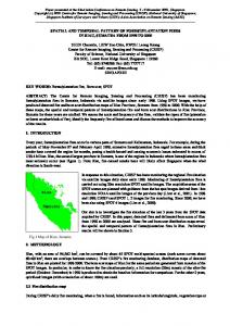
where V, is volume (thousands of board-feet, mbf) per acre on stand s for trees of age t,Y, and K,v is the carrying capacity of land on stand s. Table I lists’base-level parameter values. The timber function is depicted in figure la for alternative values of 8,$. The nontimber benefit function has two parts. First the forage production function is

s=l.Z

where g, estimates forage production from stand s in animal-unit-months (aum) per year. The forage production function (8) is depicted in figure lb for alternative values of pas. Second, the value of the forage is an inverse function of the quantity of the forage, as given by ( 9 ) f(t,,, t2n) =

fO~~Y[R,(‘,.)+~z(‘2”)1

where f0 represents the upper bound on the value of the forage and defines an adjustment rate for the availability of forage in the forest. Table 1 lists the values forfo and y that yield marginal forage values ranging from $8.00 to $29.00 per aum. The marginal valuation function, f(t,,,. t2,J reflects demand for hunting sites and the response of wildlife to forage and cover supplies. For example, if the ecosystem has enough cover for wildlife but not enough food, then the marginal value of increasing forage is high. Both stands produce nontimber benefits, since wildlife migrate across the stands, so the nontimber benefit function is simply the product of forage production (8) and its marginal valuation (9): (10) a(t,,, t2J = ]R,(fIJ + g*(L)1 .f(fI,. f2n). Figure lc illustrates the nontimber benefits obtained from the whole forest ecosystem. For example, when at least one stand, here stand 2, is held, hypothetically, in a constant condition that is intermediate between both cover production and high forage production (e.g., with a constant tzn = 25), the nontimber benefits ob-

316

A m e r . J. Agr. Econ.

May 1997

1

16

31

46

61

76

91

106

121

136 151 166 181 196

Age of the Stand

1

5

9

13 17 21 25 29 33 37 41 45 49 53 57 61 65 69 73 77

Age of the Stand

5.6

0 1

5

9 13 17 2 1 25 29 33 37 41 45 49 53 57 6 1 65 69 73 77

Age of Stand 1, tl, Figure 1. Timber (a) and forage (b) production and nontimber benefit (c) functions for a twostand ecosystem

Swallow, Talukdar, and Wear

tained from the forest ecosystem are quite high because the other stand may add a substantial quantity of forage when the forage value is relatively low; but, as that stand ages, it provides cover while stand 2 still provides sufficient forage (figure lc). With table 1, the timber model described in equation (7) has its maximum growth rate at age 60 and the harvest age that maximizes timber benefits alone (the Faustmann age) is 76 years. The base-case simulation assumes that ages after 80 on either of the two stands are not relevant to the optimization. This boundary assumption reduces the computing burden and is not a binding constraint since the timber-only optimum occurs before age 80 and nontimber benefits encourage younger harvest ages. The simulations using the base timber model (7) (with table 1) consider stand ages in one-year increments ranging between 0 and 80. The state variable, t, in equation (6), represents the initial ages of the forest stands at the beginning of the year n. Then t, is an element of a vector cp of possible vectors for the initial ages of the two stands; the dimension of cp is 8 l2 x 1 as we include age 0 as a possibility. We also report sensitivity analyses where the timber model (7) involves slower growth [figure 1, 8 = 0.06408 for equation (7)], and in these cases we assumed growth on the stands could be relevant to age 90 since in these cases the timber-only optimum would have been 88. In these cases of slower timber growth, we set the boundary constraint to 90, so that $I had dimension 912 x 1. Again, this boundary assumption reduces the computing burden but does not constrain the optimization; sensitivity analyses with boundary assumptions up to 100 had no impact on the solutions.

Forest Ecosystem Management

317

sensitivity analyses reveals that managers may be unable to use rules of thumb to address real ecosystem management issues, but the model provides a framework that may aid in many situations. In the sensitivity analyses, the key parameters of the timber (E),) and nontimber (&,,) functions are lowered by 20%, in various combinations across the two stands, to produce scenarios for comparison with the base case. We identify each scenario by an expression of the form Tim,Ntim, - Tim,Ntim,, where Tim, indicates whether the timber productivity on stand i is at the base-case level (Tim, = B) or at the lower level (Tim, = L), and Ntim, indicates whether nontimber productivity on stand i is at the base-case level (Ntim, = B) or at the lowered level (Ntim, = L). For example, BB-BB identifies the base case itself, but BL-LB identifies that stand 1 has base-case timber but lower forage and stand 2 has lower timber growth but base-case forage production. Accordingly, table 2 outlines ten scenarios for the present discussion, including a base case and nine sensitivity analyses. In every case, the optimal management regime is defined by a transition sequence of harvests followed by an infinitely repeating steady-state harvest sequence. The steady-state sequence incorporates a finite number of harvests over a finite period q such that the stand ages immediately after the steady-state sequence are the same as existed when the steady-state sequence began. For example, if calendar time c is the period at which the ecosystem first begins a cycle through the steady-state sequence, then the vector of stand ages, t,, satisfies the condition

(11) t, = tc+q+l Simulation Results In this section we provide an empirical illustration using the timber and nontimber functions (7)-( 10) and a 4% discount rate. First, the basecase simulation involves two stands that are identical in both timber and nontimber production, using equations (7)-(10) and parameters in table 1 for both stands, setting the initial ages of the two stands to zero (initially, bare soil). Then, to assess the implications of the model, we report several sensitivity analyses using different scenarios. These analyses revealed that the optimal harvest patterns in the ecosystem are sensitive to the key parameters that represent timber and nontimber productivity levels on each stand. Comparison across

and the set of optimal decisions implemented during the sequence is repeated over the period of the steady state, so

(12)

ix:, x,‘+,, . . . , x:+,1 = K+q+,’Xfcq+2 ... 9 xi+21j+,).

The transition sequence consists of all harvests prior to calendar time c. Note that, while our simulations involve two stands, the steady-state conditions (ll)-(12) apply in the general case (S > 2). For the ten scenarios, the results are elaborated below and summarized in table 3 and figures 2-4. They show that shifting the timber and nontimber productivity levels generally

318

A m e r . J. Agr. Econ.

May 1997

Table 2. Definition of Simulation Scenarios Stand 2 Production Functions Stand 1 Production Functions Timber B B L L

Nontimber B L B L

B B

B L

L B

L L

BB-BB

BB-BL BL-BL

BB-LB BL-LB LB-LB

BB-LL BL-LL LB-LL LL-LL

Timber: NonTimber:

Note: Production functions are defined for a base case (“B”) and a low case (“L”) for each stand. For timber production, the L-function sets 8, to (0.80)(0.0801) (see figure la; table I). For nontimber production, the L-function sets PO\ to (0.80)(0.0770) (see figure lb; table 1).

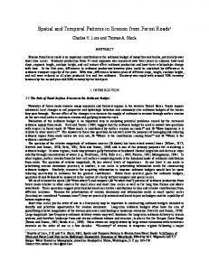
leads to qualitatively different management regimes on the two stands. The figures appear complex, but these graphs illuminate the relationship of timber growth to the concurrent flow of nontimber benefits. Each graph contains two components. The first component consists of nonlinear curves which constitute iso-value contours for nontimber benefits; i.e., the iso-value contours define level planes of a(t,,, t2J. The second component consists of straight lines that track the ages of each stand as timber grows and is harvested. For example, figure 2a shows a timber growth pattern beginning with both stands at age zero; both grow to age 38 when stand 1 is harvested, and the horizontal dashed line shows that timber growth continues from where stand 1 is age zero and stand 2 is age 38; both now grow until stand 1 reaches age 35 and stand 2 is age 13; then stand 2 is harvested and growth continues from where stand 1 is age 35 and stand 2 is age 0. In this way, diagonal lines pertain to periods of growth and horizontal or vertical lines pertain to harvest on one stand. For each scenario discussed below, diagonal dotted lines represent timber growth in the transition sequence and diagonal solid lines represent timber growth during steady state.

Scenarios Parameterized with Identical Stands

To begin, we first consider how management changes in the four scenarios on the diagonal of table 2, which vary productivity but focus on identical stands. Results for these scenarios are graphed in figure 2. First, we consider the base case. With the base case applied to both timber and nontimber productivity, scenario BB-BB, the transition phase is defined by a single harvest after 38 years (table 3). The steady state then involves alternate harvests at age 73 on both

stands. Inclusion of nontimber benefits leads quickly to a Hartman-style rotation; that is, the early nontimber benefits give rise to a rotation that is shorter than the Faustmann age of 76.4 In this model, however, such a harvest age is established after a transition staggers the harvests on the two stands, optimizing the combination of timber and nontimber. From figure 2a we see that, in the steady state, timber harvests are staggered so that the stands grow through the range of higher iso-value contours for nontimber, growing no lower than the iso-value line “3.” Clearly, both timber and nontimber values are compromised in this case, since timber values are compromised by a transitional harvest at about half the Faustmann age, as well as by a Hartman-style rotation in steady state, while the growth phases do not maintain nontimber values within the highest one or two isovalue contours. However, as we follow the scenarios along the diagonal in table 2, a more complex complement of harvest sequences arises. In scenario LB-LB (table 3, figure 2c), the ratio of timber to nontimber benefits is lower and stands alternate, temporally, between short (twenty-fiveyear) rotations specializing in forage and long (eighty-one-year) rotations specializing in timber production. With a lower opportunity cost of foregoing timber harvest benefits, this steady state staggers the harvests more carefully so the stand ages more closely follow the ridge of high nontimber values. Even though the stands remain identical, and the lower productivity for timber (relative to BB-BB) means ecosystem links cause management to shift toward nontimber benefits, results show some steady-state rota-

4 In this case, nontimber production peaks at a young age (figure lb), so Hartman’s model anticipates a rotation shorter than that of Faustmann.

Forest Ecosystem Management

Swallow, Talukdar, and Wear

319

Table 3. Harvest Sequences for a Simulated Two-Stand Forest Ecosystem with Alternative Scenarios for Timber and Nontimber Production, Assuming the Two Stands Begin with Bare Soil Scenario Name” (figure) Stand BB-BB Ga, 3a)

2

BB-BL (3b)

1 2

BL-BL (2b)

1 2

I

BB-LB (3c)

1 2

BB-LL (3d, 4a)

1 2

BL-LB (-)

1 2 1 2

BL-LL (4b)

Age of Stands for Each Successive Harvest on the Ecosystem 38 13 (0.38) 36 nh (0,35) 12

67

(38.0) ah (0,37)

76 22

13

25

53

73 (0.35) 13 (3690) 75

24

74 w (0325)

24 (25,O)

48

Bh (2430)

74 22

53

24

24

(49,O) 74 (48,O)

74 24

1 2

26

LB-LL (4c)

1 2

22

LL-LL (2d. 4d)

1 2

22

45

25

24

LB-LB (2c)

40

25

26b cW0)

48 (0,28) 75

(3YO) ah

(59.0)

22b (15,O) 82

26

(468)

25 23

36

(0,28) 23b

81 (0,53) 24

85 (0,18)

-

73 (0.37)

(41,O)

26 (20,O) 31 (0,16) 25 (2830) 85 (0965)

22 (15.0) 81

25

(53,O) 38

(0.28)

(20,O)

(0.18)

2

3

26 35

-

-

26 (0,13)

(13,O)

I followed by stand 2. “B” represents base-case productlvlty, while “L” represents a case of lower productivity. ’ Underline indlcatrs start of the steady-state cycle. Numbers in parentheses mdicate the values of stand ages f,, and f,, where n is the period immediately following the preceding harvest. For example, in scenario BB-BB, after the first harvest on stand I at age 38, the state of the ecosystem is (0, 38) since stand 1 returns to bare soil while stand 2 remains unharvested; this state leads to the first harvest in the steady-state cycle at age 73 on stand 2; this state is repeated after the last harvest in the steady-state cycle. ’ Defined by table 2. Pairs of letters represent timber and nontimber production functions, respectively, on stand

tions that specialize stands in a varying pattern over both space and time. In scenario BL-BL, timber productivity is held at the base level but forage productivity is reduced on the two stands (figure 2b). The eventual steady state is nearly identical to the base case, but the transition sequence is very different, requiring a total of 169 years (BL-BL) rather than only 38 years (BB-BB) (table 3, figures 2a-b). In scenario BL-BL, relatively higher timber opportunity costs increase the time in transition to a steady state. Of course, this steady state still staggers harvests to enhance nontimber benefits, but it does so after balancing the delay in reaching the steady state with the greater timber benefits obtained during the transition. In scenario LB-LB, the nontimber values are actually helped by an apparent “timber-

emphasis” harvest. However, a timber emphasis is not really justified with the lower timber growth function since the timber-emphasis harvest disappears when the relative nontimber benefits are lower (compare LBLB and LL-LL, figures 2c-d). That is, the harvest of mature timber in scenario LB-LB appears optimal due to nontimber considerations rather than the profitability of timber per se. This result confirms the informal intuition that ecosystem management for nontimber goods may still involve timber harvests in some cases. Such timber harvests may even appear to be “below cost” if their nontimber benefits are ignored; harvests of mature timber are no longer part of optimal management in scenario LL-LL despite the same timber productivity as in scenario LB-LB (fig-

320

May 1997

A m e r . J. Agr. Econ

a. Scenario BB-BB.

- 0

15 30 45 60 75 A g e o f S t a n d 1 (tI,)

90

Scenario LB-LB

0

15

30

Age of

b. Scenario BL-BL.

15 30 45 60 75 A g e o f S t a n d 1 (t,,)

C.

45 60 75 S t a n d 1 (tl,)

90

d. Scenario LL-LL.

90

15

30

Age of

45 60 75 S t a n d 1 (tl,)

90

Note: Straight diagonal lmes show the age of stand 1 relative to the age of stand 2 during a steady-state cycle (sohd lines) and a transition sequence (dotted lines). The straight vertical and horiamtal dashed linea indicate an mstantaneous fall in one stand’s age due to a harvest of that stand.

Figure 2. Overlay of timber growth and harvest patterns on iso-value contours of the nontimber benefit function a(t,,, f2,J for scenarios with identical stands me 2, table 3).5 Conversely, since scenario LLLL includes no harvests of mature timber, the results illustrate that nontimber ecosystem benefits may justify foregoing commercially viable timber rotations, which, in this case, would occur with the Faustmann age of 88. The relative value of timber production in this case is not high enough to offset forgone nontimber production. 5 With low (L) timber productlwty, the Faustmann age is still nonzero and finite, so the point, concerning “below cost” sales, is offered generically, rather than specifically.

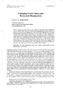
Scenarios Parameterized with Base-Level Productivity on Stand I We next consider the set of four scenarios defined by the first row in table 2 (figure 3). For these scenarios, stand 1 is held at the base case while the relative productivities on stand 2 are varied, simulating nonidentical stands. When timber productivity alone is lowered on stand 2 (BB-LB, figure 3c), the optimal steady-state harvest sequence for stand 1 is essentially identical (73 or 74 years). That is, the

Swallow, Talukdur, and Wear

a. Scenario BB-BB.

Forest Ecosystem Management

321

L.

Scenario BB-LB.

A g e o f S t a n d 1 (tl,)

A g e o f S t a n d 1 (tI,)

b. Scenario BB-BL.

d. Scenario BB-LL.

A g e o f S t a n d 1 (tl,)

A g e o f S t a n d 1 (t,,)

N o t e : S t r a i g h t dmgonal lines show the age of stand I relative to the age of stand 2 durmg a steady-state cycle (solid lines) and a transition sequence (dotted lines). The straight vertical and horizontal dashed hnes indicate an instantaneous fall in one stand’s age due to a harvest of that stand. Panel (a) reproduces figure 2a.

Figure 3. Overlay of timber growth and harvest patterns on iso-value contours of the nontimber benefit function a(t ,“, t2,,) for scenarios holding stand 1 at base-case productivity level difference in the productivity of one stand (stand 2) does not change management on the other (stand 1) when the other is defined by relatively high base levels of productivity. In contrast, management on stand 2 is affected. For example, lowering the relative productivity of timber on stand 2 leads to a qualitative shift in management on stand 2 (i.e., when moving from BB-BB to BB-LB and from BB-BL to’ BB-LL; figure 3); however, shifting relative forage productivity on stand 2 leads to only subtle changes in har-

vest patterns on stand 2 (i.e., patterns when moving from BB-BB to BB-BL and from BBLB to BB-LL remain qualitatively unchanged; figure 3). In this example (figure 3, table 3), management adapts to differing relative productivity levels across stands by altering the harvest schedule on the stand with lower productivity for one of the two output types. The altered schedule may even involve consecutive harvests on one stand without an intervening harvest on the other.

322

A m e r . J. Agr.

May 1997

Scenarios Parameterized with Low-Level Productivity on Stand 2 However, when the simulations hold one stand (stand 2) constant at lower productivities for both forage and timber (last column in table 2, figure 4), the results are much different. With low productivity for both output types on both stands (scenario LL-LL), the steady state focuses on nontimber production. However, when the timber productivity on stand 1 is raised to the base level (BL-LL), then an almost “pure” specialization results (figure 4b): stand 1 specializes in the production of saw timber (harvest age of 75), while stand 2 specializes in the production of forage and pole timber (harvest ages of 30, 22, and 22) (table 3). A more substantial shift in harvest patterns results when only the forage production function is raised to the base level on stand 1 (LBLL). When this occurs, the steady-state harvest sequence on stand 2 shifts from a very short rotation (26 years in figure 4d) to a very long rotation (85 years in figure 4c) which approaches the Faustmann age of 88. When one stand is held at the lower productivity levels, differences in the productivity of the other stand can have a substantial influence on its management, a result that counters intuition from existing models and may help to develop rules for defining adjacency constraints as proposed by Roise. In addition, this case illustrates that increased productivity of nontimber on one stand may lower the relative value of nontimber production on another stand, via substitution effects (Swallow and Wear), leading management to emphasize timber production on a stand where managers would have emphasized nontimber if the ecological context had differed (compare figures 4d and 4~). Nonoptimality of constant rotations. It bears emphasizing that management plans do not necessarily reduce to a constant rotation age over time, nor do they reduce to some other simple rule of thumb based on site productivity. Rather, management of a stand depends significantly on its context in the forest, including how its ecological role is influenced by its location relative to other stands. While a multiplestand model with nontimber benefits (e.g., Bowes and Krutilla 1989, pp. 128-29) may eventually settle into a steady state that approaches a Faustmann-Hartman type of decision rule, such a rule generally will not hold when location explicitly affects ecosystem benefits (see appendix). Scenario LB-LB provides an example: the steady-state cycle satisfies the

Econ.

general optimality condition from the entire forest by balancing the marginal benefits and marginal opportunity costs of delaying each harvest (see appendix). Individual harvest ages are not constant for each stand, even in the steady state, although a collection of rotations will repeat in the steady-state cycle (table 3). In general, sequential harvests occur at different ages because a harvest on any stand s changes the condition of the forest surrounding every other stand and the optimality condition includes terms for a feedback from each harvest age onto present and future harvest ages for the other stands. The model thus provides an approach which tracks the changes in the forest condition once a harvest decision is implemented in one part of the ecosystem and then optimizes the harvest schedules in other parts of the ecosystem by adjusting for these changes in forest condition. Sensitivity to initial conditions. Results presented here all assumed the two-stand ecosystem began as bare soil, represented as an initial condition with t,, = 0 for s = 1, 2. Sensitivity to this assumption was assessed through selected scenarios where initial conditions on stand 2 remained with bare soil, but the initial age of stand 1 varied, Results showed that initial conditions may dramatically alter the optimal transition sequence and may also alter the optimal steady-state cycle, although the latter effect was less dramatic. For example, in the base case (BB-BB), if stand 1 begins initially at age 12, the transition sequence involves not one harvest, as in table 3, but rather it involves fourteen harvests. In this example, the age of harvest during the transition begins at age 67 on stand 1, rather than 38 as in table 3, and it rises steadily to the familiar steady-state harvest age of 73; meanwhile, the age of harvest on stand 2 begins at age 76 and declines to the familiar steady-state harvest age of 73. In contrast, if the initial condition of stand 1 is reduced only two years, to age 10, then the transition still involves only one harvest as in table 3, although now that harvest is at age 27 on stand 2. The ecosystem achieves a steady state with harvests of age 73 on both stands, but the harvests are now staggered on a slightly different schedule ([t,,, tzn] begin the steady-state cycle at ages [37, 01, followed by ages [O, 361, followed by the next cycle through the steady state). Conclusions In this paper we develop a model for the standlevel forest management problem in which geo-

Foresi Ecosystem Management

Swallow, Talukdar, and Wear

a. Scenario BB-LL.

- 0

15 Age

30

45

60

75

90

C.

Scenario LB-LL.

0

of Stand 1 t(l,)

15 Age

30

45

60

75

15

30

45

60

75

90

Age of Stand 1 t(l,)

b. Scenario BL-LL.

- 0

323

90

of Stand 1 t(i,)

d. Scenario LL-LL.

0

15

30

45

60

75

90

Age of Stand 1 t(i,)

Note: Straight diagonal lines show the age of stand 1 relative to the age of stand 2 during a steady-state cycle (solid lines) and a transition sequence (dotted lines). The straight vertical and horizontal dashed lines indicate an instantaneous fall m one stand’s age due to a harvest of that stand. Panel (d) reproduces figure 2d.

Figure 4. Overlay of timber growth and harvest patterns on iso-value contours of the nontimber benefit function a@,,, t2J for scenarios holding stand 2 at lower productivity level graphically distinct stands may be ecologically interdependent and managed by a single decision maker. This model is developed conceptually for a general case with any number of stands and it maintains the potential for ecological production to depend on the geographic location of different stands. The model is assessed using simulations for the simplest case of a two-stand forest ecosystem. Importantly, the simulation results show a number of departures from the “rules of thumb” based on models with independent stands. First,

even with identical ecological production of both timber and nontimber on both stands, the harvest rotations in the transition sequence (prior to the steady state) may be quite different on the two stands. A longer rotation age in one stand may occur to compensate for the lack of concealing cover for wildlife when the other stand is younger. This result may be the first numerical illustration of potential gain from specialization; these gains may arise because timber and nontimber goods may respond differently to management actions (Vincent and

324

A m e r . J . Agr. Econ.

May 1997

Binkley).6 Second, the results show that it is possible to have one stand harvested consecutively while the other is left to provide cover for wildlife (table 3) and then harvested for saw-timber quality logs. In fact, in some cases it may be that nontimber benefits justify occasional saw-timber quality harvests. Thirdly, the optimal harvest schedule in the multiple-stand ecosystem management problem does not necessarily converge to the single-stand solution of the traditional Hartman-type forest management models. Within the steady state, specialization across stands may significantly lower the harvest age for one stand while the other stand is allocated for longer rotations that capture the benefit of timber sales. Although each harvest age balances the marginal benefit of delaying a harvest against the marginal opportunity cost of delay, the ecosystem interdependencies generally imply that the “rotation” of harvests on the single stand may not occur according to a constant interval or period in time. Depending on the surrounding forest conditions, then, the optimum harvest schedule for one stand may differ significantly, so locational identity of a stand plays a role that cannot be captured in a model that simply tracks multiple independent stands. Previously, the gains from staggered harvests have been approached by using models with multiple, independent stands in combination with a collection of ad hoc constraints on the timing of adjacent harvests (e.g., Roise). In the long run, our model may aid in development of a more complete ecosystem management planning tool; in the short run, the present simulation approach may provide insights into identifying ecosystem factors for which different adjacency constraints are appropriate. Our simulation results indicate that the nature of the stand interactions, including the resource managers’ objectives, may alter the optimal management plan substantially. By extending traditional forest management models to account for system-level effects, the present model assesses the returns to specializing over time as well as over space and shows how those returns affect the pattern of an optimal harvest plan. Resulting management plans may allocate a particular forest area to different roles over time, rotating a stand’s productive emphasis across different resource uses, rather than es-

’ “Specialized” stands may still contribute to both timber and nontimber values, but their relative contributions to these values determine a degree of specialization.

tablishing specialized land-areas with time-invariant timber or nontimber emphases. With respect to the timing of harvests across an ecosystem, our results suggest the following observations: when the stands are of similar (or identical) productivity and (i) when the productive value of timber is low relative to that of nontimber values, optimal plans tend to stagger harvests more carefully to enhance nontimber values, but (ii) when nontimber values are low relative to timber, the transition time may increase prior to achieving staggered harvests to enhance nontimber values; when one stand is relatively more productive in timber or nontimber, (iii) management of that stand accounts for ecological linkages, but may not be sensitive to shifts in productivity of a less productive stand, while, conversely, (iv) management on the less productive stand may be sensitive to shifts in productivity of the more productive stand. However, because management of each stand depends upon the qualities of its ecological neighbors, because endogenous management choices change these qualities over time, and because optimal harvest patterns on each stand may differ markedly, even for identical stands, the optimal management pattern on any individual stand or on any set of stands appears to require specific analysis rather than dependence upon simple rules of thumb. A natural extension of this work is to develop more comprehensive forest-level models, to support actual planning analysis, through such methods as decomposition algorithms (Berck and Bible). Our model may also provide a benchmark for game-theoretic analysis applied to forests under independent managers (compare Munro 1979, 1990) where the objectives of land owners may differ or conflict. Since real ecosystems may involve multiple landowners controlling one or more “management units,” such future applications address a core challenge of ecosystem management. [Received February 199.5; final revision received January 1997. ]

References Behan, R.W. “Multiresource Forest Management: A Paradigmatic Challenge to Professional Forestry.” J. Forestry 8(April 1990): 12-18. Berck, P., and T. Bible. “Solving and Interpreting Large-Scale Harvest Scheduling Problems by Duality and Decomposition.” Forest Sci. 30(March 1984): 173-82.

Foresi Ecosystem Management

Swallow. Talukdar. and Wear

Bowes, M.D., and J.V. Krutilla. “Multiple Use Management of Public Forest Lands.” Handbook of Nutural Resource and Energy Economics, vol. II. A.V. Kneese and J.L. Sweeney, eds. Amsterdam: North Holland, 1985. Bowes, M.D., and J.V. Krutilla. Multiple Use Management: The Economics of Public Forest Lunds. Resources for the Future. Washington DC: Resources for the Future, 1989. Calish, S., R.D. Fight, and D.E. Teeguarden. “How Do Nontimber Values Affect Douglas-Fir Rotations?” J. ForestT 76(April 1978):217-21. Faustmann, M. “On the Determination of the Value which Forest Land and Immature Stands Pose for Forestry.” Martin Fuustmunn and the Evolution of Discounted Cash Flow. M. Cane, ed. Oxford: Oxford Institute, 1968. Franklin, J.F., and R.T.T. Forman. “Creating Landscape Patterns by Forest Cutting: Ecological Consequences and Principles.” Lundscupe Ecology 1(1987):5-18. Giles, R.H. Wildlife Management. San Francisco CA: Freeman, 1978. Hartman, R. “The Harvesting Decision When a Standing Forest Has Value.” Econ. Inquiry 14(March 1976):52-58. Hof, J.G., and L.A. Joyce. “Spatial Optimization for Wildlife and Timber in Managed Forest Ecosystems.” Forest Sci. 38(August 1992):489-508. Johansson, P., K. Lofgren, and K.G. Maler. “Externalities in Consumption, Pareto Optimality and Timber Supply.” Unpublished manuscript, The Swedish University of Agricultural Sciences, Department of Forest Economics, Umea, Sweden, 1988. Kennedy, J.O.S. Dynamic Programming: Applicutions to Agriculture und Nutural Resources. New York: Elsevier Applied Science Publishers, 1986. Munro, G.R. “The Optimal Management of Transboundary Fisheries: Game Theoretic Consideration.” Nut. Resour. Modeling 4(Fall 1990):403-26. _’ “The Optimal Management of Transboundary Renewable Resources.” Can. J. Econ. 12(August 1979):355-76. Newman, D.H. The Optimal Forest Rotation: A Discussion und Annotuted Bibliography. U.S. Department of Agriculture, Forest Service General Tech. Rep. SE-48, Southeastern Experiment Station, 1988. Parades, G.L., and J.D. Brodie. “Land Value and the Linkage Between Stand and Forest Level Analyses.” Land Econ. 65(May 1989): 158-66. Roise, J.P. “Multicriteria Nonlinear Programming for Optimal Spatial Allocation of Stands.” Forest Sci. 36(September 1990):487-501.

325

Swallow, S.K. “Economic Issues in Ecosystem Management: An Introduction and Overview.” Agr. und Resour Econ. Rev. 25(0ctober 1996):83-100. Swallow, S.K., P.J. Parks, and D.N. Wear. “PolicyRelevant Non-Convexities in the Production of Multiple Forest Benefits.” J. Environ. Econ. and Manage. 19(November 1990):264-80. Swallow, S.K., and D.N. Wear. “Spatial Interactions in Multiple Use Forestry and Substitution and Wealth Effects for the Single Stand.” J. E n v i r o n . Econ. and Manuge. 25(September 1993):103-20. Vincent, J.R., and C.S. Binkley. “Efficient MultipleUse Forestry May Require Land-Use Specification.” Lund Econ. 69(November 1993):370-76. Wear, D.N., and S.K. Swallow. “The Economics of Location and Forest Management for Multiple Benefits: A Review, Discussion, and Speculation.” Modeling Sustainable Forest Ecosystems: Proceedings of a Conference in Wushington DC, November 18-20, 1992. D.C. LeMaster and R.A. Sedjo, eds. American Forests, Washington DC, 1993.

Appendix Marginal Conditions for Harvests This appendix shows that, at the time of each harvest on each stand, the optimality conditions balance the marginal benefits of a small delay (MBD) of the harvest against the marginal opportunity costs of that delay (MCD). In the multiple-use context, this balancing was first suggested by Hartman; this appendix shows how other aspects of the Hartman-type rotation arise in the present model. First, we note that objective (3) replicates the objective studied by Swallow and Wear (see also Wear and Swallow), for a single stand, by summing over multiple stands; we rewrite equation (3) as

(A.])

where

R(T,,) = pV,r(T,,)exp(-rT,,) 1 al (t,,Tt, ) exp(-rt,)dt,

and ax,yz = exp(-rCT,), 0 < y - 1 < Z, with CI,,,,_, = 1 and %,y+m %+m+l,r = a,,z for any nonnegative integer m. Using (A. l), the first-order condition for the rotation age for some rotation k on some stand s’ is

326

(A.21

May I997

A m e r . /. Agr. Econ.

6@/6T,,, = (pi5V,J6Ts,, + a,JTs8,, T,) - vV,~(T,~,)l%,,., + 6Y.~,.k+,.J6T,,,

+

1)

6Y’,,,,,16T,~,= 0

where Y’,.,,,n is the summation over i in (A.1) (inside the braces), where i runs from m to n (and IZ may be -) and where 6Y’,,,,n/6T,,, = 0 if harvest n on stand s (S # s’) occurs earlier in calendar time than harvest k on stand s’. This first-order condition (A.2) requires a balance between MBD and MCD but it includes not only the terms in Swallow and Wear but also an adjustment that recognizes how a marginal delay in harvest i on stand s affects nontimber benefits received from all other stands over the future after harvest i on stand s. Condition (A.2) may be rewritten as

(A.3)

MBD,, = MCD,,, -

c 6Y,,,,J6Ts,k = 0 S=I,S#S’

where MBD,,, and MCD,?,, capture the terms considered by Swallow and Wear while the remaining term accounts for additional wealth effects of the impact of a marginal increase in T,, on future nontimber benefits from other stands; these remaining terms become part of MCD in the present model.7 Thus, the optimal harvest age on each stand for each harvest balances MBD and MCD, so that the age is a Hartman-like optimal age. However, since T,, # T,

’MCD,., equals rpV,,(T,&x,~ , k and MBD,., captures the remaining terms from equation (A.2) that are no longer explicit in equation (A.3).

for i # j, in the general case, one cannot conclude that the Hartman model has additional generality; this conclusion contrasts with Bowes and Krutilla (1989, pp. 128-29) who omit locational identity. Moreover, each steady-state cycle covers a finite period. We defined (above) q as the calendar-time period of a steady-state cycle and c as the calendar time at which one of these cycles begins. Recall that the steady-state cycle consists of a sequence of harvests such that the state of the ecosystem at the start of that sequence (one instant after the last harvest preceding that sequence) is reestablished immediately after the last harvest in that sequence: (A.4)

1, = G+ll fE

where E represents one marginal increment (one moment) in time, so that equation (A.4) establishes a continuous-time version of the analogous condition in the discrete time dynamic program [equations (1 I)-( 12) above].* Therefore, the end of the period n coincides with an optimal harvest age, so that the optimal length of q also balances the MBD against the MCD associated with a marginal increase in the length of the steady state. In the ecosystem management model here, it is n that matches most closely with the repeated period of a harvest obtained in the Hartman m o d e l ; Hartman’s “rotation age” T coincided with both the harvest age on the individual stand and the period of the steady state, but, in general, this coincidence no longer holds in an ecosystem management context.

’ We still assume that the steady-state cycle consists of a finite number of harvests from the ecosystem, despite the focus here on continuous time. This assumption is valid for the discrete time dynamic program in the text, but it may not hold in continuous time. However, the point of the appendix does not require further analytical precision.