Spatial and temporal patterns of forest disturbance and regrowth ...

Remote Sensing of Environment 122 (2012) 117–133

Contents lists available at SciVerse ScienceDirect

Remote Sensing of Environment journal homepage: www.elsevier.com/locate/rse

Spatial and temporal patterns of forest disturbance and regrowth within the area of the Northwest Forest Plan Robert E. Kennedy a,⁎, Zhiqiang Yang a, Warren B. Cohen b, Eric Pfaff a, Justin Braaten a, Peder Nelson a a b

Department of Forest Ecosystems and Society, Oregon State University, United States USDA Forest Service, PNW Research Station, United States

a r t i c l e

i n f o

Article history: Received 2 March 2011 Received in revised form 19 September 2011 Accepted 20 September 2011 Available online 13 February 2012 Keywords: Change detection Landsat Forest Northwest forest plan Disturbance Growth

a b s t r a c t Understanding fine-grain patterns of forest disturbance and regrowth at the landscape scale is critical for effective management, particularly in forests in western Washington, Oregon, and California, U.S., where the policy known as the Northwest Forest Plan (NWFP) was imposed in 1994 over > 8 million ha of forest in an effort to balance environmental and economic tensions. We developed approaches to create disturbance and regrowth maps for forests within the area of the NWFP from the results of LandTrendr, a temporal segmentation algorithm described previously only at the pixel scale. Maps were developed from 674 Landsat Thematic Mapper and Enhanced Thematic Mapper + images distributed across 22 separate scene areas, and were assessed for validity at 2360 points using TimeSync, a time-series validation and interpretation tool. Unlike maps derived using other techniques, maps derived from the segmentation approach were unique in providing simultaneous detection of abrupt disturbance, chronic disturbance, and ongoing vegetative growth with consistency across large areas and across time. Maps were then used to address six core monitoring questions focusing on the distribution of disturbance across time, ownership categories, and ecoregions. Forest was disturbed at rates that varied by ownership category and state, ranging from 9% to >39% of forest area over the period 1985 to 2008, with highest cumulative disturbed area on private and native lands in Washington and Oregon and lowest disturbed area on federal protected lands in Washington. Effects of court injunctions and subsequent implementation of the NWFP lowered forest disturbance rates, particularly in Oregon, and also caused decreases in the relative magnitude of disturbance on those lands relative to private lands. Statemanaged forests showed forest disturbance rates that varied considerably among the three states, with the highest rates in Washington state and lowest in California. Affected by large, stochastic fire events, protected lands in both Oregon and California showed disturbance rates similar to those found on actively managed federal lands. Protected lands also experienced high rates of chronic disturbance, often associated with insect-related mortality. As expected, moisture-limited ecoregions recovered vegetation more slowly than those where moisture was not limiting. Vegetative regrowth rates showed substantial variation among ownership categories, suggesting that differential forest policies may affect vegetative recovery rate. Taken together, these results emphasize that forest management policies do have manifestations at the landscape scale, but that detection of these manifestations is best achieved with mapping approaches that can detect both abrupt and longer-duration processes within the Landsat archive. © 2012 Elsevier Inc. All rights reserved.

1. Introduction As humans grapple with increasing domination of Earth's processes (IPCC, 2007; Vitousek et al., 1997), a central challenge lies in understanding how human decisions made at relatively local scales manifest themselves as changes at broader scales. While common pressures of economics, policy, and geography may elicit similar responses from individual actors (Lambin et al., 2001, 2006), landscapes are composed of a mix of individuals and institutions with different pressures, leading

⁎ Corresponding author. Tel.: + 1 541 7507498. E-mail address: [email protected] (R.E. Kennedy). 0034-4257/$ – see front matter © 2012 Elsevier Inc. All rights reserved. doi:10.1016/j.rse.2011.09.024

to a geographic mosaic of change (Ramankutty et al., 2006; Turner et al., 2007). The pressures acting on those individuals and institutions are themselves in flux, as economic, social, political, and natural processes change over time. This spatial and temporal mosaic of change processes affects any ecosystem service that integrates across a landscape, including delivery of water, maintenance of biodiversity, support of local economic systems, provision of recreational opportunities, etc. (DeFries et al., 2004; Lambin & Geist, 2006). Wise decision-making ultimately rests on understanding the linkages between constraints, changes, and resultant impacts (Reid et al., 2006; Verburg et al., 2006). Developing that understanding, in turn, requires that landscape changes be characterized at spatial and temporal scales commensurate with the actors and the pressures on those actors (Turner et al., 2007).

118

R.E. Kennedy et al. / Remote Sensing of Environment 122 (2012) 117–133

With their synoptic view of the Earth's surface, satellite-based sensors often play a role in characterizing landscape change (Coppin et al., 2004; Frolking et al., 2009), but the Landsat family of sensors are particularly well-suited for this effort (Goetz, 2007; Ramankutty et al., 2006). Landsat Thematic Mapper (TM) data (including, for ease of reference, data from the Enhanced Thematic Mapper Plus, or ETM+, sensor) have a spatial grain small enough to resolve many human-scale patches (fields, roads, etc.) and a spatial extent large enough to map landscapes (Cohen & Goward, 2004). Thus, they not only have the potential to detect the manifestation of individual land management decisions, such as urban development or forest harvest, but also the capacity to do this over areas large enough that many such events can be detected and that possible patterns can be revealed (Ramankutty et al., 2006). More importantly, however, these changes can be tracked over many economic, political, and climatic cycles because the Landsat Thematic Mapper (TM) image archive stretches back to 1984 (Wulder et al., 2008). Extracting information from this archive became significantly easier when the Geological Survey (USGS) began providing all Landsat data freely, with a consistent and robust radiometric and geometric recipe (Woodcock et al., 2008). With this significant barrier to processing removed, analyses based on multiple Landsat images, long a staple in the literature (Garcia-Haro et al., 2001; Guild et al., 2004; Hayes & Sader, 2001; Healey et al., 2008; Hostert et al., 2003a, 2003b; Lawrence & Ripple, 1999; Sader et al., 2003; Viedma et al., 1997), are likely to increase in number and efficacy, as the recent proliferation of such studies would suggest (Goodwin et al., 2010; Hais et al., 2009; Huang et al., 2010; Powell et al., 2008; Powell et al., 2010; Roy et al., 2010; Schroeder et al., 2011; Sonnenschein et al., 2011; van Lier et al., 2011; Vogelmann et al., 2009). While the Landsat archive may contain rich information on land change at appropriate spatial and temporal scales, the challenge is distilling from the long archive only the important features of change. With a deep historical reach, Landsat data have the potential observe a wide range of processes, ranging from events that are abrupt and unambiguous, such as those caused by land clearing for development (Helmer et al., 2010; Powell et al., 2008), resource extraction (Almeida & Shimabukuro, 2002; Sader et al., 2003; Wilson & Sader, 2002), forest fire (Collins et al., 2009; Key & Benson, 2005), to subtle trends that evolve slowly over time, such as those caused by grazing or drought (Hostert et al., 2003b; Sonnenschein et al., 2011), insect mortality (Goodwin et al., 2010; Hais et al., 2009; Vogelmann et al., 2009) or growth of vegetation (Dolan et al., 2009; Helmer et al., 2009; Olsson, 2009; Schroeder et al., 2011; Viedma et al., 1997). This documented diversity of signals not only shows the potential information content of the dataset, but also underscores the complexity of the change mapping task: to be useful in describing landscapes, many different types of change must be detected consistently across space and time to allow equitable comparison across change types. Methods that track only one type of change may not be relevant for others. Moreover, persistent land changes must be identified against the backdrop of uninteresting spectral change caused by variation in sun angle, atmospheric condition, cloud cover, and vegetation phenological status. Finally, interesting changes should be mapped at a time-step commensurate with the cycles of policy, economic, or natural drivers against which they would ultimately be compared (Ramankutty et al., 2006) The need to appropriately link land change dynamics with policy and economics is particularly acute in forests of the Pacific Northwest region (“the PNW”) of the U.S.A. The PNW is known for growth of coniferous forests (Waring & Franklin, 1979) and has long been an important producer of wood products on forest lands managed both by private and public entities (Smith et al., 2009). Continued harvest of virgin forests eventually led to the so-called “Timber Wars” of the 1980s and 1990s, which revolved around the tension between using forest economic engines versus as habitat for endangered species, particularly the spotted owl (Strix occidentalis caurina). With

considerable forest area in federal ownership, pressure on public land management agencies was applied through a series of court injunctions that halted most logging on federal forests in the late 1980s and early 1990s. For forests within the range of the spotted owl, the federal government responded in 1994 with a plan intended to reduce harvest of old-growth forest needed as habitat for the owl and other so-called “late-successional species,” while simultaneously providing a diminished timber supply through limited harvest of older forest and increased partial-cutting of younger stands to encourage development of older-stand structural characteristics (USDA & USDI, 1994). This plan became known as the Northwest Forest Plan (NWFP), and it set forest management policies for more than 9.7 million ha of federally-managed forests in western Washington (WA), Oregon (OR), and northern California (CA) that intersect the geographic range of the spotted owl. Within the area of the NWFP boundary are again as many hectares of forest managed by other entities, and those too have experienced changing policy and economic pressures over recent decades. Forests owned and managed directly by each of the three states have experienced shifts toward increased ecological conservation (Johnson et al., 2007). States also have a role in regulating private forests through the imposition of forest practices acts. Core rules for forest practices acts in all three states emerged in the 1970s (though initiated decades earlier in California), and were initially focused on planting rules to ensure regrowth of forest after harvest. Over time, the acts have been expanded variably in each state, in some cases regulating harvest unit size, riparian buffers, conditions of residual trees, and overall forest health (Boston & Bettinger, 2006; Garland, 1996; Gasser, 1996; Hairston-Strang et al., 2008). Harvest in forests owned privately is also thought to be tied closely to economic conditions (Beach et al., 2005), which vary year by year. Other owners of forest include Native American Tribes, which manage forests separately from other nonindustrial owners. Thus, the landscapes encompassed by the NWFP contain a mosaic of owners with different management practices and pressures that have evolved over the past 25 years. Understanding the impact and role of the NWFP within this broader context requires long-term monitoring (Mulder et al., 1999). Monitoring, in turn, requires a baseline understanding of disturbance and recovery processes across ownerships and environmental conditions, as well as an evaluation whether and how policies affected those processes. Within the area affected by the NWFP, these goals can be met by addressing several core monitoring questions: Question 1: How does aggregate disturbance vary across owner categories, states, and ecoregions? Question 2: Across the entire NWFP area, how did disturbance rate on federal lands change during court injunctions and subsequent implementation of the NWFP? Question 3: Did disturbance rate on non-federal lands change in response to the change on federal lands? Question 4: Do the answers to questions 2 or 3 vary by state? Question 5: Did disturbance intensity on federal lands decrease as the NWFP was implemented? Question 6: Did post-disturbance recovery vary by ecoregion, ownership category, or state? To address these questions, a monitoring tool must detect relatively small forest harvest actions occurring within a very large geographic area. This makes Landsat-based change detection a logical tool for analysis, and indeed several studies have used Landsat data to examine forest change in portions of the NWFP area (Cohen et al., 1995, 2002; Healey et al., 2006, 2008; Forest Health Protection Program, 2008; Schroeder et al., 2007). However, these existing studies were insufficient for monitoring in several ways: 1. No single map covered the entire NWFP area,

R.E. Kennedy et al. / Remote Sensing of Environment 122 (2012) 117–133

precluding consistent monitoring across ownerships and forest conditions; 2. The temporal resolution was generally 3–5 years (Cohen et al., 2002; Forest Health Protection Program, 2008), when an annual resolution would allow better linkage between forest harvest rates and yearly drivers (Turner et al., 1996); 3. Partial harvest of the type called for by the NWFP was mapped only in portions of the area (Healey et al., 2006; Forest Health Protection Program, 2008); and 4. Maps of regrowth were rare and did not use consistent methods (Forest Health Protection Program, 2008; Schroeder et al., 2007). To monitor forest change in the NWFP area, new maps were needed that would consistently detect both stand-clearing and partial harvest every year across the all ownerships within the entire NWFP area, and that would provide insight into rates of regrowth after disturbance. We sought to meet this challenge through development of two new tools to better leverage the opportunity provided by the opening of the Landsat data archive. The first tool is a set of processing steps collectively known as LandTrendr (Landsat-based detection of Trends in disturbance and recovery). LandTrendr (Kennedy et al., 2010) uses statistical fitting algorithms to concisely describe a noisy time series, capturing the important features, or shape, of the time series while smoothing undesired random noise, such as that caused by normal variation in phenological condition, sun angle, etc. at the time of image acquisition. Applied to a time-series of a single spectral index for an individual pixel, the algorithms identify break points in the trajectory that separate periods of relatively consistency of change, a goal shared by the BFAST algorithm applied to MODIS (Moderate Resolution Imagery Spectrometer) data (Verbesselt et al., 2010). We refer to the break points as vertices, the straight-line periods as segments, and the overall process as temporal segmentation. Each segment can be described by its starting point, duration, and amount and direction of spectral change. Knowing the response of the spectral index to change on the ground, these parameters summarize what was likely occurring over the course of that segment, such as disturbance or growth of vegetation, either as an abrupt event or as a longer-duration process. Additionally, the sequence of segments can provide a rich and temporally-consistent description of both growth and disturbance. LandTrendr is complemented by our second tool, known as TimeSync (Cohen et al., 2010). Using TimeSync, a trained interpreter manually defines segments in a time series of Landsat data much like the LandTrendr algorithms do. In contrast to the automated approach, however, TimeSync allows the interpreter to consider spatial, spectral, and temporal context as well as ancillary high-resolution photos to more confidently separate real from apparent change, and to describe the process causing that change. TimeSync is necessary to evaluate outputs from LandTrendr because no independent reference datasets exist that have the temporal frequency, depth, and spatial coverage of Landsat data being described by the algorithms. In essence, assessment using TimeSync is a check on how well the automated approach matches decisions made by a human, building on similar strategies documented previously (Cohen et al., 1998, 2002; Hayes & Sader, 2001; Helmer et al., 2009, 2010; Sader et al., 2003; Wilson & Sader, 2002), using an interface that – unlike prior approaches – explicitly graphs the entire time series of spectral data alongside yearly image chips. In prior papers, we evaluated the utility of using both LandTrendr and TimeSync to describe disturbance and recovery at 388 forested points in the NWFP area (Cohen et al., 2010; Kennedy et al., 2010). Comparing LandTrendr segmentation decisions to those made by an interpreter using TimeSync, we found that the algorithm not only detected abrupt disturbances as well or better as other methods had in the past for the same area, but also detected new phenomena such as growth and insect-related mortality, and was robust to small changes caused by phenology or sun angle variations from year to year. The LandTrendr algorithms were also relatively robust to changes in parameter settings that control the fitting statistics, but did show a general tradeoff between detection of abrupt

119

disturbances and detection of longer-duration regrowth processes. TimeSync compared well against other ancillary reference datasets where those were available, and in many cases identified unambiguously real disturbances that were not recorded in those reference databases, corroborating the caution against complete reliance on such independent datasets (Congalton & Green, 1999). To answer the monitoring questions described above, however, the promising results for individual pixels would need to be converted to maps that are consistent across the entire NWFP area. Thus, our objectives in the current study were to: 1. Develop approaches to convert our pixel-level segmentation into maps of disturbance and regrowth across all forested lands within the NWFP boundaries 2. Use those maps to address the six key monitoring questions described above. 2. Methods 2.1. Overview We developed maps of yearly forest disturbance and regrowth for all lands within the boundary of the Northwest Forest Plan area (NWFP). Maps were created from time-series collections of Landsat Thematic Mapper imagery by extracting key characteristics of simplified spectral trajectories developed with the LandTrendr segmentation algorithms (Kennedy et al., 2010). Accuracy of disturbance mapping was evaluated by comparing maps to point-based disturbance estimates derived from spectral data using the TimeSync interpretation tool (Cohen et al., 2010). We used those maps to address the core monitoring questions described above by evaluating how forest disturbance changed in rate and intensity from 1985 to 2008 across different land ownerships, and how post-disturbance vegetative recovery rates varied across ecoregions and ownerships. 2.2. The NWFP study area We refer to the study area defined by the geographic bounds of the NWFP (Fig. 1) as the “NWFP area.” As a boundary defined by the range of the northern spotted owl (USDA & USDI, 1994), it includes lands managed not only under federal rules, but also interspersed lands owned by state, native tribes, and private groups, all managed under disparate rules. Forests under federal management include those designated for active management as well as those protected from most forest harvest, such as national parks and wilderness areas. The rules of the NWFP primarily affect federal lands designated for active management. Lands owned by each state are managed by departments of forestry in each state. Private forestlands, while managed directly by individual owners, are subject to regulation under state forestry practices acts. Native lands are managed by tribes independently of these federal or state regulations. The NWFP area intersects portions of ten Level III Ecoregions (http://www.epa.gov/wed/pages/ecoregions/level_iii_iv.htm), and includes forest cover of diverse types (Franklin & Dyrness, 1988). In coastal and interior mountainous areas west of the Cascade Mountains, forests are dominated by Douglas-fir (Pseudotsuga menziesii), while those on the drier east side of the Cascades are composed of Ponderosa pine (Pinus ponderosa), lodgepole pine (Pinus contorta), and also include mixed conifer types (including all aforementioned types as well as true firs, Abies spp.). In California and portions of southern Oregon, the Klamath/Siskiyou ecoregion includes unusual soil types, dry conditions, and high tree diversity, while the interior basins of all three states include drier forest types dominated in part by oak (Quercus spp.) species. A variety of disturbance agents affect forests in the PNW. Forest harvest for wood products has long been associated with the economy

120

R.E. Kennedy et al. / Remote Sensing of Environment 122 (2012) 117–133

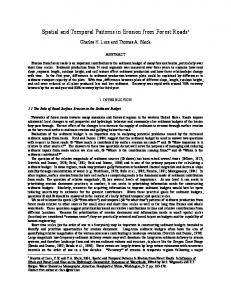
Fig. 1. Landsat scenes, ownership status, and ecoregions within the area of the Northwest Forest Plan. Forestland was determined using a method to examine the entire Landsat archive for evidence of forest presence (Yang et al. in preparation). Protected federal lands include all those where harvest is not among the management goals; unprotected federal lands are those where harvest can occur.

and culture of the PNW, with the region playing an important role in forest products nationally (Smith et al., 2009). Increasingly, however, forest conversion for urban development is becoming an important disturbance pressure (Alig & White, 2007; Kline & Alig, 2005; Kline et al., 2004). Natural disturbance agents, including wildfire and forest insect pests, play an important role in dry forests of the interior west of the U.S.(Jenkins et al., 2008), portions of which are intersected by the NWFP area. Fires are also important in the Klamath/Siskiyou ecoregion of northern California and southwestern Oregon (Staus et al., 2002), including the Biscuit Fire, which was the largest in the nation for the year 2002 (Thompson et al., 2007). 2.3. LandTrendr pre-processing, segmentation and filtering To entirely cover the NWFP area, time-series of Landsat Thematic Mapper and Enhanced Thematic Mapper Plus images (hereafter, simply “TM images”) for 22 scenes were downloaded from the USGS Glovis Website (glovis.usgs.gov) and preprocessed using methods outlined below (Fig. 1a). We refer to a “scene” as the geographic area defined for a particular path/row address in the World Reference System II [WRS-II], an “image” as one acquisition of that area by the sensor on a particular date, and the collection of images within a scene as a Landsat time-series (LTS). The goal for each LTS was to include at least one image per year for the period 1984 to 2008, although legacy data constraints resulted in occasional missing years for some scenes. Image dates were chosen to fall primarily July and August, when clouds are minimal in the region but forest vegetation is maximized. Completely cloud-free images were not required, however: in a partly cloudy year, multiple images within a given season could be chosen because the LandTrendr algorithms allow on-the-fly mosaicking (compositing) of multiple images per year. Nearly half of all images were part of these within-season, multi-image composites (Table 1). Preprocessing

of images (atmospheric correction, cloud screening, relative normalization) within each LTS followed details given in Kennedy et al. (2010), briefly summarized here. Atmospheric correction was achieved on a single reference image within each LTS using a simple COST model (Chavez, 1996). All remaining images in the LTS were normalized using the MADCAL approach (Canty et al., 2004) to match the radiometric properties of the reference image. No effort was made to normalize LTS from one scene to another. Thereafter, a cloud scoring approach was used relative to a cloud-free image in the LTS, and manual thresholding based on expert interpretation used to mask clouds and cloud shadows. For images from the ETM+ sensor after the onset of scan line errors (2003 and later), missing pixel data were also masked. The normalized, cloud-screened images in the LTS served as the foundation for subsequent processing. We defined processing footprints within each scene to provide consistency for later mosaicking and to avoid missing data caused when an individual image drifted from the idealized WRS-II location. For each scene, we calculated the Thiessen polygon (also known as a Voronoi tessellation; (Okabe et al., 2000)) delineating areas closest to the scene centerpoint. The area defined by that polygon, referred to here

Table 1 Summary of image processing efforts in Northwest Forest Plan (NWFP) area. Value Total area Total area within forest mask (forestland) Percentage of forestland in federal ownership Number of Landsat scenes processed Number of Landsat images used for mapping Images in groups >1 image per yr Median Julian day of imagery

22.99 M ha 18.5 M ha 44.2% 22 674 288 217

R.E. Kennedy et al. / Remote Sensing of Environment 122 (2012) 117–133 Table 2 Parameters used in LandTrendr processing. Process

Parameter

Value

Segmentation Spectral index Maximum number of trajectory segments Maximum p-value for fitting Recovery threshold Despiking parameter Best model proportion

Normalized burn ratioa 6 0.05 0.25 0.9 0.75

Filtering

Percent loss threshold at 1 yr Percent loss threshold at 20 yr Pre-disturbance cover threshold Percent gain threshold for growth

10 3 20 5

Mapping

Minimum mapping unit 11 pixels/ ~ 1 ha Short/long duration disturbance threshold 10 yr

a Normalized burn ratio: (Band 4 − Band 7) / (Band 4 + Band 7); See Key and Benson (2005).

121

in which case a “missing data” value was applied for that year). The time-series of these source data was then sent to the segmentation algorithms, which are controlled by a handful of parameters that affect the balance between over- and under-fitting. For this study, we chose parameters that our prior work had shown would act as a reasonable compromise in terms of error and of detection of disturbance and regrowth (Table 2). The first phase of segmentation is determination of the vertex years that define the end points of segments, and the second phase is determination of the best straight-line trajectory fit through those vertices using a flexible mix of either point-to-point or regression lines (see Kennedy et al., 2010 for details). The values returned from the segmentation algorithm are: the yearly source data (which represents the best cloud-free NBR value for that pixel in each year), the years at which vertex years were found, the fitted NBR values for those vertices, and the yearly fitted NBR data (the NBR value of each point in the segments describing the trajectory). These data were written out as separate files to be used by subsequent mapping algorithms. 2.4. Objective 1: Developing disturbance and regrowth maps

as the “Thiessen scene area”, or TSA, was considered the initial processing area for that scene. For six scenes near the margins of the study area, we manually expanded the edges of the initial TSA to avoid the need to acquire an entirely new LTS to cover a small geographic area. We then applied the LandTrendr segmentation algorithms described above to every pixel in each scene's processing area. LandTrendr algorithms operate on a single detection index; for this study, we used the normalized burn ratio (NBR), which contrasts the short-wave infrared with the near-infrared bands (NBR= (Band 4 − Band 7)/ (Band 4 + Band 7); (Key & Benson, 2005)), and which we showed previously was most responsive to disturbance in the NWFP area (Cohen et al., 2010). The segmentation process, detailed in Kennedy et al. (2010), proceeds as follows. First, image data from the LTS files were converted to NBR values and then matched on a pixel-by-pixel basis with the cloud mask. If multiple images from a given year were available, the image closest to the median date of the LTS in that scene was preferred, but if the pixel was masked, the pixel value from the image next-closest to the median was used (and repeated as necessary until a cloud free observation was available or until nor more image data were available,

2.4.1. LandTrendr disturbance mapping Disturbance maps for each scene were derived from the vertex files in several steps (Fig. 2). For each pixel, disturbance segments were defined as those showing a decline in NBR value. As described in Kennedy et al. (2010), we used a simple regression model to convert the NBR values to estimates of percent vegetative cover developed at 313 plots (r 2 = 0.75). The magnitude of disturbance for a segment was defined as the difference between the calculated vegetation cover values of the starting and ending vertices (Fig. 3a). This magnitude was divided by the pre-disturbance cover value to create a relative magnitude value truncated to ensure a range of 0 to 100%. Segments were accepted for further processing only if their relative magnitude was greater than a threshold parameter, adjusted for long versus short duration segments (see Table 2 for parameters). This filtering was shown in Kennedy et al. (2010) to be an effective means of reducing false alarms from overfitting of anomalous or ephemeral spectral features in the time-series (such as those caused by phenological variability from year to year). The duration of the

o o o

o o o

o o

o o o

Fig. 2. Work flow for developing disturbance maps from LandTrendr segmentation results. The core output of segmentation is a pair of vertex images (the year and the spectral value of vertices bounding segments). Disturbance segments are identified from these vertex images and filtered by percent cover thresholds. Adjacent pixels are grouped if they have same year of detection, and patches sorted by magnitude into a primary disturbance (Disturbance 1), a secondary disturbance (Disturbance 2), and a tertiary disturbance (Disturbance 3).

122

R.E. Kennedy et al. / Remote Sensing of Environment 122 (2012) 117–133

b

a Starting Magnitude

Duration

Ending Magnitude

d

NBR at five years c

Year of detection

Year of detection

Fig. 3. Extracting disturbance and regrowth attributes from segmented trajectories. Disturbance segments are defined as those that see a decrease in NBR over time. a) Disturbance segments lasting one year. Year of detection is defined as the first year when the disturbance can be observed, which in this case is endpoint of the disturbance segment. Both starting and ending magnitudes are converted to an estimate of percent vegetative cover, and then relative magnitude change calculated as the difference between these two values, divided by the starting magnitude. b) Disturbance segments lasting more than one year. Here, year of detection is the first year after the onset vertex. Duration is defined as the year of the ending vertex minus the year of the onset vertex. c) Change in NBR five years after disturbance (ΔNBR), used as a simple proxy for regrowth. d) As for C, but for the disturbance preceding the regrowth. The two quantities are ratioed to develop the recovery indicator.

segment was defined as the difference between the starting and ending vertex years (Fig. 3b). A given pixel could have more than one disturbance segment. Next, a magnitude file and a duration file were formed from layers recording values of the disturbance segments. Each year in the LTS stack was represented as a single layer, and data values for magnitude and duration were only present in the layer corresponding to the year of disturbance detection; remaining layers were assigned background values. We defined the year of disturbance detection as the first year after the starting vertex of the segment, since the beginning vertex of the segment necessarily predates the disturbance (Fig. 3). If the first year after the vertex was masked out because of clouds or gaps from the scan-line correction error in ETM + data, the next valid year was used instead. After creating yearly magnitude and duration files, minimum mapping unit rules were applied to ensure that patches of disturbance were at least 11 pixels (approximately 1 ha) in size. This size was small enough to easily capture most timber management activities in the region, but large enough to avoid mapping disturbance events that are too small to easily validate over the large mapping domain. First, adjacent pixels in a given year (layer) were grouped together into patches using an eight-neighbor rule, and each group was assigned a unique identifier. To avoid grouping pixels in clearcuts with those from long-duration processes that happen to begin in the same year (such as those caused by insects), disturbances with durations greater and less than 10 years were grouped separately within a given layer. Because the co-occurrence of these phenomena is very rare, the choice of 10 years was based on conservative comparison with insect events interpreted using the TimeSync tool (Cohen et al., 2010). After group membership was defined for all pixels, any groups with fewer than 11 pixels were identified and removed by setting all member pixels to the background value. For remaining patches, gaps smaller than 11 pixels were filled if they were adjacent to three non-background pixels using a 4-neighbor rule (cardinal directions). This gap filling was applied iteratively three times. In each iteration, the median of the surrounding pixels was used to assign values to the filled pixels (rounded to integer value for duration); these were then added to the patches. Finally, disturbance maps for each scene were created from the yearly magnitude and duration images. These maps had three layers of information: year of disturbance detection, relative magnitude of disturbance, and duration of disturbance. Where a given area experienced more than one disturbance in the LTS, we first sorted

disturbance patches according to the sum of the patch area × relative magnitude value, providing balance between large, low-magnitude and small, high-magnitude events. The highest-scoring patch in a given area was placed in a “primary disturbance” map and the nexthighest in a “secondary disturbance.” We also developed maps of “tertiary disturbance,” but these were extremely rare and thus were ignored for the remainder of this study. The final disturbance map was created by mosaicking all scenes together and applying a non-forest mask. Mosaicking of scenes occurred in a sequential order of rows within a path and then of adjacent paths. In the overlap area between any two scenes, the scene later in the order overrode the earlier one. No effort to normalize or standardize map products across scenes was conducted. Separately, we developed a mask to define where forest existed at any point in the observation record. To develop this mask, we first applied the second phase of segmentation (fitting) to tasseled-cap (TC) brightness, greenness and wetness (Crist & Cicone, 1984) images in the LTS, using the vertex years derived from the NBR-based segmentation, resulting an LTS of fitted TC values. We then calculated the tasseled-cap angle (TCA) index (Gómez et al., 2011; Powell et al., 2010) for each year in each pixel's time series. Because higher TCA values correspond to higher forest cover, we selected the segment with the highest average TCA as the time period in that pixel's history that was most “forest like.” We then recorded the mean and mean-square-error of the fitted TC brightness, greenness, and wetness values for that segment. Finally, this image was used in a statistical random-forest classification (Breiman, 2001) trained from polygons of forest delineated using expert interpretation across the NWFP area. Pixels identified as forest in this mask were thus those that appeared forest like at any point in the entire time period (1984 to 2008). The final disturbance map was filtered to remove any disturbances mapped in non-forest pixels. 2.4.2. LandTrendr regrowth mapping To map post-disturbance regrowth, two metrics of vegetative recovery were calculated, one absolute and one relative (Fig. 3). The absolute measure was referred to as the post-disturbance regrowth, and represented the change in NBR at five years after disturbance, calculated as: ΔNBRregrowth ¼ NBRf itted;t5 −NBRf itted;t0 where NBRfitted, t5 and NBRfitted, t0 correspond to the NBR from the fitted time series five years after disturbance and for the vertex defining the

R.E. Kennedy et al. / Remote Sensing of Environment 122 (2012) 117–133

123

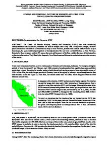
Fig. 4. Primary disturbance maps for the area of the NWFP. Year of disturbance detection, relative percent vegetation loss, and disturbance duration are calculated for all pixels in the study area. Large fires are evident throughout the study area, particularly in southern Oregon and in California. Harvest is widespread throughout the region. Note that non-forest areas have been masked out.

beginning of the regrowth segment (and, by definition, the endpoint of the disturbance segment). The second index scaled the postdisturbance regrowth value to the loss of vegetation in the preceding disturbance. Referred to as the “recovery indicator,” it was calculated as: RI ¼

ΔNBRregrowth ΔNBRdisturbance

where the denominator is change in NBR during the disturbance segment that precedes the regrowth. By scaling, the recovery indicator

compensates for forests that begin at lower NBR and for lower magnitude disturbances that leave more residual NBR. 2.4.3. Map accuracy We assessed the accuracy of the map using the TimeSync interpretation tool (Cohen et al., 2010) applied 2360 at randomly-chosen points across the entire NWFP area. Plots were distributed with an approximate goal of 200 per full Landsat scene (with many partial scenes receiving fewer than 200). A three-by-three pixel area

124

R.E. Kennedy et al. / Remote Sensing of Environment 122 (2012) 117–133

Table 3 Summary of TimeSync interpretation efforts in the NWFP area. Property

Value

Number of randomly-selected interpretation plots Number of plots falling in foresta Number of plots showing evidence of disturbance Number of plots showing greater than one disturbance Number of disturbance events, by type: Harvest Fire Insect Other

2360 2136 778 249

a

740 192 50 96

A plot is counted if at least one of its nine pixels intersects the forest mask.

we stratified plots by TimeSync magnitude and agent and by relative magnitude recorded by LandTrendr (median magnitudes greater than 66%, between 33 and 66%, and less than 33% for high, medium and low classes). Additionally, we tallied plots separately depending on whether the interpreter noted that the disturbance occurred on either greater than or less than five of the nine pixels. There was no separate assessment of regrowth maps. Because regrowth segments are tied to their preceding disturbance segments in both LandTrendr and TimeSync, the presence or absence of regrowth in our maps would adhere to the accuracies calculated for the associated disturbances, making a separate accuracy assessment redundant. 2.5. Objective 2: Evaluate monitoring questions

centered on each plot was evaluated, and for each disturbance segment we recorded the relative magnitude of the disturbance (High, Medium, or Low), the cause of the disturbance (Fire, Harvest, other), and the number of pixels within the three by three window affected (1 through 9 pixels). Table 3 summarizes the characteristics of the interpreted plots. We emphasize that these plots were chosen independent of the disturbance maps. We then linked the database of interpretation to the primary disturbance map. From the disturbance map we extracted the pixels in the three-by-three window used for TimeSync interpretation for all plots. If any of the nine pixels were within one year of a disturbance segment defined by the interpreter for the plot, we recorded a match. We then calculated the median magnitude of all pixels mapped as disturbed within the plot window. To construct an agreement tables,

The maps made using methods described in Section 2.4 provided the raw material by which the monitoring questions described in Section 1 were evaluated. The disturbance maps were intersected with ownership and ecoregion maps, and then summarized yearly within geographic strata by the area, magnitude, and duration of disturbed pixels within those strata. To allow comparison across strata of different sizes, areas were also scaled to total area by type to estimate proportion of land ownership disturbed by year. Regrowth maps were intersected with ecoregion and ownership maps. Histograms of area in each regrowth NBR and RI bin were summarized by ecoregion and ownership category. Ownership layers were derived from Protected Areas Database of the United States Version 1.1 (USGS GAP analysis program; gapanalysis.usgs.gov/data/padus-data/). Ecoregion maps

Fig. 5. Primary and secondary disturbance maps at local scales. Relative magnitude (a), year (b), and duration (c) of disturbance for an area including Mt. Rainier National Park (inset box on Fig. 4a). Background on (a) is a high resolution airphoto and on (b) a topographically shaded elevation model, with ownership boundaries displayed as gray lines. Parts (d) and (e) show primary and secondary disturbance, respectively, for a very local scale on private forest land just west of the areas in parts (a)–(c). Secondary disturbances often corresponded to activities preceding harvest, such as road-building, although occasionally also detected two episodes of harvest.

R.E. Kennedy et al. / Remote Sensing of Environment 122 (2012) 117–133

were obtained from the US Environmental Protection Agency (Level III Ecoregions, published 2003).

Table 5 Summary of primary disturbance mapped in the NWFP area. State

Ownership

Total area disturbed 1985–2008 (in hectares)

Area disturbed as a percentage of forest area within ownership

Washington

Federal, protected Federal, non-protected Private State Native Other

110,111 240,613 1,061,148 238,036 126,107 20,901

9.0 14.3 39.7 28.7 36.9 19.5

Oregon

Federal, protected Federal, non-protected Private State Native Other

139,396 578,565 1,210,072 66,315 43,770 1277

23.5 18.6 39.6 19.8 39.2 14.8

California

Federal, protected Federal, non-protected Private State Native Other

168,925 347,241 501,368 21,071 8888 4821

27.9 20.6 22.3 19.9 12.4 15.2

3. Results 3.1. Objective 1. Mapping We recorded a total of 4.9 M ha of primary disturbance in forests within the NWFP area over the period 1985 to 2008 (Fig. 4), including a range of detection year, magnitude, and duration values (examples in Fig. 5a–c). Comparison with point-based interpretation from TimeSync showed expected patterns of agreement of LandTrendr map products. Considering only plots where the majority of pixels were affected (five or more of the nine possible), disturbance detection was highly successful for both high and medium disturbance, and even moderately successful for low-intensity disturbance (Table 4). We compared agreement before and after forest mask application; no substantial changes in errors of omission were noted (data not shown). False detections by the algorithm (“No Disturbance” column in Table 4) only occurred when four or fewer pixels were considered, and then primarily for low magnitude detections. Because the TimeSync tool allows an expert interpreter to compensate for false spectral changes caused by phenological or atmospheric effects in individual years, agreement between TimeSync results and the LandTrendr algorithms confirms that the algorithms were robust to such ephemeral noise, as intended in the design of the segmentation approach. Of the abrupt disturbances, secondary disturbances covered an area less than 5% of the area covered by primary disturbances. Maps of secondary disturbance revealed events such as road-building preceding a harvest and lower-magnitude harvest events before or after the main harvest event (Fig. 5d and e). Because of the low frequency of secondary disturbance and because most disturbances appeared related to the primary disturbance, we used only primary disturbances to evaluate the core monitoring questions above. 3.2. Objective 2: Evaluating monitoring questions 3.2.1. How does aggregate disturbance vary across owner categories, states, and ecoregions? Forest disturbance area varied by owner and state. For the entire period from 1985 to 2008, the proportion of each ownership type's forest area experiencing primary disturbance ranged from a low of 9.0% on protected federal lands in Washington to high values exceeding 36% on private and native lands in both Washington and Oregon (Table 5). The latter values are equivalent to yearly rates of more than 1.5%. In California, however, proportional areas disturbed on private and native lands were much lower than the other states, but proportional forest disturbance on federal lands was higher.

125

Of the primary disturbances mapped, most were abrupt (lasting 1, 2, or 3 years), but on protected lands more than a quarter of the area mapped as primary disturbance showed duration greater than 15 years (Table 6). Although such long-duration disturbance signals can be associated with forest insect activity (Goodwin et al., 2010; Meigs et al., 2011; Vogelmann et al., 2009). Attribution of change is beyond the scope of the current study. Therefore, to constrain analysis to better-defined disturbance, we focus all further analysis on abrupt disturbance events. Total forest disturbance (primary, abrupt) within the NWFP area varied by ecoregion and state (Fig. 6). Comparing the four larger ecoregions that span two or three states, several notable patterns emerged. Disturbance in the Coast Range province predominantly occurred on private lands in all three states, suggesting that federal policies would have limited leverage to affect overall forest disturbance condition. The Cascades province contains significant forest area in both Washington and Oregon, but in Washington the disturbance predominantly occurred on private lands while in Oregon it was balanced between private lands and federal, non-protected lands. Although the East Cascade Slope occupies relatively little forest area within the NWFP, the ecoregion was unusual in having relatively high proportional disturbance on tribal lands in both Washington and Oregon. The Klamath ecoregion was also unusual in having relatively high proportions of forest disturbance that occur on protected federal lands (predominantly fire).

Table 4 Agreement of disturbance maps with human-interpreted disturbance calls, grouped by human-labeled agent and magnitude, LandTrendr magnitude, and tallied separately for plots where greater and less than five of nine pixels were affected (as defined by the interpreter). TimeSync interpretation High

Higha Medium Low No Disturbance Producer's Accuracy Landtrendr

a

Medium

Low

Fire

Harvest

Other

Fire

Harvest

Other

Fire

Harvest

Other

No disturbance

35/0b 20/0 0 5/0 0.92c

62/0 36/1 0 9/0 0.92

4/1 0 0 1/0 0.80

0 23/0 5/1 4/0 0.88

20/2 129/8 28/0 29/2 0.86

0/1 10/0 2/0 12/2 0.50

1/1 4/4 14/10 9/6 0.68

2/9 31/41 63/44 65/115 0.60

2/0 6/2 11/0 35/18 0.35

0/20 0/60 0/224

High: >66% relative change; Medium: between 33 and 66% relative change; Low: >33% relative change. Within each table cell, reporting format is: # of plots where 5 or more pixels were affected/# of plots where 4 or fewer pixels were affected, in both cases determined by the human interpreter. c Producer's accuracy only calculated using scores for >5 pixels. b

126

R.E. Kennedy et al. / Remote Sensing of Environment 122 (2012) 117–133

Table 6 Abrupt versus long duration disturbance by protection status for primary disturbance. Disturbance duration by protection status Protection status

Percentage with duration b 4 yr

Percentage with duration between 4 and 15 yr

Percentage with duration > 15 yr

Protected Non-protected

69.7 84.2

6.5 5.6

30.4 10.2

3.2.2. Across the entire NWFP area, how did disturbance rate on federal lands change during court injunctions and subsequent implementation of the NWFP? Addressing the second monitoring question requires disaggregation of disturbance by year (Fig. 7). The area of forest land experiencing abrupt, primary disturbance was relatively consistent across most years, with some notable exceptions in 1988 and 2003. (Fig. 7a). Based on analysis of data from the Monitoring Trends in Burn Severity

Washington

Area

Oregon

Proportion of Disturbance

Area

Proportion of Disturbance

California

Area

Proportion of Disturbance

ha

Coast Range

a

(MTBS) project (mtbs.gov; data downloaded February 2011), 1987 and 2002 were years where fires burned more than 13 times the median area in the three states. Because most images in the LTSs were acquired in mid-summer (median Julian date 217), fires occurring in the late summer and early fall would first be detected in our maps in the following year (i.e. 1988 and 2003). Cumulative disturbance area provides insight into the rates of harvest (disturbance/year, represented by the slope of the cumulative disturbance curve) and when those rates changed (Fig. 7b). From 1985 through the late 1990s, federal lands were disturbed at rates similar to private and tribal lands (as indicated by similar slopes of disturbance accumulation), but beginning in 1990, disturbance rates on federal, non-protected lands slowed considerably. This coincides with the time that court injunctions halted most harvest on federal lands (USDA & USDI, 1994). Notably, the rate of forest disturbance did not appear to return to pre-injunction levels when the NWFP was implemented in the early to mid 1990s.

State Native

Not Disturbed Disturbed

Private Fed. Unprot.

Fed. Prot. Other

ha

Cascades

b

ha

East Cascade Slope

c

ha

Klamath Mtn

d

Fig. 6. Total disturbance (primary, abrupt) distributed by state and ecoregion. Bar charts show total forest area and the area disturbed, while pie charts show the proportional allocation of disturbance among owner categories. Shown are the four ecoregions that intersect two or three of the states in the study: a) Coast Range, b) Cascades, c) East Cascade Slope and d) Klamath Mountain. Note the dominance of private land disturbance across ecoregions, particularly the Coast Range province, as well as the variability among states in the distribution of disturbance across different owner categories.

a

a

30

3500

2000

10

1500

15

Proportion (%)

2500

20

25

3000

Area (100ha)

127

35

R.E. Kennedy et al. / Remote Sensing of Environment 122 (2012) 117–133

5

1000

0

500

b

c

35

Year of Detection

1985 1986 1987 1988 1989 1990 1991 1992 1993 1994 1995 1996 1997 1998 1999 2000 2001 2002 2003 2004 2005 2006 2007 2008

1985 1986 1987 1988 1989 1990 1991 1992 1993 1994 1995 1996 1997 1998 1999 2000 2001 2002 2003 2004 2005 2006 2007 2008

1985 1986 1987 1988 1989 1990 1991 1992 1993 1994 1995 1996 1997 1998 1999 2000 2001 2002 2003 2004 2005 2006 2007 2008

0

20 10

15

20 15

3.2.4. Do the answers to questions 2 or 3 vary by state? Separating cumulative rates by state reveals further contrast both among ownerships and among states (Fig. 8). Overall rates of disturbance (slope of the line of disturbance area by time) were highest in Washington and Oregon, and within those two states both private and native lands showed high rates relative to other ownerships.

25 20 15

Proportion (%)

1985 1986 1987 1988 1989 1990 1991 1992 1993 1994 1995 1996 1997 1998 1999 2000 2001 2002 2003 2004 2005 2006 2007 2008

0

3.2.3. Did disturbance rate on non-federal lands change in response to the change on federal lands? Rates of forest disturbance on private lands and on lands classified as “other” (typically municipalities and small government holdings) were relatively consistent over the entire period (Fig. 7b), showing no compensatory increase after 1990 as harvest on federal lands decreased. However, rates on native lands did begin to increase through the mid 1990s, such that native lands eventually surpassed state lands in cumulative proportion disturbed. Interestingly, disturbance rates on state-administered lands declined in the early 1990s although not affected directly by the federal court rulings, but then returned to rates similar to those on private lands by the 2000s. Rates on protected federal forest land were very low, but showed periodic step-function type increases, particularly in 1988, 2000, 2003 and 2007 that moved the cumulative forest disturbance area by the end of the recording period to a level more than half that on federal non-protected lands.

5

10

Fig. 7. Abrupt (b 4 year duration), primary disturbance for the NWFP area. a) Yearly disturbed area by ownership category. b) Cumulative proportions of forest disturbance by ownership. The slope of the cumulative proportion charts indicates rate of disturbance. Rates were highest on private lands, followed closely by native and state lands. Protected federal lands experienced occasional, large disturbances.

30

Year of Detection

35

0

1985 1986 1987 1988 1989 1990 1991 1992 1993 1994 1995 1996 1997 1998 1999 2000 2001 2002 2003 2004 2005 2006 2007 2008

0

5

5

10

Proportion (%)

25

Proportion (%)

25

30

30

35

b

Fig. 8. Cumulative forest disturbance rates as in Fig. 7b, but stratified by state. Washington (a) and Oregon (b) were similar in having high rates of disturbance on private lands and native lands, but differed in the rates on state-owned lands. Federal lands in Oregon experienced marked diminishment in rate after federal harvest injunctions in 1991. Oregon and California (c) showed dramatic increases in disturbance on protected federal lands, associated with large fire events.

The increase in disturbance rate on native lands after 1993 was particularly noticeable in Washington. Lands administered by the state in Washington tracked the high rates on private lands until approximately 1992, when the rate slowed. In Oregon, rates on state lands were low until the late 1990s, when the yearly disturbance increased to make the rate of disturbance similar to that on private lands in the state. The impact of court injunctions was particularly noticeable in Oregon, where the rate of disturbance on federal non-protected lands slowed after 1990. Protected federal forestlands showed dramatic increases in disturbance area in both Oregon and California in high fire years (1987–1988, 1999–2000, 2002–2003, and 2007–2008),

128

R.E. Kennedy et al. / Remote Sensing of Environment 122 (2012) 117–133

condition (NBR five years after disturbance) was highest in moist and temperate ecoregions (Cascades, Coast Range, and Puget Lowlands) and lowest in drier ecoregions (California Chaparral and Oak woodland, East Cascade Slope; Fig. 10a). Ecoregions containing a mix of dry and moist conditions showed a broad range of NBR values (North Cascade and Willamette Valley). When vegetative recovery five years after disturbance was compared to NBR loss during disturbance (recovery indicator, Fig. 10b), variability among most ecoregions diminished, and two drier ecoregions emerged as having particularly low recovery rates (East Cascade Slope and Klamath Mountain). Within ecoregions, vegetative recovery rates varied by owner category and state. For the four ecoregions that spanned two or three states in several owner categories, we rendered distributions of the recovery indicator values as heatmaps, with lighter tones corresponding to greater counts in the distribution (Fig. 11). Although rates are quite diverse, several themes emerged. Vegetative regrowth rates did vary by state, suggesting that state-level policy constraints could be having an effect. However, the relative direction of effect across states was not consistent: For example, on private lands in the Coast Range and Cascades ecoregions, vegetative regrowth rates were highest in Washington and lowest in California, but in the East Cascades

such that protected federal lands in both states ended with cumulative disturbed areas nearly as high as those on the non-protected federal lands. 3.2.5. Did disturbance intensity on federal lands decrease as the NWFP was implemented? Disturbance magnitude on private and on non-protected federal lands show similar distributions through the 1980s and early 1990s, but beginning the mid-1990s magnitudes of disturbance on federal lands declined substantially and remained lower than those on private lands through the period of record (Fig. 9). We emphasize that these magnitudes are based on a spectral model of vegetative cover, not strictly forest cover, and that therefore they cannot be interpreted directly as estimates of tree canopy loss. Nevertheless, they imply a change in the type of disturbance on federal lands that was not matched on private lands for the same period. 3.2.6. Did post-disturbance vegetation recovery vary by ecoregion, ownership category, or state? Area histograms of absolute and relative recovery indicators were calculated by ecoregion (Fig. 10). Absolute post-disturbance vegetation 1985

1986

1987

1988

1989

1990

1991

1992

1993

1994

1995

1996

1997

1998

1999

2000

2001

2002

2003

2004

2005

2006

2007

2008

100 80 60 40 20

Disturbance Magnitude

100 80 60 40 20

100 80 60 40 20

100 80 60 40 20

100 80 60 40 20

100 80 60 40 20 0

1

2

3

4

0

1

2

3

4

0

1

2

3

4

0

1

% Fig. 9. Changing magnitude of abrupt, primary disturbance on federal and private lands within the NWFP area. The x-axis corresponds to the percentage of each year's disturbance in disturbance magnitude categories on the y-axis. Private and federal lands had similar magnitudes of disturbance through the 1980s, but federal lands began to drop in magnitude after the mid 1990s as NWFP management actions were implemented.

R.E. Kennedy et al. / Remote Sensing of Environment 122 (2012) 117–133

129

a 1.2 1.0

%

0.8 0.6 0.4 0.2 0.0

0.05

0.10

0.15

0.20

NBR

b 2.0

%

1.5

1.0

0.5

0

20

40 60 Recovery Indicator

80

100

Fig. 10. Post-disturbance vegetation regrowth as measured by two spectral metrics. a) Proportion of total area at different levels of absolute NBR at five years after disturbance, stratified by ecoregion. b) As for a), but for the recovery indicator (RI, see Fig. 3a). Dry ecoregions showed lower absolute NBR and lower recovery indicator rates, indicating slower regrowth of vegetation after disturbance.

ecoregion, the order was essentially reversed. Protected lands generally showed lower vegetative recovery rates, except in the case of Oregon's Klamath ecoregion. Finally, variability among state and owner categories was lower in the wettest and driest ecoregions (Coast Range and East Cascade Slope, respectively) than in the intermediate ecoregions (Cascades and Klamath).

segmentation approach complements other time-series approaches by detecting both trends and abrupt deviations with a consistent methodology. The underlying goal of the current study was to move the temporal segmentation strategy toward large-area mapping in support of forest monitoring. 4.1. Challenges in large-area mapping

4. Discussion Widespread modification of the land surface may have important consequences for human and natural systems (DeFries et al., 2004; Ramankutty et al., 2006), and satellite-based monitoring will necessarily be central to understanding those consequences and measuring effectiveness of responses (Turner et al., 2007). Although the information content of the Landsat data archive is appropriate to track diverse land change processes, its very richness poses a challenge for concise description and mapping. With open access to consistent data and with increasingly affordable data manipulation and storage capabilities, however, many approaches are emerging to use timeseries Landsat imagery to meet this challenge (Gómez et al., 2011; Goodwin et al., 2010; Hais et al., 2009; Helmer et al., 2010; Huang et al., 2010; Masek & Collatz, 2006; Olsson, 2009; Powell et al., 2010; Röder et al., 2008; Schroeder et al., 2011; Vogelmann et al., 2009), including the LandTrendr and TimeSync tools used here. All of these methods build on earlier studies of multi-date Landsat imagery to either characterize trends in the spectral signal over time (Hostert et al., 2003a; Lawrence & Ripple, 1999; Viedma et al., 1997) or abrupt deviations from normative conditions (Almeida & Shimabukuro, 2002; Cohen et al., 2002; Hayes & Sader, 2001; Jin & Sader, 2005; Sader et al., 2003). Free access to data has also led to emergence of new approaches to map large geographic areas at relatively coarse temporal resolution (Hansen et al., 2010; Masek et al., 2008; Potapov et al., 2009; Roy et al., 2010). The LandTrendr temporal

The methods to derive maps from time-series segmentation represent a first effort that can be improved in several key areas. First, although the LandTrendr algorithm can mosaic multiple partly-cloud images within a given year to minimize data gaps, some areas in some years cannot be viewed because of persistent clouds or Landsat 7 data gaps. When a disturbance occurs in those areas in the year of the missing data, the disturbance first appears in the record the year after (or, depending on further data gaps, multiple years after) the actual disturbance, diminishing the disturbance count in the year with gaps and inflating the count in the subsequent year. At the geographic scale at which results are reported here, this problem is minor, but when annual disturbance maps are used at the local scale for monitoring or modeling purposes, some means of distributing disturbances into data-gap periods will be necessary. Second, rules for spatial aggregation and filtering are challenging to define for time-series data. The premise of such filtering is that disturbances occur and are detected as spatially-coherent patches that appear on the landscape at a single point in time, but this is not always the case. Long-duration processes of both mortality and growth emerge slowly and often spread across the landscape, making strict rules for simultaneity too restrictive for determining which pixels belong together. Even events that do appear at the same time may not always be detected in the same year, in part because of data gaps (as described above) and in part because of imprecise segmentation caused by chance fluctuation of a pixel's signal in the year

130

R.E. Kennedy et al. / Remote Sensing of Environment 122 (2012) 117–133

a

b

c

d

Fig. 11. Distributions of recovery indicator values as in Fig. 10b, but shown as heat-maps to allow comparison among owner categories across states. Lighter tones correspond to greater density in the distribution of recovery indicator values (corresponding to local peaks in the distributions in Fig. 10). Shown are the four ecoregions that are also shown in Fig. 6: a) Coast Range, b) Cascades, c) Klamath Mountains, d) East Cascade Slope.

before or after an abrupt event. In either case, rules that allowed adjacent pixels to be slightly mismatched may help, but these in turn could cause false agglomeration of adjacent disturbances that were indeed in separate years. A similar concern arises with the gap-filling strategy, which at present assumes that small gaps surrounded by disturbance must be false omissions. Strict adjacency rules often introduce these gaps, making the gap-filling a legitimate approach in many situations, but for patchy phenomena it may falsely ascribe change where none occurred. Eventually, better rules to assign pixels to patches may need to consider a combination of spatial and spectral neighborhood, perhaps in conjunction with training datasets tuned to a particular landscape. Evaluating the accuracy of maps based on time-series data is also challenging. The TimeSync interpretation tool eases this process in two important ways. First, by producing a manual analog to the

automated temporal segmentation, it allows logically consistent comparison between algorithm and interpreter. Second, it allows description of change processes more robustly than in the past (Cohen et al., 2010), allowing rich interpretation of map robustness according to agent, severity, and size of disturbance (Table 5). Challenges remain, however. To account for slight geographic misregistration, TimeSync interpretation is conducted for a three-by-three window that must be resolved to compare with map products. A related challenge concerns point-based validation of patch-based maps. While the point-based approach facilitates a randomized sample that is untethered to any particular map, it introduces an area bias into accuracy assessment. Because a random sample is more likely to land in a large patch than a small one, detection of false omissions is a function of patch size or spatial frequency: the omission or inclusion of a high-spatial-frequency pattern is difficult to detect with a point-based sample. Other alternatives for

R.E. Kennedy et al. / Remote Sensing of Environment 122 (2012) 117–133

sampling validation do exist (Congalton & Green, 1999; Thompson, 2002), but no single approach is likely to meet all challenges. Another challenge in validation lies in the construction of maps reporting yearly disturbance. A key cell in the confusion matrix is conceptually problematic: the agreement between the interpreter and the algorithm on the absence of disturbance (the lower righthand cell in Table 5). Because a disturbance could occur in any year, agreement could be tallied for all years in the time-series where the algorithm agrees with the interpreter that no disturbance occurred, and in evaluation of time-series segmentation alone this approach can be used to calculate algorithm accuracy (Cohen et al., 2010). In a map context, however, it would imply the existence of a disturbance map for each year, which is not consistent with the character of the final disturbance map. Thus, for this study we focused on class-byclass agreement, and do not attempt to compress the entire map into a single accuracy or kappa statistic (Congalton & Green, 1999). Finally, our approach to mapping regrowth is nascent. The current approach reflects a common strategy used in regrowth mapping efforts, where regrowth is expressed in relative terms scaled by the degree of change in spectral index over time (Gómez et al., 2011; Hostert et al., 2003b; Schroeder et al., 2007; Viedma et al., 1997). In our study, the model of vegetative cover based on the NBR index is relatively robust, and thus we believe that the use of the index to track vegetative change is largely justified. However, most models of percent cover or of land cover type are based on training data collected primarily in undisturbed conditions; it is unclear whether the identical spectral properties before and after disturbance may correspond to entirely different conditions on the ground. Regardless, it is likely that a single spectral index will be insufficient to adequately characterize recovery, and it may also be necessary to develop separate models linking spectral properties to post-disturbance conditions. Finally, labor-intensive validation of point-in-time estimates of regrowth would be necessary to completely validate the full range of regrowth rate estimates. Mosaicking of maps was easier than expected. With no effort to calibrate across the 22 scenes used for mapping, the resultant maps of disturbance showed relatively few scene boundary artifacts. The temporal segmentation process largely removes within-scene artifacts of phenology, sun-angle, and atmospheric effects that typically introduce scene boundaries, apparently to the degree that little cross-scene calibration may be needed. 4.2. Matching maps with land change processes Despite the many challenges introduced in large-area mapping of segmentation algorithm outputs, the potential information content of the resultant maps has utility for monitoring change processes on the landscape. For example, by capturing long-duration processes, we can show that protected forests experience a much higher proportion of chronic disturbance than do non-protected forests (Table 6). By detecting changes in the magnitude of disturbance over time, we can infer changes in forest harvest type (thinning vs. clearcut) that are consistent with intended policy goals (Fig. 9). The annual information content provided by the time-series approach is commensurate with policy changes, allowing better interpretation of the likely causes of disturbance over time (Figs. 7–9). By tracking both disturbance and regrowth with the same measurement tool, we are able to derive metrics of regrowth relative to disturbance in a manner that would be less consistent if attempted from different sources (Figs. 10 & 11). 4.3. Monitoring results In addressing the core monitoring questions, several key themes deserve note. First, the NWFP appears to have affected forest disturbance rate in ways intended by the policy: Rates of disturbance on federal lands were lower under the NWFP than before the court

131

injunctions in the late 1990s, and when harvest did occur, it was lower in severity than before the NWFP. This analysis complements and extends analyses in the region that pre-date the NWFP (Cohen et al., 2002; Spies et al., 1994; Turner et al., 1996). Lower rates of disturbance are consistent with observations of timber production estimated from mill production (Raettig & Christensen, 1999). But rates of harvest on federal lands were proportionally much lower than on most other owner categories (Fig. 7), meaning that the NWFP has limited ability to control overall disturbance rate on the landscape. Second, tribal lands, particularly in Washington state, appear to be the only owner category where disturbance rates increased after implementation of the NWFP lowered rates on federal lands; disturbance rates on private lands were remarkably constant across years (Figs. 7 and 8). Third, disturbance on protected federal lands had the lowest rates of all owner categories, as expected, but showed relatively high rates of long-duration disturbance (Table 6), presumably associated with chronic mortality or stress, such as that caused by insects. Similarly, protected federal lands also experienced sharp spikes in disturbed area because of fires. Together, these results emphasize that the ability of the federal policy to control disturbance is constrained not only by the presence of many other owner categories, but also by natural processes that are unlikely to be affected by policy. Fourth, rates of disturbance on state-controlled lands varied over time. Harvest on state lands was high in Washington, but began to decrease at approximately the same time as the enactment of the NWFP, perhaps in response to general concerns about management for endangered species evoked by the court injunctions leading to the NWFP. Investigating the Washington forest practices act (www. wfpa.org), we found no official amendment in forest regulation to explain this change. In contrast, Oregon's state forest practice act was amended in both 1991 and 1994 to increase regulation of forest harvest, and our data suggest a subtle decrease in disturbance rate in the early 1990s. Despite these changes, area of disturbance increased on Oregon's state forest lands in the mid 1990s to early 2000s, a period when rates of harvest in two of Oregon's larger state forest increased (Oregon Department of Forestry Timber Harvest Reports; http://www. oregon.gov/ODF/STATE_FORESTS/FRP/annual_reports.shtml). In contrast to Oregon and Washington, rates of harvest on state lands in California were among the lowest by ownership class. Comparisons across states are difficult from state records alone, as reporting metrics vary and data quality is likely differential both across time and states. Satellite-based measurements provide a consistent tool to facilitate a level comparison. Finally, the patterns of vegetative regrowth varied by state and ecoregion in both expected and unexpected ways. Drier ecoregions showed slower regrowth rates, reflecting the expected reduction in vegetative vigor under water limitation. When evaluated within ecoregions, state-level effects were generally unexpected. Rules for “greenup” (ensuring post-harvest establishment of forest) on private and state lands are generally similar among the three states, but considered somewhat more restrictive in California (Boston & Bettinger, 2006). Yet our metric for post-disturbance regrowth (RI, recovery indicator) indicated that regrowth was slower on private and state lands in California than on similar lands in Washington and Oregon for the Coast Range and Cascades ecoregions (Fig. 11a and b). Although this pattern could be caused by generally drier conditions in California for any given ecoregion, that thesis is weakened by noting that the state-level effect did not appear on federal non-protected lands. Clearly, the satellite signal may have useful information to compare forest practices across states, but the patterns will require considerably more interpretation based on site-specific knowledge of actual forest management practices. We also emphasize that our recovery metric, based on the response of a single spectral index five years after disturbance, is only related to vegetative regrowth,

132

R.E. Kennedy et al. / Remote Sensing of Environment 122 (2012) 117–133

not tree regrowth, and does not necessarily serve as a proxy for ecological health or integrity. 4.4. Applicability to other land change topics Although developed with the intent of monitoring land change in forests of the Pacific Northwest, U.S., the algorithms and map-making steps described in this study are technically generic and could be applied to any system, given two overarching constraints: 1) Data density must be high enough to allow for description of the timeseries as a trend, not as a series of disjunct snapshots, and 2) Spectral stability must be high enough that targeted change processes cause spectral change durable enough to be distinguished from year-toyear noise. The former constraint can be difficult to meet if the Landsat archive is temporally sparse (typical outside the contiguous 48 states) and/or cloudy. While LandTrendr can work with multiple cloud images per year, individual pixels must have a clear view often enough to provide useful time-series. Although we have not yet rigorously tested boundaries of either constraint, a rule of thumb is that at least 10 to 12 useful data points are needed to delineate a classic trajectory of stability followed by disturbance and then regrowth. Beyond mere technical applicability in other systems, the LandTrendr approaches also have practical applicability. We currently use the described approaches in other ecosystems of the western U.S., as well as in eastern European countries. The general assumptions of the method appear consistent across ecosystems: Given a spectral index appropriate for the ecosystem, a relationship between that variable and some metric of vegetation density, and a disturbance regime characterized by temporally consistent patch effects, the LandTrendr mapping approach is useful. Moreover, by utilizing many examples of stability in each pixel, deviation from that stable background signal is more easily detected at lower thresholds (Cohen et al., 2010), suggesting that overall signal to noise ratio for any land cover separation question would benefit from the approach. 4.5. Summary Taken together, these results underscore how the depth (Wulder et al., 2008) and free-data access policy of the Landsat archive (Woodcock et al., 2008) improve our ability to map landscape processes in forests. Through their temporal and spatial consistency, these data contain information on abrupt, stochastic events and on trends. With appropriately defined algorithms (Kennedy et al., 2010), we can simultaneously map these contrasting phenomena, both to document expected changes and to reveal potentially new patterns or processes occurring on the landscape. By addressing these monitoring questions, the mapping approaches documented here provide the raw material on which investigations of drivers could be based. Acknowledgments The development and testing of the LandTrendr algorithms reported in this paper were made possible with support of the USDA Forest Service Northwest Forest Plan Effectiveness Monitoring Program, the North American Carbon Program through grants from NASA's Terrestrial Ecology, Carbon Cycle Science, and Applied Sciences Programs, the NASA New Investigator Program, the Office of Science (BER) of the U.S. Department of Energy, and the following Inventory and Monitoring networks of the National Park Service: Southwest Alaska, Sierra Nevada, Northern Colorado Plateau, and Southern Colorado Plateau. References Alig, R., & White, E. (2007). Projections of forestland and developed land area in western Washington. Western Journal of Applied Forestry, 22, 29–35.

Almeida, R., & Shimabukuro, Y. E. (2002). Digital processing of a Landsat-TM time series for mapping and monitoring degraded areas caused by independent gold miners, Roraima State, Brazilian Amazon. Remote Sensing of Environment, 79, 42–50. Beach, R. H., Pattanayak, S. K., Yang, J. -C., Murray, B. C., & Abt, R. C. (2005). Econometric studies of non-industrial private forest management: A review and synthesis. Forest Policy and Economics, 7, 261–281. Boston, K., & Bettinger, P. (2006). An economic and landscape evaluation of the greenup rules for California, Oregon, and Washington (USA). Forest Policy and Economics, 8, 251–266. Breiman, L. (2001). Random forests. Machine Learning, 45, 5–32. Canty, M. J., Nielsen, A. A., & Schmidt, M. (2004). Automatic radiometric normalization of multitemporal satellite imagery. Remote Sensing of Environment, 91, 441–451. Chavez, P. S., Jr. (1996). Image-based atmospheric corrections — Revisited and improved. Photogrammetric Engineering and Remote Sensing, 62, 1025–1036. Cohen, W. B., Fiorella, M., Gray, J., Helmer, E. H., & Anderson, K. (1998). An efficient and accurate method for mapping forest clearcuts in the Pacific Northwest using Landsat imagery. Photogrammetric Engineering and Remote Sensing, 64, 293–300. Cohen, W. B., & Goward, S. N. (2004). Landsat's role in ecological applications of remote sensing. BioScience, 54, 535–545. Cohen, W. B., Spies, T., Alig, R. J., Oetter, D. R., Maiersperger, T. K., & Fiorella, M. (2002). Characterizing 23 years (1972–95) of stand replacement disturbance in western Oregon forests with Landsat imagery. Ecosystems, 5, 122–137. Cohen, W. B., Spies, T. A., & Fiorella, M. (1995). Estimating the age and structure of forests in a multi-ownership landscape of western Oregon, USA. International Journal of Remote Sensing, 16, 721–746. Cohen, W. B., Zhiqiang, Y., & Kennedy, R. E. (2010). Detecting trends in forest disturbance and recovery using yearly Landsat time series: 2. TimeSync — Tools for calibration and validation. Remote Sensing of Environment, 114, 2911–2924. Collins, B. M., Miller, J. D., Thode, A. E., Kelly, M., van Wagtendonk, J. W., & Stephens, S. L. (2009). Interactions among wildland fires in a long-established Sierra Nevada natural fire area. Ecosystems, 12, 114–128. Congalton, R. G., & Green, K. (1999). Assessing the accuracy of remotely sensed data: principles and practices. Boca Raton: Lewis Publishers. Coppin, P., Jonckheere, I., Nackaerts, K., Muys, B., & Lambin, E. (2004). Digital change detection methods in ecosystem monitoring: A review. International Journal of Remote Sensing, 25, 1565–1596. Crist, E. P., & Cicone, R. C. (1984). A physically-based transformation of thematic mapper data—The TM tasseled cap. IEEE Transactions on Geoscience and Remote Sensing, GE, 22, 256–263. DeFries, R. S., Asner, G. P., & Houghton, R. A. (Eds.). (2004). Ecosystems and land use changes. Washington, D.C.: American Geophysyical Union. Dolan, K., Masek, J. G., Huang, C., & Sun, G. (2009). Regional forest growth rates measured by combining ICESat GLAS and Landsat data. Journal of Geophysical Research, 114, doi:10.1029/2008JG000893. Franklin, J. F., & Dyrness, C. T. (1988). Natural vegetation of Oregon and Washington. Corvallis, OR: OSU Press. Frolking, S., Palace, M. W., Clark, D. B., Chambers, J. Q., Shugart, H. H., & Hurtt, G. C. (2009). Forest disturbance and recovery: A general review in the context of spaceborne remote sensing of impacts on aboveground biomass and canopy structure. Journal of Geophysical Research, 114, 1–27. Garcia-Haro, F. J., Gilabert, M. A., & Melia, J. (2001). Monitoring fire-affected areas using Thematic Mapper data. International Journal of Remote Sensing, 22, 533–549. Garland, J. J. (1996). The Oregon Forest Practices Act: 1972 to 1994. In D. P. Dykstra, & R. Heinrich (Eds.), Forest codes of practice: Contributing to environmentally sound forest operations. Rome: International union of forestry research organizations. Gasser, D. P. (1996). Lessons from California's forest practice act. In D. P. Dykstra, & R. Heinrich (Eds.), Forest codes of practice: Contributing to environmentally sound forest operations. Rome: International union of forestry research organizations. Goetz, S. (2007). Editorial: Crisis in earth observation. Science, 315, 1767. Gómez, C., White, J. C., & Wulder, M. A. (2011). Characterizing the state and processes of change in a dynamic forest environment using hierarchical spatial–temporal segmentation. Remote Sensing of Environment, 115, 1665–1679. Goodwin, N. R., Magnussen, S., Coops, N. C., & Wulder, M. A. (2010). Curve fitting of time-series Landsat imagery for characterizing a mountain pine beetle infestation. International Journal of Remote Sensing, 31, 3263–3271. Guild, L. S., Cohen, W. B., & Kauffman, J. B. (2004). Detection of deforestation and land conversion in Rondonia, Brazil using change detection techniques. International Journal of Remote Sensing, 25, 731–750. Hairston-Strang, A., Adams, P., & Ice, G. (2008). The Oregon Forest Practices Act and forest research. In J. Stednick (Ed.), Hydrological and biological response to forest practices. New York: Springer. Hais, M., Jonášová, M., Langhammer, J., & Kučera, T. (2009). Comparison of two types of forest disturbance using multitemporal Landsat TM/ETM+ imagery and field vegetation data. Remote Sensing of Environment, 113, 835–845. Hansen, M. C., Stehman, S. V., & Potapov, P. V. (2010). Quantification of global gross forest cover loss. Proceedings of the National Academy of Sciences, 107, 8650–8655. Hayes, D. J., & Sader, S. A. (2001). Comparison of change-detection techniques for monitoring tropical forest clearing and vegetation regrowth in a time series. Photogrammetric Engineering and Remote Sensing, 67, 1067–1075. Healey, S. P., Cohen, W. B., Spies, T. A., Moeur, M., Pflugmacher, D., Whitley, M. G., et al. (2008). The relative impact of harvest and fire upon landscape-level dynamics of older forests: Lessons from the Northwest Forest Plan. Ecosystems, 11, 1106–1119. Healey, S. P., Yang, Z., Cohen, W. B., & Pierce, D. J. (2006). Application of two regressionbased methods to estimate the effects of partial harvest on forest structure using Landsat data. Remote Sensing of Environment, 101, 115–126.

R.E. Kennedy et al. / Remote Sensing of Environment 122 (2012) 117–133 Helmer, E. H., Lefsky, M. A., & Roberts, D. A. (2009). Biomass accumulation rates of Amazonian secondary forest and biomass of old-growth forests from Landsat time series and the Geoscience Laser Altimeter System. Journal of Applied Remote Sensing, 3, doi:10.1117/1111.3082116. Helmer, E. H., Ruzycki, T. S., Wunderle, J. M. J., Vogesser, S., Ruefenacht, B., Kwit, C., et al. (2010). Mapping tropical dry forest heigh, foliage height profiles and disturbance type and age with a time series of cloud-cleared Landsat and ALI image mosaics to characterized avian habitat. Remote Sensing of Environment, 114, 2457–2473. Hostert, P., Roder, A., & Hill, J. (2003). Coupling spectral unmixing and trend analysis for monitoring of long-term vegetation dynamics in Mediterranean rangelands. Remote Sensing of Environment, 87, 183–197. Hostert, P., Roder, A., Hill, J., Udelhoven, T., & Tsiourlis, G. (2003). Retrospective studies of grazing-induced land degradation: a case study in central Crete, Greece. International Journal of Remote Sensing, 24, 4019–4034. Huang, C., Goward, S. N., Masek, J. G., Thomas, N., Zhu, Z., & Vogelmann, J. E. (2010). An automated approach for reconstructing recent forest disturbance history using dense Landsat time series stacks. Remote Sensing of Environment, 114, 183–198. IPCC (2007). IPCC fourth assessment report: Synthesis of results. Intergovernmental panel on climate change. : United Nations Environment Program. Jenkins, M. J., Hebertson, E., Page, W., & Jorgensen, C. A. (2008). Bark beetles, fuels, fires and implications for forest management in the Intermountain West. Forest Ecology and Management, 254, 16–34. Jin, S., & Sader, S. A. (2005). Comparison of time series tasseled cap wetness and the normalized difference moisture index in detecting forest disturbances. Remote Sensing of Environment, 94, 364–372. Johnson, K. N., Bettinger, P., Kline, J., Spies, T. A., Lennette, M., Lettman, G., et al. (2007). Simulating forest structure, timber production, and socioeconomic effects in a multi-owner province. Ecological Applications, 17, 34–47. Kennedy, R. E., Yang, Z., & Cohen, W. B. (2010). Detecting trends in forest disturbance and recovery using yearly Landsat time series: 1. LandTrendr — Temporal segmentation algorithms. Remote Sensing of Environment, 114, 2897–2910. Key, C. H., & Benson, N. C. (2005). Landscape assessment: Remote sensing of severity, the Normalized Burn Ratio. In D. C. Lutes (Ed.), FIREMON: Fire effects monitoring and inventory system. Ogden, UT: USDA Forest Service, Rocky Mountain Research Station. Kline, J. D., & Alig, R. J. (2005). Forestland development and private forestry with examples from Oregon (USA). Forest Policy and Economics, 7, 709–720. Kline, J. D., Azuma, D. L., & Alig, R. J. (2004). Population growth, urban expansion, and private forestry in western Oregon. Forest Science, 50, 33–43. Lambin, E. F., & Geist, H. (Eds.). (2006). Land-use and land-cover change. Berlin: Springer. Lambin, E. F., Geist, H., & Rindfuss, R. R. (2006). Introduction: Local processes with global impacts. In E. F. Lambin, & H. Geist (Eds.), Land-use and land-cover change (pp. 1–8). Berlin: Springer. Lambin, E. F., Turner, B. L., Geist, H., Agbola, S. B., Angelsen, A., Bruce, J. W., et al. (2001). The causes of land cover change: Moving beyond the myths. Global Environmental Change, 11, 261–269. Lawrence, R., & Ripple, W. J. (1999). Calculating change curves for multitemporal satellite imagery: Mount St. Helens 1980–1995. Remote Sensing of Environment, 67, 309–319. Masek, J. G., & Collatz, G. J. (2006). Estimating forest carbon fluxes in a disturbed southeastern landscape: Integration of remote sensing, forest inventory, and biogeochemical modeling. Journal of Geophysical Research-Biogeosciences, 111. Masek, J. G., Huang, C. Q., Wolfe, R., Cohen, W., Hall, F., Kutler, J., et al. (2008). North American forest disturbance mapped from a decadal Landsat record. Remote Sensing of Environment, 112, 2914–2926. Meigs, G. W., Kennedy, R. E., & Cohen, W. B. (2011). Characterizing diverse Landsat spectral trajectories associated with insect-caused tree mortality and surface fuels in conifer forests. Remote Sensing of Environment, 115, 3707–3718. Mulder, B. S., Noon, B. R., Spies, T. A., Raphael, M. G., Palmer, C. J., Olsen, A. R., et al. (1999). The strategy and design of the effectivness monitoring plan for the Northwest Forest Plan (pp. 138). Portland, OR: U. S. Department of Agriculture, Forest Service, Pacific Northwest Research Station. Okabe, A., Boots, B., Sugihara, K., & Chiu, S. N. (2000). Spatial tessellations: Concepts and applications of Voronoi diagrams. Chichester; New York: Wiley. Olsson, H. (2009). A method for using Landsat time series for monitoring young plantations in boreal forests. International Journal of Remote Sensing, 30, 5117–5131. Potapov, P. V., Hansen, M. C., Stehman, S. V., Pittman, K., & Turubanova, S. (2009). Gross forest cover loss in temperate forests: Biome-wide monitoring results using MODIS and Landsat data. Journal of Applied Remote Sensing, 3, 033569. Powell, S. L., Cohen, W. B., Healey, S. P., Kennedy, R. E., Moisen, G. G., Pierce, K. B., et al. (2010). Quantification of live aboveground forest biomass dynamics with Landsat time-series and field inventory data: A comparison of empirical modeling approaches. Remote Sensing of Environment, 114, 1053–1068. Powell, S. L., Cohen, W. B., Yang, Z., Pierce, J. D., & Alberti, M. (2008). Quantification of impervious surface in the Snohomish Water Resources Inventory Area of Western Washington from 1972–2006. Remote Sensing of Environment, 112, 1895–1908. Forest Health Protection Program (2008). California Northwest Forest Plan change — 2003 to 2007. McClellan CA: USDA Forest Service.

133

Raettig, T. L., & Christensen, H. H. (1999). Timber harvesting, processing, and employment in the Northwest Economic Adjustment Initiative Region: Changes and economic assistance. General Technical Report. Portland, OR: U.S. Department of Agriculture, Forest Service, Pacific Northwest Research Station. Ramankutty, N., Graumlich, L., Achard, F., Alves, D., Chhabra, A., DeFries, R., et al. (2006). Global land-cover change: Recent progress, remaining challenges. In E. F. Lambin, & H. Geist (Eds.), Land-use and land-cover change (pp. 9–39). Berlin: Springer. Reid, R. S., Tomich, T. P., Xu, J., Geist, H., Mather, A., DeFries, R. S., et al. (2006). Linking landchange science and policy: Current lessons and future integration. In E. F. Lambin, & H. Geist (Eds.), Land-use and land-cover change (pp. 158–171). Berlin: Springer. Röder, A., Udelhoven, T., Hill, J., del Barrio, G., & Tsiourlis, G. (2008). Trend analysis of Landsat-TM and -ETM+ imagery to monitor grazing impact in a rangeland ecosystem in Northern Greece. Remote Sensing of Environment, 112, 2863–2875. Roy, D. P., Ju, J., Kline, K., Scaramuzza, P. L., Kovalskyy, V., Hansen, M., et al. (2010). Web-enabled Landsat datat (WELD): Landsat ETM + composited mosaics of the conterminous United States. Remote Sensing of Environment, 114, 35–49. Sader, S. A., Bertrand, M., & Wilson, E. H. (2003). Satellite change detection of forest harvest patterns on an industrial forest landscape. Forest Science, 49, 341–353. Schroeder, T. A., Cohen, W. B., & Zhiqiang, Y. (2007). Patterns of forest regrowth following clearcutting in western Oregon as determined from a Landsat time-series. Forest Ecology and Management, 243, 259–273. Schroeder, T. A., Wulder, M. A., Healey, S. P., & Moisen, G. G. (2011). Mapping wildfire and clearcut harvest disturbances in boreal forests with Landsat time series data. Remote Sensing of Environment, 115, 1421–1433. Smith, W. B., Miles, P. D., Perry, C. H., & Pugh, S. A. (2009). Forest resources of the United States, 2007. General Technical Report. Washington, DC: USDA Forest Service Washington Office. Sonnenschein, R., Kuemmerle, T., Udelhoven, T., Stellmes, M., & Hostert, P. (2011). Differences in Landsat-based trend analyses in drylands due to the choice of vegetation estimate. Remote Sensing of Environment, 115. Spies, T. A., Ripple, W. J., & Bradshaw, G. A. (1994). Dynamics and pattern of a managed coniferous forest landscape in Oregon. Ecological Applications, 4, 555–568. Staus, N. L., Strittholt, J. R., DellaSala, D. A., & Robinson, R. (2002). Rate and pattern of forest disturbance in the Klamath-Siskiyou ecoregion, USA between 1972 and 1992. Landscape Ecology, 17, 455–470. Thompson, S. K. (2002). Sampling. New York: John Wiley & Sons, Inc. Thompson, J. R., Spies, T. A., & Ganio, L. M. (2007). Reburn severity in managed and unmanaged vegetation in a large wildfire. Proceedings of the National Academy of Sciences, 104, 10743–10748. Turner, B. L., II, Lambin, E. F., & Reenberg, A. (2007). The emergence of land change science for global environmental change and sustainability. Proceedings of the National Academy of Sciences, 104, 20666–20671. Turner, M. G., Wear, D. N., & Flamm, R. O. (1996). Land ownership and land-cover change in the southern Appalachian highlands and the Olympic peninsula. Ecological Applications, 6, 1150–1172. USDA, & USDI (1994). Record Of Decision On Management Of Habitat For LateSuccessional And Old-Growth Forest Related Species Within The Range Of The Northern Spotted Owl (Northwest Forest Plan). In (p. 74). Portland, OR: US Department of Agriculture, Forest Service, US Department of Interior, Bureau of Land Management. van Lier, O. R., Luther, J. E., Leckie, D. G., & Bowers, W. W. (2011). Develpment of largearea land cover and forest change indicators using multi-sensor Landsat imagery: Application to the Humber River Basin, Canada. International Journal of Applied Earth Observation and Geoinformation, 13, 819–829. Verbesselt, J., Hyndman, R., Newnham, G., & Culvenor, D. (2010). Detecting trend and seasonal changes in satellite image time series. Remote Sensing of Environment, 114, 106–115. Verburg, P. H., Kok, K., Pontius, R. G. J., & Veldkamp, A. (2006). Global land-cover change: Recent progress, remaining challenges. In E. F. Lambin, & H. Geist (Eds.), Land-use and land-cover change (pp. 117–135). Berlin: Springer. Viedma, O., Meliá, J., Segarra, D., & García-Haro, J. (1997). Modeling rates of ecosystem recovery after fires by using Landsat TM data. Remote Sensing of Environment, 61, 383–398. Vitousek, P. M., Mooney, H. A., Lubchenco, J., & Melillo, J. M. (1997). Human domination of earth's ecosystems. Science, 277, 494–499. Vogelmann, J. E., Tolk, B., & Zhu, Z. (2009). Monitoring forest changes in the southwestern United States using multitemporal Landsat data. Remote Sensing of Environment, 113, 1739–1748. Waring, R. H., & Franklin, J. F. (1979). Evergreen coniferous forests of the pacific northwest. Science, 204, 1380–1386. Wilson, E. H., & Sader, S. A. (2002). Detection of forest harvest type using multiple dates of Landsat TM imagery. Remote Sensing of Environment, 80, 385–396. Woodcock, C. F., Allen, A. A., Anderson, M., Belward, A. S., Bindschadler, R., Cohen, W. B., et al. (2008). Free access to Landsat imagery. Science, 320, 1011. Wulder, M. A., White, J. C., Goward, S. N., Masek, J. G., Irons, J. R., Herold, M., et al. (2008). Landsat continuity: Issues and opportunities for land cover monitoring. Remote Sensing of Environment, 112, 955–969.