Jean Hou. Jiawei Han. School of Computing Science. Simon Fraser University. British Columbia. Canada V5A 1S6. Email: {khtung, jhou, han}@cs.sfu.ca}.
Spatial Clustering in the Presence of Obstacles * Anthony K. H. Tung
Jean Hou
Jiawei Han
School of Computing Science Simon Fraser University British Columbia Canada V5A 1S6 Email: {khtung, jhou, han}@cs.sfu.ca} [WYM97, SCZ98, AGGR981, and model-based methods [SD90, Koh821. Typically, a clustering task consists of separating a set of objects into different groups according to some measures of goodness that differ according to application. A common measure of goodness will be the sum of square of the direct Euclidean distance between the customers and the center of the cluster they belong to. However, in many real applications, the use of direct Euclidean distance has its weakness as illustrated by the following example.
Abstract Clustering i n spatial data mining is to group similar objects based on their distance, connectivity, or their relative density in space. In the real world, there exist many physical obstacles such as rivers, lakes and highways, and their presence may affect the result of clustering substantially. In this paper, we study the problem of clustering in the presence of obstacles and define it as a COD (Clustering with Obstructed Distance) problem. A s a solution t o this problem, we propose a scalable clustering algorithm, called COD-CLARANS . W e discuss various forms of pre-processed information that could enhance the eficiency of COD-CLARANS . In the strictest sense, the CODproblem can be treated as a change an distance function and thus could be handled by current clustering algorithms by changing the distance function. However, we show that by pushing the task of handling obstacles into COD-CLARANS instead of abstracting it at the distance function level, more optimization can be done in the form of a pruning function E’. W e conduct various performance studies to show that COD-CLARANS is both eficient and effective.
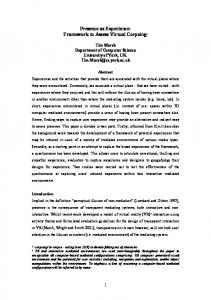
Example 1.1 A bank planner wishes to locate 4 ATMs in the area shown in Figure l ( a ) to serve the customers who are represented by points in the figure. In such a situation, however, natural obstacles exist in the area and they should not be ignored. This is because ignoring these obstacles will result in clusters like those in Figure 1(b) which are obviously inappropriate. For example, Cluster C11 is, as a result of clustering, split by a river, and some customers on one side of the river will have to travel a long way to the ATM located at the other side. 0 Example 1.1 shows a simple but a serious fact which has not been addressed so far: most clustering algorithms assume direct Euclidean distance among the objects to be clustered without obstacles in the way, however, most applications do have obstacles in presence, and the omission of such obstacles may lead to distorted and often useless clustering results. In this study, we examine the problem of clustering spatial objects with the presence of obstacles. The definition of the problem that we are solving is as follows.
Introduction
1
Cluster analysis, which groups data for finding overall distribution patterns and interesting correlations among data sets, has numerous applications in pattern recognition, spatial data analysis, image processing, market research, etc. Cluster analysis has been an active area of research in computational statistics and data mining, with many effective and scalable clustering methods developed recently. These methods can be categorized into partitioning methods [KR90, NH94, BFR981, hierarchical methods [KR90, ZRL96, GRS98, KHK991, density-based methods [EKSX96, ABKS99, HK981, grid-based methods
Definition 1.1 The Clustering with Obstructed Distance (COD ) Problem Given (1) a set P of n points {pl,p2, ...,p n } , and (2) a set 0 of m non-intersecting obstacles (01, ..., om} in a two-dimensional region, R, with each obstacle 0, represented by a simple polygon, the direct Euclidean distance between two points p j and pk, denoted as d(pj,pk), is the Euclidean distance between
~~~~
*The work was supported in part by the Natural Sciences and Engineering Research Council of Canada (NSERC-A3723) and the Networks of Centres of Excellence of Canada (NCE/IRIS-3 and NCE/GEOID)
359 1063-6382/01 $10.00 0 2001 IEEE
the two points by ignoring the obstacles; whereas the obstructed distance, between the two points, denoted ( I S d'(pj, p k ) , is defined as the length of the shortest Euclidean path from pj to pk without cutting through any obstacles. The problem of clustering with obstacle distance (COD) is to partition P into k clusters, C11, . . . . elk, such that the following square-error function, E , is minimized.
where ci is the center of cluster Cli that is determined by the clustering. 0
0
0
0
0 0
0
======
7;
0 .
0 0.
0 0.
/ , J o 0 ~ ~ 0
river
0
0
.
0
0
.
0 . .
.
0
(a) Customers' locations and obstacles.
.*. 00
......
....::,.o..... ....... .;..,
1 ........
'.+ "...
0
: .. 0".
j
'.,
.xc!2.I0 0 0
0 0 0
.i
:.;
......
......._e ............
(b) Clusters formed when ignoring obstacles.
Figure 1. Planning the locations of ATMs Since our given problem is to ensure a minimized overall travel distances of all the customers in the city, the partitioning-based algorithms will be a good choice as a solution. This is because most of the other categories of clustering algorithm focus on finding natural clusters which do not guarantee minimization of the distances to the cluster centers. Of the two typical types of partitioning-based algorithms, k-means and k-medoids, the k-medoids method
0
Zo mean
0
0
0 0
medoid
Figure 2. Mean vs Medoid. is selected due to the fact that the mean of a set of points is not well defined when obstacles are involved. For example, in Figure 2, the mean of the points is inside an obstacle and thus by definition is unreachable by all the points in the cluster. On the other hand, the k-medoids method chooses an object within the cluster as a center and thus ensures that such a problem does not exist. In view of this, we derived an efficient kmedoids algorithm called COD algorithm for solving this problem. The COD-CLARANS algorithm is developed in the spirit of CLARANS [NH94] and is designed for handling obstacles. While CLARANS algorithm can be made to handle obstacles by changing its distance function, COD-CLARANS further optimized this function by "pushing" the task of handling obstacles into the algorithm. Figure 3 shows the overall structure of CODCLARANS. To facilitate the running of CODCLARANS, we pre-process the d a t a and store certain information which will be needed by COD-CLARANS during its run. Pre-processing will 'be discussed in Section 2. The COD-CLARANS algorithm consists of three main parts, the main algorithm] the computation of the squared-error E and a pruning function E'. The pruning function E' has two purposes. First, it can help to prune off search and avoid the computation of E . Second, in the event when the computation of E cannot be avoided, the pruning function can provide focusing information to make the computation of E more efficient. Section 3 will describe them in more detail. In Section 4, we will do a performance study on the COD-CLARANS algorithm. We will discuss some possible future work in Slection 5. Our study is concluded in Section 6.
2
Pre-processing
During the course of clustering,the COD-CLARANS often needs to compute the obstructed distance between a point and a temporary cluster center. Our aim of pre-processing here is t o materialize information which will facilitate such a computation.
360
( Preprocessed Information)
adding two additional nodes p’ and q’ i n V’ representing p and q . Similar t o earlier definition, E’ contains an edge joining two nodes i n V’ if the points represented by the two nodes are mutually visible. T h e shortest path between the two points p and q will be a sub-path of
II Main Function V
Computation of E
VG’.
Figure 3. Overview of COD-CLARANS. .... .. .............. ...... .................... ......................... .. ....... .................. r
0
In Figure 4 , we show how the visibility graph VG’ can be derived from the visibility graph V G of a region with two obstacles 01 and 02. From Lemma 2.1, we can see that the shortest path from p to q will begin with an edge from p to either 211, v2 or 213, go through some path in V G and then end with an edge from either 214 or v5 to q.
I
2.3
Micro-clustering In order for COD-CLARANS to handle a large number of data points, we use the concept of pre-clustering which is similar to those used in BIRCH [ZRL96], ScaleKM [BFR98] and CHAMELEON [KHK99]. A micro-cluster is a compressed representation of a group of points which are so close together that they are likely t o belong to the same cluster. As such, instead of representating each point in the microcluster individually, we represent them using their center and a count of the number of points in the micro-clusters. Using this summarized information, the COD-CLARANS algorithm can approximate the squareerror function E by assuming that all the points in the micro-clusters are located a t the center of the microcluster. To ensure that not too much accuracy is sacrificed by using micro-cluster, we limit the radius of each micro-cluster to be below a user-specified threshold, max-radius. With the presence of obstacles, one key complication is to avoid having a micro-cluster that is split by an obstacle. To do so, we first triangulate the region R into triangles [O’R98] and group the data points according to the triangle that they are in. Figure 5 illustrates a triangulation of the region and the forming of micro-clusters within each triangle. Since all the points within a triangle are always mutually visible, it is guaranteered that no micro-cluster will be split by an obstacle.
VG’
Figure 4. A visibility graph.
2.1
The BSP-tree The Binary-Space-Partition (BSP) tree [SG97] is a data structure which can efficiently determine whether two points p and q are visible to each other within the region R. We define p to be visible from q in the region R if the straight line joining p and q does not intersect any obstacles. In our algorithm, the BSP-tree is used to determine the set of all visible obstacle vertices from a point p. Henceforth, we will use the notation v i s ( p ) to denote such a set of vertices. More details of the BSP-tree can be found in [SG97].
2.2
The Visibility Graph
Definition 2.1 Visibility Graph Given a set of m obstacles, 0 = (01, ..., om}, the visibility graph is a graph V G = (V,E ) such that each vertex of the obstacles has a corresponding node in V , and two nodes v1 and 212 in V are joined by an edge in E if and only i f the corresponding vertices they represent 0 are visible to each other.
To generate V G , we make use of the BSP-tree computed previously and search all other visible vertices from each vertex of the obstacles. The visibility graph is pre-computed because it is useful for finding the obstructed distance between any two points in the region. The following lemma is proven in [O’R98].
2.4 Spatial Join Index While the information described earlier is sufficient for computing the obstructed distance efficiently, improvements can be achieved by the additional computation of a spatial join index [Va187, Rot91, LH921. In such an index, each entry is a 3-tuple ( p ,q , d’(p, q ) ) where p and q are two points in the region R and d’(p, q ) is the obstructed distance between p and q . There are three spatial join indexes which can be materialized:
Lemma 2.1 Let p and q be two points in the region R and V G = (V,E ) be the visibility graph of R. Let VG’ = (VI,E’) be a visibility graph created from V G by 361
3
The COD-CLARANS Algorithm
In this section, we look at the COD-CLARANS algorithm in detail.
3.1 The Main Function
Figure 5. Forming micro-clusters.
1. VV Index: Compute an index entry for any pair of obstacles vertices The materialization of this index is equivalent to finding the all-pairs shortest paths in the visibility graph V G . We make use of the Johnson’s algorithm [CLRSO] for this purpose. From Lemma 2.1, we can see that the computation of shortest path between two points in R will often require the calculation of obstructed distance between the vertices. As such materializing the VV index will help avoid the redundant computation of these distances. 2. MV Index: Compute an index entry for any pair of micro-cluster and obstacles vertex In such an index, the obstructed distance between any pair of micro-cluster and vertex will be computed. An efficient way to materialize the MV index is to first materialize the BSP-tree and the VV index. For each micro-cluster p , the set of visible obstacle vertices, u i s ( p ) can then be computed by using the BSP-tree and the distance to other non-visible be computed by using the VV Index.
We show the main function of the COD-CLARANS algorithm in Algorithm 3.1. The algorithm first randomly selects k points as the centers of the clusters and then tries to find better solutions by iterating through Step 5 to Step 26. At each iteration, the cluster centers are randomly ordered, and attempts will be made to replace them with a better ceni,er in that order. When a center cj is selected to be replaced, the obstructed distances of the objects to the other k - 1 centers in r e m a i n will first be computed in Step 10. This information is computed because they can be repeatedly used in the loop from Step 11 to Step 22 for the computation of E’ and E . In Step 12, a random object C T a n d o m is selected to replace c J . Using C r a n d o m , a lower bound for the squared-error E’ is computed. If E’ is higher than the previous best solution, the actual squared-error E need not be computed since C r a n d o m is obviously a bad choice. Otherwise, E is computed to determine whether a better solution has been found. If this is so, the best solution will be updated and crandom will replace the position of cj in current. For each cluster center, an attempt to replace it will be done m a z - t r y times, if no better solution is found for all the centers, the algorithm terminates.
3.2 Computing Obstructed Distance to Nearest Centers in r e m a i n In this section, the execution of Step 10 is discussed. We separate this step into two phases:
3. MM Index: Compute an index entry for any pair of micro-clusters By computing this index, the obstructed distance between any two micro-clusters will be materialized. Having the MM index means that COD-CLARANS algorithm will performed like the CLARANS algorithm since a lookup on the index is sufficient t o find the obstructed distance between any two micro-clusters. However, the size of such an index will be huge. Thus, we feel that such an alternative will not be feasible.
Algorithm 3.2 Computang Dastances between Objects and Cluster Centres Phase I: For all vertzces of the obstacles, find the shortest obstructed dastance t o the nearest cluster center zn r e m a i n . G w e n a vertex U , we denote zts nearest cluster center as N ( u ) . Phase 11: For each mzcro-clusterp, let us denote the set of all vaszble obstacle vertzces from p as uis(p). W e choose U from u i s ( p ) such that ( d ’ ( u , N ( u ) ) d ( p ,U ) ) 2s manamum. The shortest dzstance between p and ats nearest cluster center wzll be computed as (d’(v,N ( u ) ) + d ( p ,U ) ) and p ’s nearest cluster center an r e m a i n wzll be N ( u ) .
We will compare the relative performance of the first and second alternatives in Section 4.
The execution of Phase I can differ depending on whether the spatial join indexes VV and MV have been materialized. We separate them into three cases.
+
362
c and a vertex v if v is visible from c . In addition, a virtual node s is also inserted and linked by an edge of weight zero t o each of the k - 1 cluster centers. The Dijkstra’s algorithm is then ran with the virtual node s as the source point. To identify the closest cluster center for a vertex w , the shortest path from s to v is traced during the run of Dijkstra’s algorithm to monitor which cluster center is in the path. This cluster center will be the cluster center that is closest to U.
A l g o r i t h m 3.1 Algorithm COD-CLARANS . Input: A set of n objects, k and clustering parameters, m a i t r y . Output: A partition of the n objects into k clusters with cluster centers, c1, ..., ck. Method:
1. Function COD-CLARANSO 2. { randomly select k objects to be current; 3. compute square-error function E; 4. let currentE = E; 5. do 6. { foundnew = FALSE; 7. randomly reorder current into { c l , ..., ck}; 8. for (j=1 ; jsk ; j++) 9. { let remain = current - c3 ; /* remain contain the remaining center */ 10. compute obstructed distance of objects to nearest center in remain; 11. for (try=@ try < maz-try; try++) 12. { replace c3 with a randomly selected object Crandom ; compute estimated square-error function E’; 13. 14. if (E’ > currentE) continue; /* Not a good solution */ 15. 16. compute square-error function E; if ( E < currentE) /* Is the new solution better ? */ 17. { foundnew = TRUE; /* Found a better solution */ 18. current = { c l , ...,crandom,...ck} 19. /* replace c, with Crandom */ 20. currentE = E; 21. 1 22. } 23. if (foundnew) break; /* Reorder cluster centers again */ 24. } 25. 26. } while (foundnew) 28. output current ; 27)
Once Phase I is completed, the execution of Phase I1 is trivial except for forming of vis(p) with respect to a point p . We make use of the BSP-tree for this purpose.
3.3 Computing the Lower Bound E’ After Crandom is generated at line 13 of Algorithm 3.1, we first underestimate the distance between C,andom and the micro-clusters by using direct Euclidean distance. Note that in Step 10, we have already computed the nearest cluster centers from remain for each object p . Let us denote this center as N ( p ) . If the direct Euclidean distance between a micro-cluster p and Crandom is shorter than d’(p, N ( p ) ) (which is also computed with the k - 1 unchanged cluster centers), then p is assigned to Crandom and the direct Euclidean distance between them will be used when computing the estimated square-error function E‘. We have the following lemma.
Lemma 3.1 E‘ is a lower bound f o r the actual squareerror function E . The proof of the Lemma 3.1 is omitted for lack of apace. Since E’ is a lower bound of E , we can choose to abandon Crandom if E’ is already higher than the square-error function of the best solution found so far. However, if E’ is lower than the best solution, then E must be computed. Since the obstructed distance of each micro-cluster p to N ( p ) is already calculated, what we need to find is the obstructed distance between the new center Crandom and the micro-clusters that will be assigned to Crandom. For this purpose, we can use of the focusing information provided by the computation of E’ to limit the set of micro-clusters which will have Crandom as the nearest center. This is done by observing the following lemma.
1. VV is materialized If VV is computed, then all we have to do is to find the visible vertices from each cluster center ci and then compute the obstructed distance of each vertex vj as d’(ci,vj) = m i n ( d ( c i , v k )+ d’( vj , vk)), v k E vis( c i ) . The nearest center of each vertex can then be identified.
2. MV is materialized If MV is available, the obstructed distance between any cluster center and any obstacles vertex will be materialized. As such, a search in MV will be sufficient t o find the obstructed distance of a node v to the IC - 1 centers. The nearest center of the vertex can then be determined.
3. No spatial join index is materialized
Lemma 3.2 I f a micro-cluster p is not assigned to Crandom when computing E’, then it can never be assigned to Crandom when computing E .
If no spatial join index is available, then the precomputed visibility graph V G = (V,E ) will be utilized. We make use of the Dijkstra’s algorithm [CLRSO] for this purpose. We insert k - 1 additional nodes representing the k - 1 cluster centers into V . An edge is created between a cluster center
Using Lemma 3.2, we can limit our computation of obstructed distance t o CTandom to a subset of microclusters instead of all micro-clusters.
363
3.4 Computing the Squared-error E As mentioned earlier, since the obstructed distance of each micro-cluster to its nearest center in remain is already computed in Step 10, what we only need to find when computing E is the obstructed distance between the new center crQndom and the micro-clusters that will be assigned to crandom. This process is similar to Step 10 except that we can use the focusing information provided by E’ to limit the computation.
4
Performance Study
In this section, we will have a look a t the performance of the COD-CLARANS algorithm by performing experiments on a PC with a Pentium 6OOMhz processor and a IBM 7200rpm hard disk. For these experiments, we use two synthetic datasets, DS1 and DS2, which are shown in Figure 6. DS1 consists of 63350 points randomly distributed in the region. We simulate major “obstacles” like rivers, highways] and industrial parks in the region by adding in 20 obstacles. These polygons have a total of 194 edges. DS2 dataset consists of five clusters that are cut through by “stick” obstacles. There are altogether 60000 points and 10 obstacles in DS2. Each obstacle has 4 edges. In our experiments, we set the parameter max-try to be 40. Micro-clusters are formed by applying the BIRCH algorithm described in [ZRL96]. The experiments proceed as follows. First, we as-
(a) DS1.
sess the efficiency and effectiveness of the various fla-
vor of COD-CLARANS by running our algorithms on DS1. COD-CLARANS can be separated into three categories in term of materialized index: 1) non materialized, 2) VV materialized and 3) MV materialized. We denote them as COD-CLARANS-N, COD-CLARANSVV, and COD-CLARANS-MV, respectively. In addition, a symbol “%” will be appended to the end of these algorithms to denote a version in which the pruning function is not used. We assess these algorithms by adjusting the parameter maz-radius that control the number of micro-clusters being formed. Next, we look at the clustering result of COD-CLARANS on DS2 and compare it to those of CLARANS which ignore obstacles in its clustering.
4.1
(b) DS2.
Figure 6. Two datasets. max-radius is increased, we like tal investigate how the quality of the clusters is affected by the use of microclustering. Second, since the number of micro-clusters varies according to max-radius, we can investigate how the various algorithms scale up as the number of microclusters increases. Performing this as a scalability test is preferable over arbitrarily adding points which may affect the distribution of the data and subsequently the execution time of the algorithms. The various values of max-radius and the number of micro-clusters which are formed for DS1 shown in Table 1 together with the average squared-error of the clusters. As can be seen, the increase in the quality of the
Varying max-radius
In this experiment, we vary the number of microclusters that are generated from DS1 by tuning the parameter max-radius that bound the radius of the micro-clusters being formed. There are two purposes in doing this. First, since more accuracy will be lost when
364
,
2wo
Table 1. Effect of Varvina max-radius.
1sw
63350
1Bm
,
,
,
,
I
,
,
C O E C U ~ S - N +-
W E - C W N S W ---*-WECLARANS-MV ...a... COECURANS-NX -e-COECLARANSW% t WE-CLARANSYV% -0 -
*;,
--
is, . *.. .%*.
I
0.02
0.03 0.04
3133 1546
I
I
1.56 1.59
I
965 520
I
0.05
I
1.51 1.55
-
~
12M
1WO 803 Em
400
clusters due to micro-clustering is not significant comparing t o the decrease in the number of micro-clusters for DS1. The drop in cluster quality by performing micro-clustering is at most 8%. Let us now look at the pre-processing time that is required for DS1 in Figure 7. The pre-processing time for COD-CLARANS-N and COD-CLARANS-VV are only minorly affected by max-radius. This is because the only pre-processing operation that max-radius has an effect on is the forming of micro-clusters. We can also see that COD-CLARANS-VV has a higher preprocessing time due to the materialization of the VV index which is equivalent to an all-pair shortest path search on the visibility graph. COD-CLARANS-MV, on the other hand, will decrease with as max-radius increases. This is because increasing max-radius will result in less micro-clusters and corresponding the amount of computation that much be done to calculate the obstructed distance between each micro-clusters and the obstacles vertices. Next, let us look at the actual running time of our algorithm for DS1 in Figure 8. From the graph, we have the following observations. ,
Bm-
sm
E =
300
200
,
,
,
,
,
0 0
,
COEcLAkANsN -+COE-CLARANSW .--X--WECURANS-MV -..*-..
'.,
.......
I
.................*.................*
............
.*-. ................. .................. ..................x*....................==...
.......=...." .
0.01
0.015
0.02
0.025
0.W
0.W5
0.01
0.M
0.S
I
d
onds when max-radius is set to 0.00 and 0.01 respectively. When spatial join indexes are available, the differences between the pruning and non-pruning versions are narrower. This is because the computation of obstructed distance is more efficient with the use of spatial join indexes and thus the reduction of processing time through the pruning function becomes less significant. Second, the spatial join indexes are useful in reducing the execution time of the algorithms. This is true even when the pre-processing times are taken into consideration. For the pruning versions of the CODCLARANS algorithm, having spatial indexes will improve the execution times of the algorithms marginally. Having spatial join indexes in the non-pruning versions of the algorithm however, has significant advantages over one that does not have spatial join indexes. Between the two spatial join indexes, VV and MV, having the MV index generally gives better performance than having the VV index. The only exception is observed for DS1 when the number of micro-clusters is high. In such a case, the size of MV is much higher than the size of VV and the time taken to access MV will offset the advantage that it has by storing more information. As a whole, we found that the COD-CLARANS algorithm scales well for large number of points. We recommend the use of spatial join index MV if the number of edges is small. However, the use of spatial join index VV will be more space efficient since the obstructed distance between any two obstacle vertices is sufficient to avoid running the Dijkstra algorithm on the visibility graph.
-
100:;
0.005
Figure 8. Algorithms Running Time of DS1.
- !'.
400-
-
,
2w
.
Figure 7. Pre-processing Time of DS1.
4.2
First, algorithms which does not use the pruning function will have a longer execution time than those with pruning function. This is especially true for CODCLARANS-N% when the number of micro-clusters is high. The execution time of COD-CLARANS-N% on DS1 reach as high as 66392 seconds and 3119 sec-
Clustering Results
To ascertain that clustering with consideration of obstacles is in fact useful, we will compare the cluster quality of COD-CLARANS with the clusters that is discovered by the CLARANS algorithm. For the 365
CLARANS algorithm, we first cluster the data points by ignoring the obstacles. At the end of the algorithm, the cluster centers are fixed. Data points are then allocated to the nearest centers by obstructed distance and the squared-error will be computed. Note that in this case, points which are earlier assigned to a cluster center may be reassigned to a different one when obstacles are taken into consideration. The results of the two algorithms for DS2 are shown in Figure 9. When k = 5, the average squared-error found by the COD-CLARANS algorithm on DS2 is 1.24 while CLARANS gives an average squared-error of 1.68. The clustering result of DS2 illustrates why CODCLARANS performs better than CLARANS in both cases. Let us refer to the space between any two obstacles as a corridor. As we can see, the cluster centers that are discovered by the COD-CLARANS algorithm are mostly placed at the “entrance” of the corridor so that they are accessible by points from other corridors. On the other hand, CLARANS which has no knowledge of the obstacles will place the centers into the corridors, which means that points from other corridors will be very far from the nearest center. While the performance of COD-CLARANS is better than CLARANS for low value of k , this performance gap is found to decrease as we increase k. The reason behind this is that as k increases, most points will be directly visible to the nearest center. As such, the effect of the obstacles will diminish. We thus conclude that COD-CLARANS will be effective for value of k in which most point will not be directly visible from any of the k centers.
5
(a)Result of COD-CLARANS.
Future Work
While the work presented here is sufficient for many applications of clustering with obstructed distance, there are still a lot of future work to be considered. Although the model of discussion in this paper is in a two-dimensional region with obstacles represented as simple polygons, it can be generalized to other models as well. For example, consider clustering objects around a network structure. We can still perform micro-clustering although there is no requirement for other pre-processing information. To speed up the process, a spatial join index can still be materialized. A pruning function E’ can also be used to prune the search space. In our work, one implicit assumption is that the number of obstacles is smaller than the number of data points. This is true for many applications like ATM locations planning where we only need to take major obstacles into consideration. However, in cases where there are a lot of obstacles between any two data points,
(b) Result of CLARANS.
Figure 9. Clustering Result for DS2. techniques like micro-clustering will not be applicable since a triangulation of the region will result in few or no points in each triangular region. Further study is required to handle such cases. Besides this, a look at how obstacles will affect other clustering paradigms will be interesting as well. For example, it will be challenging to see how density-based algorithms like DBSCAN [EKSX96] can be enhanced to cluster under obstructed distance. Since DBSCAN makes uses of the k-nearest-neighbors operation to perform clustering, an immediate subproblem is to find the k nearest neighbors with consideration of obstacles. This subproblem is a challenge by itself as most
366
k-nearest-neighbors implementation are relying on spatial index structures like the R-tree to speed up the operation and no consideration of obstacles are taken in such a spatial data structure [BBKK97].
6
[EKSX96] M. Ester, H.-P. Kriegel, J. Sander, a n d X. Xu. A density-based algorithm for discovering clusters in large spatial databases. In Proc. 1996 Int. Conf. Knowledge Discovery and Data Mining (KDD’96), pages 226-231, Portland, Oregon, Aug. 1996. [GRS98]
S. Guha, R. Rastogi, a n d K. Shim. Cure: An efficient clustering algorithm for large databases. In Proc. 1998 AGM-SIGMOD Int. Conf. Management of Data (SIGMOD’98), pages 73-84, Seattle, WA, June 1998.
[HK98]
A. Hinneburg and D. A. Keim. An efficient a p proach t o clustering in large multimedia databases with noise. In Proc. 1998 Int. Conf. Knowledge Discovery and Data Mining (Ii‘DD’98), pages 58-65, New York, NY, Aug. 1998.
[KHK99]
G. Karypis, E. - H. Han, and V. Kumar. CHAMELEON: A hierarchical clustering algorithm using dynamic modeling. COMPUTER, 32:68-75, 1999.
[Koh82]
T. Kohonen. Self-organized formation of topologically correct feature maps. Biological Cybernetics, 43:59-69, 1982.
[KR90]
L. Kaufman and P. J. Rousseeuw. Finding Groups i n Data: an Introduction to Cluster Analysis. John Wiley & Sons, 1990.
[LH92]
W. Lu a n d J. Han. Distance-associated join indices for spatial range search. In Proc. 2992 Int. Conf. Data Engineering (ICDE’92), pages 284-292, Phoenix, AZ, Feb. 1992.
[NH94]
R. Ng a n d J. Han. Efficient and effective clustering method for spatial d a t a mining. In Proc. 1994 Int. Conf. Very Large Data Bases ( V L D B ’94), pages 144-155, Santiago, Chile, Sept. 1994.
[O’R98]
J. O’Rourke. Computational Geometry in C (2nd Ed.). Cambridge University Press, 1998.
[Rot911
D. Rotem. Spatial join indices. In Proc. 1992 Int. Conf. Data Engineering (ICDE’gl), pages 500-509, Kobe, J a p a n , Apr. 1991.
[SCZ98]
G . Sheikholeslami, S. Chatterjee, a n d A. Zhang. Wavecluster: A multi-resolution clustering approach for very large spatial databases. In Proc. 1998 Int. Conf. Very Large Data Bases (VLDB’98), pages 428-439, New York, NY, Aug. 1998.
[SD90]
J.W. Shavlik and T.G. Dietterich. Readings in Machine Learning. Morgan Kaufmann, 1990.
[SG97]
Silicon Graphics. Inc. BSP Tree: Frequently asked questions. http://reality.sgi.com/bspfaq/index.shtml, 1997.
[Val871
P. Valduriez. Join indices. AGM Trans. Database Systems, 12:218-246, 1987.
Conclusion
In this paper, we have studied on the problem of Clustering with Obstructed Distance (COD) which we believe is a very has many practical applications. We formalize the definition of this problem and derive an algorithm COD-CLARANS for solving it. We discuss various types of pre-processed information that could enhance the efficiency of COD-CLARANS . By pushing the handling of obstacles into the COD-CLARANS algorithm instead of abstracting it at the distance function level, we are able to provide a pruning function E’ that greatly enhance the efficiency of COD-CLARANS . We perform various experiments on COD-CLARANS to ascertain its usefulness and scalability. Finally, we discuss some potential enhancements to the COD-CLARANS algorithm. We believe that there is still a lot of room for research in the problem of COD and hope that our work could motivate more people to look into this area.
Acknowledgment: The first author wishes to thank Binay Bhattacharya for introducing the field of Computation Geometry to him. Discussions with Raymond T. Ng and Laks V. S. Lakshmanan have been very useful towards this work. The code for BIRCH is kindly provided by Raghu Ramakrishnan.
References [ABKS99] M. Ankerst, M. Breunig, H.-P. Kriegel, a n d J. Sander. OPTICS: Ordering points t o identify the clustering structure. In Proc. 1999 ACMSIGMOD Int. Conf. Management of Data (SIGMOD’99), pages 49-60, Philadelphia, PA, June 1999. [AGGR98] R.Agrawal, J. Gehrke, D. Gunopulos, a n d P. Raghavan. Automatic subspace clustering of high dimensional d a t a for d a t a mining applications. In Proc. 1998 AGM-SIGMOD Int. Conf. Management of Data (SIGMOD’98), pages 94-105, Seattle, WA, June 1998. [BBKK97] S. Berchtold, C. Bohm, D. A. Keim, and H. P. Kriegel. A cost model for nearest neighbor search in high dimensional d a t a space. In Proc. of 16th A CM Symp. on Principles of Database Systems (PODS), 1997. [BFRSS] P. Bradley, U. Fayyad, and C. Reina. Scaling clustering algorithms t o large databases. In Proc. 1998 Int. Conf. Knowledge Discovery and Data Mining (KDD’98), pages 9-15, New York, NY, Aug. 1998. [CLRSO] T. Cormen, C. Leiserson, and R. Rivest. Introduction to Algorithms. T h e MIT Press, Cambridge, MA, 1990.
[WYM97] W . Wang, J. Yang, and R. Muntz. STING: A statistical information grid approach t o spatial d a t a mining. In Proc. 1997 Int. Conf. Very Large Data Bases (VLDB’97), pages 186-195, Athens, Greece, Aug. 1997. [ZRL96]
T. Zhang, R. Ramakrishnan, and M. Livny. BIRCH: a n efficient d a t a clustering method for very large databases. In Proc. 1996 AGM-SIGMOD Int. Conf, Management of Data (SIGMOD’96), pages 103-114, Montreal, Canada, J u n e 1996.
367