Spatial Domain Methods for Orientation and Velocity Estimation - DiVA

Link¨oping Studies in Science and Technology Thesis No. 755

Spatial Domain Methods for Orientation and Velocity Estimation Gunnar Farneb¨ack

LIU-TEK-LIC-1999:13 Department of Electrical Engineering Link¨opings universitet, SE-581 83 Link¨oping, Sweden Link¨oping March 1999

Spatial Domain Methods for Orientation and Velocity Estimation c 1999 Gunnar Farneb¨ack ° Department of Electrical Engineering Link¨ opings universitet SE-581 83 Link¨ oping Sweden

ISBN 91-7219-441-3

ISSN 0280-7971

iii

To Lisa

iv

v

Abstract In this thesis, novel methods for estimation of orientation and velocity are presented. The methods are designed exclusively in the spatial domain. Two important concepts in the use of the spatial domain for signal processing is projections into subspaces, e.g. the subspace of second degree polynomials, and representations by frames, e.g. wavelets. It is shown how these concepts can be unified in a least squares framework for representation of finite dimensional vectors by bases, frames, subspace bases, and subspace frames. This framework is used to give a new derivation of Normalized Convolution, a method for signal analysis that takes uncertainty in signal values into account and also allows for spatial localization of the analysis functions. With the help of Normalized Convolution, a novel method for orientation estimation is developed. The method is based on projection onto second degree polynomials and the estimates are represented by orientation tensors. A new concept for orientation representation, orientation functionals, is introduced and it is shown that orientation tensors can be considered a special case of this representation. A very efficient implementation of the estimation method is presented and by evaluation on a test sequence it is demonstrated that the method performs excellently. Considering an image sequence as a spatiotemporal volume, velocity can be estimated from the orientations present in the volume. Two novel methods for velocity estimation are presented, with the common idea to combine the orientation tensors over some region for estimation of the velocity field according to a motion model, e.g. affine motion. The first method involves a simultaneous segmentation and velocity estimation algorithm to obtain appropriate regions. The second method is designed for computational efficiency and uses local neighborhoods instead of trying to obtain regions with coherent motion. By evaluation on the Yosemite sequence, it is shown that both methods give substantially more accurate results than previously published methods.

vi

vii

Acknowledgements This thesis could never have been written without the contributions from a large number of people. In particular I want to thank the following persons: Lisa, for love and patience. All the people at the Computer Vision Laboratory, for providing a stimulating research environment and good friendship. Professor G¨osta Granlund, the head of the research group and my supervisor, for showing confidence in my work and letting me pursue my research ideas. Dr. Klas Nordberg, for taking an active interest in my research from the first day and contributing with countless ideas and discussions. Associate Professor Hans Knutsson, for a never ending stream of ideas, some of which I have even been able to understand and make use of. Bj¨orn Johansson and visiting Professor Todd Reed, for constructive criticism on the manuscript and many helpful suggestions. Drs. Peter Hackman, Arne Enqvist, and Thomas Karlsson at the Department of Mathematics, for skillful teaching of undergraduate mathematics and for consultations on some of the mathematical details in the thesis. Professor Lars Eld´en, also at the Department of Mathematics, for help with the numerical aspects of the thesis. Dr. J¨orgen Karlholm, for much inspiration and a great knowledge of the relevant literature. Johan Wiklund, for keeping the computers happy. The Knut and Alice Wallenberg foundation, for funding the research within the WITAS project.

viii

Contents 1 Introduction 1.1 Motivation . 1.2 Organization 1.3 Contributions 1.4 Notation . . .

. . . .

. . . .

. . . .

. . . .

. . . .

. . . .

. . . .

. . . .

. . . .

. . . .

. . . .

. . . .

. . . .

. . . .

. . . .

. . . .

. . . .

. . . .

. . . .

. . . .

. . . .

. . . .

. . . .

. . . .

. . . .

. . . .

. . . .

. . . .

2 A Unified Framework for Bases, Frames, Subspace Bases, Subspace Frames 2.1 Introduction . . . . . . . . . . . . . . . . . . . . . . . . . . . . . 2.2 Preliminaries . . . . . . . . . . . . . . . . . . . . . . . . . . . . 2.2.1 Notation . . . . . . . . . . . . . . . . . . . . . . . . . . . 2.2.2 The Linear Equation System . . . . . . . . . . . . . . . 2.2.3 The Linear Least Squares Problem . . . . . . . . . . . . 2.2.4 The Minimum Norm Problem . . . . . . . . . . . . . . . 2.2.5 The Singular Value Decomposition . . . . . . . . . . . . 2.2.6 The Pseudo-Inverse . . . . . . . . . . . . . . . . . . . . 2.2.7 The General Linear Least Squares Problem . . . . . . . 2.2.8 Numerical Aspects . . . . . . . . . . . . . . . . . . . . . 2.3 Representation by Sets of Vectors . . . . . . . . . . . . . . . . . 2.3.1 Notation . . . . . . . . . . . . . . . . . . . . . . . . . . . 2.3.2 Definitions . . . . . . . . . . . . . . . . . . . . . . . . . 2.3.3 Dual Vector Sets . . . . . . . . . . . . . . . . . . . . . . 2.3.4 Representation by a Basis . . . . . . . . . . . . . . . . . 2.3.5 Representation by a Frame . . . . . . . . . . . . . . . . 2.3.6 Representation by a Subspace Basis . . . . . . . . . . . 2.3.7 Representation by a Subspace Frame . . . . . . . . . . . 2.3.8 The Double Dual . . . . . . . . . . . . . . . . . . . . . . 2.3.9 A Note on Notation . . . . . . . . . . . . . . . . . . . . 2.4 Weighted Norms . . . . . . . . . . . . . . . . . . . . . . . . . . 2.4.1 Notation . . . . . . . . . . . . . . . . . . . . . . . . . . . 2.4.2 The Weighted General Linear Least Squares Problem . 2.4.3 Representation by Vector Sets . . . . . . . . . . . . . . 2.4.4 Dual Vector Sets . . . . . . . . . . . . . . . . . . . . . . 2.5 Weighted Seminorms . . . . . . . . . . . . . . . . . . . . . . . .

. . . .

. . . .

1 1 2 2 3

and . . . . . . . . . . . . . . . . . . . . . . . . . .

. . . . . . . . . . . . . . . . . . . . . . . . . .

5 5 5 5 6 6 6 7 7 8 8 8 8 9 9 9 10 10 10 11 11 12 12 12 12 13 14

x

Contents 2.5.1 2.5.2

The Seminorm Weighted General Linear Least Squares Problem . . . . . . . . . . . . . . . . . . . . . . . . . . . . . . . Representation by Vector Sets and Dual Vector Sets . . . .

3 Normalized Convolution 3.1 Introduction . . . . . . . . . . . . . . . . . . . . . . 3.2 Definition of Normalized Convolution . . . . . . . . 3.2.1 Signal and Certainty . . . . . . . . . . . . . 3.2.2 Basis Functions and Applicability . . . . . . 3.2.3 Definition . . . . . . . . . . . . . . . . . . . 3.2.4 Comments on the Definition . . . . . . . . . 3.3 Implementational Issues . . . . . . . . . . . . . . . 3.4 Example . . . . . . . . . . . . . . . . . . . . . . . . 3.5 Output Certainty . . . . . . . . . . . . . . . . . . . 3.6 Normalized Differential Convolution . . . . . . . . 3.7 Reduction to Ordinary Convolution . . . . . . . . . 3.8 Application Examples . . . . . . . . . . . . . . . . 3.8.1 Normalized Averaging . . . . . . . . . . . . 3.8.2 The Cubic Facet Model . . . . . . . . . . . 3.9 Choosing the Applicability . . . . . . . . . . . . . . 3.10 Further Generalizations of Normalized Convolution

14 15

. . . . . . . . . . . . . . . .

. . . . . . . . . . . . . . . .

. . . . . . . . . . . . . . . .

. . . . . . . . . . . . . . . .

. . . . . . . . . . . . . . . .

. . . . . . . . . . . . . . . .

. . . . . . . . . . . . . . . .

17 17 18 18 19 19 20 21 22 23 24 25 27 27 30 31 31

4 Orientation Estimation 4.1 Introduction . . . . . . . . . . . . . . . . . . . . . . . . . 4.2 The Orientation Tensor . . . . . . . . . . . . . . . . . . 4.2.1 Representation of Orientation for Simple Signals 4.2.2 Estimation . . . . . . . . . . . . . . . . . . . . . 4.2.3 Interpretation for Non-Simple Signals . . . . . . 4.3 Orientation Functionals . . . . . . . . . . . . . . . . . . 4.4 Signal Model . . . . . . . . . . . . . . . . . . . . . . . . 4.5 Construction of the Orientation Tensor . . . . . . . . . . 4.5.1 Linear Neighborhoods . . . . . . . . . . . . . . . 4.5.2 Quadratic Neighborhoods . . . . . . . . . . . . . 4.5.3 General Neighborhoods . . . . . . . . . . . . . . 4.6 Properties of the Estimated Tensor . . . . . . . . . . . . 4.7 Fast Implementation . . . . . . . . . . . . . . . . . . . . 4.7.1 Equivalent Correlation Kernels . . . . . . . . . . 4.7.2 Cartesian Separability . . . . . . . . . . . . . . . 4.8 Computational Complexity . . . . . . . . . . . . . . . . 4.9 Relation to First and Second Derivatives . . . . . . . . . 4.10 Evaluation . . . . . . . . . . . . . . . . . . . . . . . . . . 4.10.1 The Importance of Isotropy . . . . . . . . . . . . 4.10.2 Gaussian Applicabilities . . . . . . . . . . . . . . 4.10.3 Choosing γ . . . . . . . . . . . . . . . . . . . . . 4.10.4 Best Results . . . . . . . . . . . . . . . . . . . . 4.11 Possible Improvements . . . . . . . . . . . . . . . . . . .

. . . . . . . . . . . . . . . . . . . . . . .

. . . . . . . . . . . . . . . . . . . . . . .

. . . . . . . . . . . . . . . . . . . . . . .

. . . . . . . . . . . . . . . . . . . . . . .

. . . . . . . . . . . . . . . . . . . . . . .

. . . . . . . . . . . . . . . . . . . . . . .

33 33 34 34 35 35 35 37 38 39 39 41 42 44 45 45 50 53 54 56 59 59 59 61

. . . . . . . . . . . . . . . .

. . . . . . . . . . . . . . . .

Contents

xi

4.11.1 Multiple Scales . . . . . . . . . . . . . . . . . . . . . . . . . 4.11.2 Different Radial Functions . . . . . . . . . . . . . . . . . . . 4.11.3 Additional Basis Functions . . . . . . . . . . . . . . . . . . 5 Velocity Estimation 5.1 Introduction . . . . . . . . . . . . . . . . . . . . . . . 5.2 From Orientation to Motion . . . . . . . . . . . . . . 5.3 Estimating a Parameterized Velocity Field . . . . . . 5.3.1 Motion Models . . . . . . . . . . . . . . . . . 5.3.2 Cost Functions . . . . . . . . . . . . . . . . . 5.3.3 Parameter Estimation . . . . . . . . . . . . . 5.4 Simultaneous Segmentation and Velocity Estimation 5.4.1 The Competitive Algorithm . . . . . . . . . . 5.4.2 Candidate Regions . . . . . . . . . . . . . . . 5.4.3 Segmentation Algorithm . . . . . . . . . . . . 5.5 A Fast Velocity Estimation Algorithm . . . . . . . . 5.6 Evaluation . . . . . . . . . . . . . . . . . . . . . . . . 5.6.1 Implementation and Performance . . . . . . . 5.6.2 Results for the Yosemite Sequence . . . . . . 5.6.3 Results for the Diverging Tree Sequence . . .

61 62 62

. . . . . . . . . . . . . . .

63 63 63 64 65 65 67 69 70 70 71 72 75 76 77 82

6 Future Research Directions 6.1 Phase Functionals . . . . . . . . . . . . . . . . . . . . . . . . . . . 6.2 Adaptive Filtering . . . . . . . . . . . . . . . . . . . . . . . . . . . 6.3 Irregular Sampling . . . . . . . . . . . . . . . . . . . . . . . . . . .

85 85 86 88

. . . . . . . . . . . . . . .

. . . . . . . . . . . . . . .

. . . . . . . . . . . . . . .

. . . . . . . . . . . . . . .

Appendices A A Matrix Inversion Lemma . . . . . . . . . . . . . . . . . . B Cartesian Separable and Isotropic Functions . . . . . . . . . C Correlator Structure for Separable Normalized Convolution D Angular RMS Error . . . . . . . . . . . . . . . . . . . . . . E Removing the Isotropic Part of a 3D Tensor . . . . . . . . .

. . . . . . . . . . . . . . .

. . . . .

. . . . . . . . . . . . . . .

. . . . .

. . . . . . . . . . . . . . .

. . . . .

93 . 93 . 95 . 98 . 99 . 100

xii

Contents

Chapter 1

Introduction 1.1

Motivation

In this licenciate thesis, spatial domain methods for orientation and velocity estimation are developed, together with a solid framework for design of signal processing algorithms in the spatial domain. It is more conventional for such methods to be designed, at least partially, in the Fourier domain. To understand why we wish to avoid the use of the Fourier domain altogether, it is necessary to have some background information. The theory and methods presented in this thesis are results of the research within the WITAS1 project [57]. The goal of this project is to develop an autonomous flying vehicle and naturally the vision subsystem is an important component. Unfortunately the needed image processing has a tendency to be computationally very demanding and therefore it is of interest to find ways to reduce the amount of processing. One way to do this is to emulate biological vision by using foveally sampled images, i.e. having a higher sampling density in an area of interest and gradually lower sampling density further away. In contrast to the usual rectangular grids, this approach leads to highly irregular sampling patterns. Except for some very specific sampling patterns, e.g. the logarithmic polar [10, 42, 47, 58], the theory for irregularly sampled multidimensional signals is far less developed than the corresponding theory for regularly sampled signals. Some work has been done on the problem of reconstructing irregularly sampled bandlimited signals [16]. In contrast to the regular case this turns out to be quite complicated, one reason being that the Nyquist frequency varies spatially with the local sampling density. In fact the use of the Fourier domain in general, e.g. for filter design, becomes much more complicated and for this reason we turn our attention to the spatial domain. So far all work has been restricted to regularly sampled signals, with adaptation of the methods to the irregularly sampled case as a major future research goal. Even without going to the irregularly sampled case, however, the spatial domain 1 Wallenberg

laboratory for Information Technology for Autonomous Systems.

2

Introduction

approach has turned out to be successful, since the resulting methods are efficient and have excellent accuracy.

1.2

Organization

An important concept in the use of the spatial domain for signal processing is projections into subspaces, e.g. the subspace of second degree polynomials. Chapter 2 presents a unified framework for representations of finite dimensional vectors by bases, frames, subspace bases, and subspace frames. The basic idea is that all these representations by sets of vectors can be regarded as solutions to various least squares problems. Generalizations to weighted least squares problems are explored and dual vector sets are derived for efficient computation of the representations. In chapter 3 the theory developed in the previous chapter is used to derive the method called Normalized Convolution. This method is a powerful tool for signal analysis in the spatial domain, being able to take uncertainties in the signal values into account and allowing spatial localization of the analysis functions. Chapter 4 introduces orientation functionals for representation of orientation and it is shown that orientation tensors can be regarded as a special case of this concept. With the use of Normalized Convolution, a spatial domain method for estimation of orientation tensors, based on projection onto second degree polynomials, is developed. It is shown that, properly designed, this method can be implemented very efficiently and by evaluation on a test volume that it in practice performs excellently. In chapter 5 the orientation tensors from the previous chapter are utilized for velocity estimation. With the idea to estimate velocity over whole regions according to some motion model, two different algorithms are developed. The first one is a simultaneous segmentation and velocity estimation algorithm, while the second one gains in computational efficiency by disregarding the need for a proper segmentation into regions with coherent motion. By evaluation on the Yosemite sequence it is shown that both algorithms are substantially more accurate than previously published methods for velocity estimation. The thesis concludes with chapter 6 and a look at future research directions. It is sketched how orientation functionals can be extended to phase functionals, how the projection onto second degree polynomials can be employed for adaptive filtering, and how Normalized Convolution can be adapted to irregularly sampled signals. Since Normalized Convolution is the key tool for the orientation and velocity estimation algorithms, these will require only small amounts of additional work to be adapted to irregularly sampled signals. This chapter also explains how the cover image relates to the thesis.

1.3

Contributions

It is never easy to say for sure what ideas and methods are new and which have been published somewhere previously. The following is an attempt at listing the parts of the material that are original and more or less likely to be truly novel.

1.4 Notation

3

The main contribution in chapter 2 is the unification of the seemingly disparate concepts of frames and subspace bases in a least squares framework, together with bases and subspace frames. Other original ideas is the simultaneous weighting in both the signal and coefficient spaces for subspace frames, the full generalization of dual vector sets to the weighted norm case in section 2.4.4, and most of the results in section 2.5 on the weighted seminorm case. The concept of weighted linear combinations in section 2.4.4 may also be novel. The method of Normalized Convolution in Chapter 3 is certainly not original work. The primary contribution here is the presentation of the method. By taking advantage of the framework from chapter 2 to derive the method, the goal is to achieve greater clarity than in earlier presentations. There are also some new contributions to the theory, such as parts of the discussion about output certainty in section 3.5, most of section 3.9, and all of section 3.10. In chapter 4 everything is original except section 4.2 about the tensor representation of orientation and estimation of tensors by means of quadrature filter responses. The main contributions are the concept of orientation functionals in section 4.3, the method to estimate orientation tensors from the projection onto second degree polynomials in section 4.5, the efficient implementation of the estimation method in section 4.7, and the observation of the importance of isotropy in section 4.10.1. The results on separable computation of Normalized Convolution in sections 5.5 and 4.8 are not limited to a polynomial basis but applies to any set of Cartesian separable basis functions and applicabilities. This makes it possible to do the computations significantly more efficient and is obviously an important contribution to the theory of Normalized Convolution. Chapter 5 mostly contains original work too, with the exception of sections 5.2 and 5.3.1. The main contributions here are the methods for estimation of motion model parameters in section 5.3, the algorithm for simultaneous segmentation and velocity estimation in section 5.4, and the fast velocity estimation algorithm in section 5.5. Large parts of the material in chapter 5 were developed for my master’s thesis and has been published in [13, 14]. The material in chapter 2 has been accepted for publication at the SCIA’99 conference [15].

1.4

Notation

Lowercase letters in boldface (v) are used for vectors and in matrix algebra contexts they are always column vectors. Uppercase letters in boldface (A) are used for matrices. The conjugate transpose of a matrix or a vector is denoted A∗ . The transpose of a real matrix or vector is also denoted AT . Complex conjugation without transpose is denoted v ¯. The standard inner product between two vectors is written (u, v) or u∗ v. The norm of a vector is induced from the inner product, √ (1.1) kvk = v∗ v. Weighted inner products are given by (u, v)W = (Wu, Wv) = u∗ W∗ Wv

(1.2)

4 and the induced weighted norms by p p kvkW = (v, v)W = (Wv, Wv) = kWvk,

Introduction

(1.3)

where W normally is a positive definite Hermitian matrix. In the case that it is only positive semidefinite we instead have a weighted seminorm. The norm of a matrix is assumed to be the Frobenius norm, kAk2 = tr (A∗ A), where the trace of a quadratic matrix, tr M, is the sum of the diagonal elements. The pseudoinverse of a matrix is denoted A† . Somewhat nonstandard is the use of u · v to denote pointwise multiplication of the elements of two vectors. Finally v ˆ is used to denote vectors of unit length and v ˜ is used for dual vectors. Additional notation is introduced where needed, e.g. f ? g to denote unnormalized cross correlation in section 3.7.

Chapter 2

A Unified Framework for Bases, Frames, Subspace Bases, and Subspace Frames 2.1

Introduction

Frames and subspace bases, and of course bases, are well known concepts, which have been covered in several publications. Usually, however, they are treated as disparate entities. The idea behind this presentation of the material is to give a unified framework for bases, frames, and subspace bases, as well as the somewhat less known subspace frames. The basic idea is that the coefficients in the representation of a vector in terms of a frame, etc., can be described as solutions to various least squares problems. Using this to define what coefficients should be used, expressions for dual vector sets are derived. These results are then generalized to the case of weighted norms and finally also to the case of weighted seminorms. The presentation is restricted to finite dimensional vector spaces and relies heavily on matrix representations.

2.2

Preliminaries

To begin with, we review some basic concepts from (Numerical) Linear Algebra. All of these results are well known and can be found in any modern textbook on Numerical Linear Algebra, e.g. [19].

2.2.1

Notation

Let C n be an n-dimensional complex vector space. Elements of this space are denoted by lower-case bold letters, e.g. v, indicating n × 1 column vectors. Uppercase bold letters, e.g. F, denote complex matrices. With C n is associated the

6

A Unified Framework . . .

standard inner product, (f ,p g) = f ∗ g, where ∗ denotes conjugate transpose, and the Euclidian norm, kf k = (f , f ). In this section A is an n × m complex matrix, b ∈ C n , and x ∈ C m .

2.2.2

The Linear Equation System

The linear equation system Ax = b

(2.1)

x = A−1 b

(2.2)

has a unique solution

if and only if A is square and non-singular. If the equation system is overdetermined it does in general not have a solution and if it is underdetermined there are normally an infinite set of solutions. In these cases the equation system can be solved in a least squares and/or minimum norm sense, as discussed below.

2.2.3

The Linear Least Squares Problem

Assume that n ≥ m and that A is of rank m (full column rank). Then the equation Ax = b is not guaranteed to have a solution and the best we can do is to minimize the residual error. The linear least squares problem arg minn kAx − bk

(2.3)

x = (A∗ A)−1 A∗ b.

(2.4)

x∈C

has the unique solution

If A is rank deficient the solution is not unique, a case which we return to in section 2.2.7.

2.2.4

The Minimum Norm Problem

Assume that n ≤ m and that A is of rank n (full row rank). Then the equation Ax = b may have more than one solution and to choose between them we take the one with minimum norm. The minimum norm problem arg min kxk, x∈S

S = {x ∈ C m ; Ax = b}.

(2.5)

has the unique solution x = A∗ (AA∗ )−1 b.

(2.6)

If A is rank deficient it is possible that there is no solution at all, a case to which we return in section 2.2.7.

2.2 Preliminaries

2.2.5

7

The Singular Value Decomposition

An arbitrary matrix A of rank r can be factored by the Singular Value Decomposition, SVD, as A = UΣV∗ ,

(2.7)

where U and V are unitary matrices, n×n and m×m respectively. Σ is a diagonal n × m matrix ¡ ¢ Σ = diag σ1 , . . . , σr , 0, . . . , 0 , (2.8) where σ1 , . . . , σr are the non-zero singular values. The singular values are all real and σ1 ≥ . . . ≥ σr > 0. If A is of full rank we have r = min(n, m) and all singular values are non-zero.

2.2.6

The Pseudo-Inverse

The pseudo-inverse1 A† of any matrix A can be defined via the SVD given by (2.7) and (2.8) as A† = VΣ† U∗ ,

(2.9)

where Σ† is a diagonal m × n matrix ¡ ¢ Σ† = diag σ11 , . . . , σ1r , 0, . . . , 0 .

(2.10)

We can notice that if A is of full rank and n ≥ m, then the pseudo-inverse can also be computed as A† = (A∗ A)−1 A∗

(2.11)

A† = A∗ (AA∗ )−1 .

(2.12)

and if instead n ≤ m then If m = n then A is quadratic and the condition of full rank becomes equivalent with non-singularity. It is obvious that both the equations (2.11) and (2.12) reduce to A† = A−1

(2.13)

in this case. Regardless of rank conditions we have the following useful identities: (A† )† = A ∗ †

(2.14) † ∗

(A ) = (A ) †

∗

(2.15) †

∗

(2.16)

∗ †

(2.17)

A = (A A) A †

∗

A = A (AA ) 1 This

pseudo-inverse is also known as the Moore-Penrose inverse.

8

A Unified Framework . . .

2.2.7

The General Linear Least Squares Problem

The remaining case is when A is rank deficient. Then the equation Ax = b is not guaranteed to have a solution and there may be more than one x minimizing the residual error. This problem can be solved as a simultaneous least squares and minimum norm problem. The general (or rank deficient) linear least squares problem is stated as arg min kxk, x∈S

S = {x ∈ C m ; kAx − bk is minimum},

(2.18)

i.e. among the least squares solutions, choose the one with minimum norm. Clearly this formulation contains both the ordinary linear least squares problem and the minimum norm problem as special cases. The unique solution is given in terms of the pseudo-inverse as x = A† b

(2.19)

Notice that by equations (2.11) – (2.13) this solution is consistent with (2.2), (2.4), and (2.6).

2.2.8

Numerical Aspects

Although the above results are most commonly found in books on Numerical Linear Algebra, only their algebraic properties are being discussed here. It should, however, be mentioned that e.g. equations (2.9) and (2.11) have numerical properties that differ significantly. The interested reader is referred to [5].

2.3

Representation by Sets of Vectors

If we have a set of vectors {fk } ⊂ C n and wish to represent2 an arbitrary vector v as a linear combination X v∼ c k fk (2.20) of the given set, how should the coefficients {ck } be chosen? In general this question can be answered in terms of linear least squares problems.

2.3.1

Notation

n With the set of vectors, {fk }m k=1 ⊂ C , is associated an n × m matrix

F = [f1 , f2 , . . . , fm ],

(2.21)

which effectively is a reconstructing operator because multiplication with an m × 1 vector c, Fc, produces linear combinations of the vectors {fk }. In terms of the reconstruction matrix, equation (2.20) can be rewritten as v ∼ Fc, 2 Ideally

(2.22)

we would like to have equality in equation (2.20) but that cannot always be obtained.

2.3 Representation by Sets of Vectors

linearly

independent dependent

9

spans C n yes no basis subspace basis frame subspace frame

Table 2.1: Definitions where the coefficients {ck } have been collected in the vector c. The conjugate transpose of the reconstruction matrix, F∗ , gives an analyzing operator because F∗ x yields a vector containing the inner products between {fk } and the vector x ∈ C n .

2.3.2

Definitions

Let {fk } be a subset of C n . If {fk } spans C n and is linearly independent it is called a basis. If it spans C n but is linearly dependent it is called a frame. If it is linearly independent but does not span C n it is called a subspace basis. Finally, if it neither spans C n , nor is linearly independent, it is called a subspace frame.3 This relationship is depicted in table 2.1. If the properties of {fk } are unknown or arbitrary we simply use set of vectors or vector set as a collective term.

2.3.3

Dual Vector Sets

We associate with a given vector set {fk } the dual vector set {˜ fk }, characterized by the condition that for an arbitrary vector v the coefficients {ck } in equation (2.20) are given as inner products between the dual vectors and v, ck = (˜ fk , v) = ˜ fk∗ v.

(2.23)

˜ correThis equation can be rewritten in terms of the reconstruction matrix F sponding to {˜ fk } as ˜ ∗ v. c=F

(2.24)

The existence of the dual vector set is a nontrivial fact, which will be proved in the following sections for the various classes of vector sets.

2.3.4

Representation by a Basis

Let {fk } be a basis. An arbitrary vector v can be written as a linear combination of the basis vectors, v = Fc, for a unique coefficient vector c.4 Because F is invertible in the case of a basis, we immediately get c = F−1 v 3 The

(2.25)

notation used here is somewhat nonstandard. See section 2.3.9 for a discussion. coefficients {ck } are of course also known as the coordinates for v with respect to the basis {fk }. 4 The

10

A Unified Framework . . .

˜ exists and is given by and it is clear from comparison with equation (2.24) that F ˜ = (F−1 )∗ . F

(2.26)

In this very ideal case where the vector set is a basis, there is no need to state ˜ That this could indeed be done is discussed a least squares problem to find c or F. in section 2.3.7.

2.3.5

Representation by a Frame

Let {fk } be a frame. Because the frame spans C n , an arbitrary vector v can still be written as a linear combination of the frame vectors, v = Fc. This time, however, there are infinitely many coefficient vectors c satisfying the relation. To get a uniquely determined solution we add the requirement that c be of minimum norm. This is nothing but the minimum norm problem of section 2.2.4 and equation (2.6) gives the solution c = F∗ (FF∗ )−1 v.

(2.27)

Hence the dual frame exists and is given by ˜ = (FF∗ )−1 F. F

2.3.6

(2.28)

Representation by a Subspace Basis

Let {fk } be a subspace basis. In general, an arbitrary vector v cannot be written as a linear combination of the subspace basis vectors, v = Fc. Equality only holds for vectors v in the subspace spanned by {fk }. Thus we have to settle for the c giving the closest vector v0 = Fc in the subspace. Since the subspace basis vectors are linearly independent we have the linear least squares problem of section 2.2.3 with the solution given by equation (2.4) as c = (F∗ F)−1 F∗ v.

(2.29)

Hence the dual subspace basis exists and is given by ˜ = F(F∗ F)−1 . F

(2.30)

Geometrically v0 is the orthogonal projection of v onto the subspace.

2.3.7

Representation by a Subspace Frame

Let {fk } be a subspace frame. In general, an arbitrary vector v cannot be written as a linear combination of the subspace frame vectors, v = Fc. Equality only holds for vectors v in the subspace spanned by {fk }. Thus we have to settle for the c giving the closest vector v0 = Fc in the subspace. Since the subspace frame vectors are linearly dependent there are also infinitely many c giving the same closest vector v0 , so to distinguish between these we choose the one with minimum

2.3 Representation by Sets of Vectors

11

norm. This is the general linear least squares problem of section 2.2.7 with the solution given by equation (2.19) as c = F† v.

(2.31)

Hence the dual subspace frame exists and is given by ˜ = (F† )∗ . F

(2.32)

The subspace frame case is the most general case since all the other ones can be considered as special cases. The only thing that happens to the general linear least squares problem formulated here is that sometimes there is an exact solution v = Fc, rendering the minimum residual error requirement superfluous, and sometimes there is a unique solution c, rendering the minimum norm requirement superfluous. Consequently the solution given by equation (2.32) subsumes all the other ones, which is in agreement with equations (2.11) – (2.13).

2.3.8

The Double Dual

The dual of {˜ fk } can be computed from equation (2.32), applied twice, together with (2.14) and (2.15). ˜ ˜=F ˜ †∗ = F†∗†∗ = F†∗∗† = F†† = F. F

(2.33)

What this means is that if we know the inner products between v and {fk } we can reconstruct v using the dual vectors. To summarize we have the two relations ˜ ∗ v) = v ∼ F(F ˜ ∗ v) = v ∼ F(F

2.3.9

X

(˜ fk , v)fk

and

(2.34)

k

X

(fk , v)˜ fk .

(2.35)

k

A Note on Notation

Usually a frame is defined by the frame condition, X |(fk , v)|2 ≤ Bkvk2 , Akvk2 ≤

(2.36)

k

which must hold for some A > 0, some B < ∞, and all v ∈ C n . In the finite dimensional setting used here the first inequality holds if and only if {f k } spans all of C n and the second inequality is a triviality as soon as the number of frame vectors is finite. The difference between this definition and the one used in section 2.3.2 is that the bases are included in the set of frames. As we have seen that equation (2.28) is consistent with equation (2.26), the same convention could have been used here. The reason for not doing so is that the presentation would have become more involved.

12

A Unified Framework . . .

Likewise, we may allow the subspace bases to span the whole C n , making bases a special case. Indeed, as has already been discussed to some extent, if subspace frames are allowed to be linearly independent, and/or span the whole C n , all the other cases can be considered special cases of subspace frames.

2.4

Weighted Norms

An interesting generalization of the theory developed so far is to exchange the Euclidian norms used in all minimizations for weighted norms.

2.4.1

Notation

Let the weighting matrix W be an n × n positive definite Hermitian matrix. The weighted inner product (·, ·)W on C n is defined by (f , g)W = (Wf , Wg) = f ∗ W∗ Wg = f ∗ W2 g

and the induced weighted norm k · kW is given by p p kf kW = (f , f )W = (Wf , Wf ) = kWf k. n

In this section M and L denote weighting matrices for C and C The notation from previous sections carry over unchanged.

2.4.2

(2.37)

(2.38) m

respectively.

The Weighted General Linear Least Squares Problem

The weighted version of the general linear least squares problem is stated as arg min kxkL , x∈S

S = {x ∈ C m ; kAx − bkM is minimum}.

(2.39)

This problem can be reduced to its unweighted counterpart by introducing x 0 = Lx, whereby equation (2.39) can be rewritten as arg min kx0 k, 0 x ∈S

S = {x0 ∈ C m ; kMAL−1 x0 − Mbk is minimum}.

(2.40)

The solution is given by equation (2.19) as x0 = (MAL−1 )† Mb,

(2.41)

which after back-substitution yields x = L−1 (MAL−1 )† Mb.

2.4.3

(2.42)

Representation by Vector Sets

Let {fk } ⊂ C n be any type of vector set. We want to represent an arbitrary vector v ∈ C n as a linear combination of the given vectors, v ∼ Fc, where the coefficient vector c is chosen so that

(2.43)

2.4 Weighted Norms

13

1. the distance between v0 = Fc and v, kv0 − vkM , is smallest possible, and 2. the length of c, kckL , is minimized. This is of course the weighted general linear least squares problem of the previous section, with the solution c = L−1 (MFL−1 )† Mv.

(2.44)

From the geometry of the problem one would suspect that M should not influence the solution in the case of a basis or a frame, because the vectors span the whole space so that v0 equals v and the distance is zero, regardless of norm. Likewise L should not influence the solution in the case of a basis or a subspace basis. That this is correct can easily be seen by applying the identities (2.11) – (2.13) to the solution (2.44). In the case of a frame we get c = L−1 (MFL−1 )∗ ((MFL−1 )(MFL−1 )∗ )−1 Mv = L−2 F∗ M(MFL−2 F∗ M)−1 Mv =L

−2

∗

F (FL

−2

∗ −1

F )

(2.45)

v,

in the case of a subspace basis c = L−1 ((MFL−1 )∗ (MFL−1 ))−1 (MFL−1 )∗ Mv = L−1 (L−1 F∗ M2 FL−1 )−1 L−1 F∗ M2 v ∗

2

= (F M F)

−1

∗

(2.46)

2

F M v,

and in the case of a basis c = L−1 (MFL−1 )−1 Mv = F−1 v.

2.4.4

(2.47)

Dual Vector Sets

It is not completely obvious how the concept of a dual vector set should be generalized to the weighted norm case. We would like to retain the symmetry relation from equation (2.33) and get correspondences to the representations (2.34) and (2.35). This can be accomplished by the weighted dual5 ˜ = M−1 (L−1 F∗ M)† L, F

(2.48)

which obeys the relations ˜ ˜ = F, F

(2.49) −2 ˜ ∗

2

v ∼ FL F M v, ˜ −2 F∗ M2 v. v ∼ FL

and

(2.50) (2.51)

5 To be more precise we should say ML-weighted dual, denoted F ˜ ML . In the current context the extra index would only weigh down the notation, and has therefore been dropped.

14

A Unified Framework . . .

Unfortunately the two latter relations are not as easily interpreted as (2.34) and (2.35). The situation simplifies a lot in the special case where L = I. Then we have ˜ = M−1 (F∗ M)† , F

(2.52)

which can be rewritten by identity (2.17) as ˜ = F(F∗ M2 F)† . F The two relations (2.50) and (2.51) can now be rewritten as X ˜ ∗ M2 v) = (˜ fk , v)M fk , and v ∼ F(F

(2.53)

(2.54)

k

˜ ∗ M2 v) = v ∼ F(F

X

fk . (fk , v)M ˜

(2.55)

k

Returning to the case of a general L, the factor L−2 in (2.50) and (2.51) should be interpreted as a weighted linear combination, i.e. FL−2 c would be an L−1 -weighted linear combination of the vectors {fk }, with the coefficients given by c, analogously to F∗ M2 v being the set of M-weighted inner products between {fk } and a vector v.

2.5

Weighted Seminorms

The final level of generalization to be addressed here is when the weighting matrices are allowed to be semidefinite, turning the norms into seminorms. This has fundamental consequences for the geometry of the problem. The primary difference is that with a (proper) seminorm not only the vector 0 has length zero, but a whole subspace has. This fact has to be taken into account with respect to the terms spanning and linear dependence.6

2.5.1

The Seminorm Weighted General Linear Least Squares Problem

When M and L are allowed to be semidefinite7 the solution to equation (2.39) is given by Eld´en in [12] as x = (I − (LP)† L)(MA)† Mb + P(I − (LP)† LP)z,

(2.56)

where z is arbitrary and P is the projection P = I − (MA)† MA.

(2.57)

6 Specifically, if a set of otherwise linearly independent vectors have a linear combination of norm zero, we say that they are effectively linearly dependent, since they for all practical purposes may as well have been. 7 M and L may in fact be completely arbitrary matrices of compatible sizes.

2.5 Weighted Seminorms

15

Furthermore the solution is unique if and only if N (MA) ∩ N (L) = {0},

(2.58)

where N (·) denotes the null space. When there are multiple solutions, the first term of (2.56) gives the solution with minimum Euclidian norm. If we make the restriction that only M may be semidefinite, the derivation in section 2.4.2 still holds and the solution is unique and given by equation (2.42) as x = L−1 (MAL−1 )† Mb.

2.5.2

(2.59)

Representation by Vector Sets and Dual Vector Sets

Here we have exactly the same representation problem as in section 2.4.3, except that that M and L may now be semidefinite. The consequence of M being semidefinite is that residual errors along some directions does not matter, while L being semidefinite means that certain linear combinations of the available vectors can be used for free. When both are semidefinite it may happen that some linear combinations can be used freely without affecting the residual error. This causes an ambiguity in the choice of the coefficients c, which can be resolved by the additional requirement that among the solutions, c is chosen with minimum Euclidian norm. Then the solution is given by the first part of equation (2.56) as c = (I − (L(I − (MF)† MF))† L)(MF)† Mv.

(2.60)

Since this expression is something of a mess we are not going explore the possibilities of finding a dual vector set or analogues of the relations (2.50) and (2.51). Let us instead turn to the considerably simpler case where only M is allowed to be semidefinite. As noted in the previous section, we can now use the same solution as in the case with weighted norms, reducing the solution (2.60) to that given by equation (2.44), c = L−1 (MFL−1 )† Mv.

(2.61)

Unfortunately we can no longer define the dual vector set by means of equation (2.48), due to the occurrence of an explicit inverse of M. Applying identity (2.16) on (2.61), however, we get c = L−1 (L−1 F∗ M2 FL−1 )† L−1 F∗ M2 v

(2.62)

˜ = FL−1 (L−1 F∗ M2 FL−1 )† L F

(2.63)

and it follows that

yields a dual satisfying the relations (2.49) – (2.51). In the case that L = I this expression simplifies further to (2.53), just as for weighted norms. For future reference we also notice that (2.61) reduces to c = (MF)† Mv.

(2.64)

16

A Unified Framework . . .

Chapter 3

Normalized Convolution 3.1

Introduction

Normalized Convolution is a method for signal analysis that takes uncertainties in signal values into account and at the same time allows spatial localization of possibly unlimited analysis functions. The method was primarily developed by Knutsson and Westin [38, 40, 60] and has later been described and/or used in e.g. [22, 35, 49, 50, 51, 59]. The conceptual basis for the method is the signal/certainty philosophy [20, 21, 36, 63], i.e. separating the values of a signal from the certainty of the measurements. Most of the previous presentations of Normalized Convolution have primarily been set in a tensor algebra framework, with only some mention of the relations to least squares problems. Here we will skip the tensor algebra approach completely and instead use the framework developed in chapter 2 as the theoretical basis for deriving Normalized Convolution. Specifically, we will use the theory of subspace bases and the connections to least squares problems. Readers interested in the tensor algebra approach are referred to [38, 40, 59, 60]. Normalized Convolution can, for each neighborhood of the signal, geometrically be interpreted as a projection into a subspace which is spanned by the analysis functions. The projection is equivalent to a weighted least squares problem, where the weights are induced from the certainty of the signal and the desired localization of the analysis functions. The result of Normalized Convolution is at each signal point a set of expansion coefficients, one for each analysis function. While neither least squares fitting, localization of analysis functions, nor handling of uncertain data in themselves are novel ideas, the unique strength of Normalized Convolution is that it combines all of them simultaneously in a well structured and theoretically sound way. The method is a generally useful tool for signal analysis in the spatial domain, which formalizes and generalizes least squares techniques, e.g. the facet model [23, 24, 26], that have been used for a long time. In fact, the primary use of normalized convolution in the following chapters of this thesis is for filter design in the spatial domain.

18

3.2

Normalized Convolution

Definition of Normalized Convolution

Before defining normalized convolution, it is necessary to get familiar with the terms signal, certainty, basis functions, and applicability, in the context of the method. To begin with we assume that we have discrete signals, and explore the straightforward generalization to continuous signals in section 3.2.4.

3.2.1

Signal and Certainty

It is important to be aware that normalized convolution can be considered as a pointwise operation, or more strictly, as an operation on a neighborhood of each signal point. This is no different from ordinary convolution, where the convolution result at each point is effectively the inner product between the conjugated and reflected filter kernel and a neighborhood of the signal. Let f denote the whole signal while f denotes the neighborhood of a given point. It is assumed that the neighborhood is of finite size1 , so that f can be considered an element of a finite dimensional vector space C n . Regardless of the dimensionality of the space in which it is embedded2 , f is represented by an n × 1 column vector.3 Certainty is a measure of the confidence in the signal values at each point, given by non-negative real numbers. Let c denote the whole certainty field, while the n × 1 column vector c denotes the certainty of the signal values in f . Possible causes for uncertainty in signal values are, e.g., defective sensor elements, detected (but not corrected) transmission errors, and varying confidence in the results from previous processing. The most important, and rather ubiquitous case of uncertainty, however, is missing data outside the border of the signal, so called edge effects. The problem is that for a signal of limited extent, the neighborhood of points close to the border will include points where no values are given. This has traditionally been handled in a number of different ways. The most common is to assume that the signal values are zero outside the border, which implicitly is done by standard convolution. Another way is to assume cyclical repetition of the signal values, which implicitly is done when convolution is computed in the frequency domain. Yet another way is to extend with the values at the border. None of these is completely satisfactory, however. The correct way to do it, from a signal/certainty perspective, is to set the certainty for points outside the border to zero, while the signal value is left unspecified. It is obvious that certainty zero means missing data, but it is not so clear how positive values should be interpreted. An exact interpretation must be postponed to section 3.2.4, but of course a larger certainty corresponds to a higher confidence in the signal value. It may seem natural to limit certainty values to the range [0, 1], with 1 meaning full confidence, but this is not really necessary. 1 This condition can be lifted, as discussed in section 3.2.4. For computational reasons, however, it is in practice always satisfied. 2 E.g. dimensionality 2 for image data. 3 The elements of the vector are implicitly the coordinates relative to some orthonormal basis, typically a pixel basis.

3.2 Definition of Normalized Convolution

3.2.2

19

Basis Functions and Applicability

The role of the basis functions is to give a local model for the signal. Each basis function has the size of the neighborhood mentioned above, i.e. it is an element of C n , represented by an n × 1 column vector bi . The set {bi }m 1 of basis functions are stored in an n × m matrix B,   | | | (3.1) B = b 1 b 2 . . . b m  . | | |

Usually we have linearly independent basis functions, so that the vectors {b i } do constitute a basis for a subspace of C n . In most cases m is also much smaller than n. The applicability is a kind of “certainty” for the basis functions. Rather than being a measure of certainty or confidence, however, it indicates the significance or importance of each point in the neighborhood. Like the certainty, the applicability a is represented by an n × 1 vector with non-negative elements. Points where the applicability is zero might as well be excluded from the neighborhood altogether, but for practical reasons it may be convenient to keep them. As for certainty it may seem natural to limit the applicability values to the range [0, 1] but there is really no reason to do this because the scaling of the values turns out to be of no significance. The basis functions may actually be defined for a larger domain than the neighborhood in question. They can in fact be unlimited, e.g. polynomials or complex exponentials, but values at points where the applicability is zero simply do not matter. This is an important role of the applicability, to enforce a spatial localization of the signal model. A more extensive discussion on the choice of applicability follows in section 3.9.

3.2.3

Definition

¡ ¢ ¡ ¢ Let the n × n matrices Wa = diag a , Wc = diag c , and W2 = Wa Wc . 4 The operation of normalized convolution is at each signal point a question of representing a neighborhood of the signal, f , by the set of vectors {bi }, using the weighted norm (or seminorm) k · kW in the signal space and the Euclidian norm in the coefficient space. The result of normalized convolution is at each point the set of coefficients r used in the vector set representation of the neighborhood. As we have seen in chapter 2, this can equivalently be stated as the seminorm weighted general linear least squares problem arg min krk, r∈S

S = {r ∈ C m ; kBr − f kW is minimum}.

(3.2)

In the case that the basis functions are linearly independent with respect to the (semi)norm k · kW , this can be simplified to the more ordinary weighted linear 4 We

set W2 = Wa Wc to keep in line with the established notation. Letting W = Wa Wc would be equally valid, as long as a and c are interpreted accordingly, and somewhat more natural in the framework used here.

20

Normalized Convolution

least squares problem arg minm kBr − f kW .

(3.3)

r∈C

In any case the solution is given by equation (2.64) as r = (WB)† Wf .

(3.4)

For various purposes it is useful to rewrite this formula. We start by expanding the pseudo-inverse in (3.4) by identity (2.16), leading to r = (B∗ W2 B)† B∗ W2 f ,

(3.5)

which can be interpreted in terms of inner products as 

(b1 , b1 )W  .. r= .

(bm , b1 )W

... .. . ...

†   (b1 , bm )W (b1 , f )W    .. ..   . . .

(bm , bm )W

(3.6)

(bm , f )W

Replacing W2 with Wa Wc and using the assumption that the vectors {bi } constitute a subspace basis with respect to the (semi)norm W, so that the pseudo-inverse in (3.5) and (3.6) can be replaced with an ordinary inverse, we get r = (B∗ Wa Wc B)−1 B∗ Wa Wc f

(3.7)

and with the convention that · denotes pointwise multiplication, we arrive at the expression5 

(a · c · b1 , b1 )  .. r= .

(a · c · bm , b1 )

3.2.4

... .. . ...

−1   (a · c · b1 , bm ) (a · c · b1 , f )    .. ..   . . .

(a · c · bm , bm )

(3.8)

(a · c · bm , f )

Comments on the Definition

In previous formulations of Normalized Convolution, it has been assumed that the basis functions actually constitute a subspace basis, so that we have a unique solution to the linear least squares problem (3.3), given by (3.7) or (3.8). The problem with this assumption is that if we have a neighborhood with lots of missing data, it can happen that the basis functions effectively become linearly dependent in the seminorm given by W, so that the inverses in (3.7) and (3.8) do not exist. We can solve this problem by exchanging the inverses for pseudo-inverses, equations (3.5) and (3.6), which removes the ambiguity in the choice of resulting coefficients r by giving the solution to the more general linear least squares problem (3.2). This remedy is not without risks, however, since the mere fact that the basis functions turn linearly dependent, indicates that the values of at least some of the 5 This is almost the original formulation of Normalized Convolution. The final step is postponed until section 3.3.

3.3 Implementational Issues

21

coefficients may be very uncertain. More discussion on this follows in section 3.5. Taking proper care in the interpretation of the result, however, the pseudo-inverse solutions should be useful when the signal certainty is very low. They are also necessary in certain generalizations of Normalized Convolution, see section 3.10. To be able to use the framework from chapter 2 in deriving the expressions for Normalized Convolution, we restricted ourselves to the case of discrete signals and neighborhoods of finite size. When we have continuous signals and/or infinite neighborhoods we can still use (3.6) or (3.8) to define normalized convolution, simply by using an appropriate weighted inner product. The corresponding least squares problems are given by obvious modifications to (3.2) and (3.3). The geometrical interpretation of the least squares minimization is that the local neighborhood is projected into the subspace spanned by the basis functions, using a metric that is dependent on the certainty and the applicability. From the least squares formulation we can also get an exact interpretation of the certainty and the applicability. The certainty gives the relative importance of the signal values when doing the least squares fit, while the applicability gives the relative importance of the points in the neighborhood. Obviously a scaling of the certainty or applicability values does not change the least squares solution, so there is no reason to restrict these values to the range [0, 1].

3.3

Implementational Issues

While any of the expressions (3.4) – (3.8) can be used to compute Normalized Convolution, there are some differences with respect to computational complexity and numeric stability. Numerically (3.4) is somewhat preferable to the other expressions, because values get squared in the rest of them, raising the condition numbers. Computationally, however, the computation of the pseudo-inverse is costly and WB is typically significantly larger than B∗ W2 B. We rather wish to avoid the pseudo-inverses altogether, leaving us with (3.7) and (3.8). The inverses in these expressions are of course not computed explicitly, since there are more efficient methods to solve linear equation systems. In fact, the costly operation now is to compute the inner products in (3.8). Remembering that these computations have to be performed at each signal point, we can improve the expression somewhat by rewriting (3.8) as 

¯ 1 , c) (a · b1 · b  . .. r= ¯ 1 , c) (a · bm · b

... .. . ...

   ¯ m , c) −1 (a · b1 , c · f ) (a · b1 · b    .. ..   , . . ¯ (a · bm · bm , c) (a · bm , c · f )

(3.9)

¯ i denotes complex conjugation of the basis functions. This is actually where b the original formulation of Normalized Convolution [38, 40, 60], although with ¯ l }, {a · bk }, and c · f , different notation. By precomputing the quantities {a · bk · b we can decrease the total number of multiplications at the cost of a small increase in storage requirements.

22

Normalized Convolution

To compute Normalized Convolution at all points of the signal we essentially have two strategies. The first is to compute all inner products and to solve the linear equation system for one point before continuing to the next point. The second is to compute the inner product for all points before continuing with the next inner product and at the very last solve all the linear equation systems. The advantage of the latter approach is that the inner products can be computed as standard convolutions, an operation which is often available in heavily optimized form, possibly in hardware. The disadvantage is that large amounts of extra storage must be used, which even if it is available could lead to problems with respect to data locality and cache performance. Further discussion on how Normalized Convolution can be computed more efficiently in certain cases can be found in sections 3.7, 4.7, and 4.8.

3.4

Example

To give a small example, assume that we have a two-dimensional signal f , sampled at integer points, with an accompanying certainty field c, as defined below.

f=

3 9 5 3 4 7 9

7 2 1 1 6 3 6

4 4 4 1 2 2 4

5 4 3 2 3 6 9

8 6 7 8 6 3 9

0 2 2 2 1 1 2

c=

2 1 1 2 0 1 2

2 1 1 2 2 2 2

2 2 2 2 2 1 1

2 2 1 1 2 0 0

(3.10)

Let the local signal model be given by a polynomial basis, {1, x, y, x2 , xy, y 2 } (it is understood that the x variable increases from the left to the right, while the y variable increases going downwards) and an applicability of the form: a=

1 2 1

2 4 2

1 2 1

(3.11)

The applicability fixes the size of the neighborhood, in this case 3 × 3 pixels, and gives a localization of the unlimited polynomial basis functions. Expressed as matrices, taking the points columnwise, we have     1 −1 −1 1 1 1 1 1 −1 0 1 0 0 2      1 −1 1 1 −1 1 1      1 0 −1 0 0 1 2         0 0 0 0 and a =  B = 1 0 (3.12) 4  . 1 0    1 0 0 1 2     1 1 −1 1 −1 1 1      1 1 2  0 1 0 0 1 1 1 1 1 1 1

3.5 Output Certainty

23

Assume that we wish to compute the result of Normalized Convolution at the marked point in the signal. Then the signal and certainty neighborhoods are represented by     2 1 0  6     1  3     2  1      and c = 2 . 2 (3.13) f =     2  2     2 2      2  3 1 6

Applying equation (3.7) we get the result

r = (B∗ Wa Wc B)−1 B∗ Wa Wc f  −1     26 4 −2 10 0 14 55 1.81 4     10 0 4 −2 0    17  0.72  −2 0   7   0.86  14 −2 0 −2   =  =  10     4 −2 10 0 6   27  0.85   0 −2 0 0 6 0   1   0.41  14 0 −2 6 0 14 27 −0.12

(3.14)

As we will see in chapter 4, with this choice of basis functions, the resulting coefficients hold much information on the the local orientation of the neighborhood. To conclude this example, we reconstruct the projection of the signal, Br, and reshape it to a 3 × 3 neighborhood: 1.36 1.94 2.28

0.83 1.81 2.55

1.99 3.38 4.52

(3.15)

To get the result of Normalized Convolution at all points of the signal, we repeat the above process at each point.

3.5

Output Certainty

To be consistent with the signal/certainty philosophy, the result of Normalized Convolution should of course be accompanied by an output certainty. Unfortunately, this is for the most part an open problem. Factors that ought to influence the output certainty at a given point include 1. the amount of input certainty in the neighborhood, 2. the sensitivity of the result to noise, and 3. to which extent the signal can be described by the basis functions.

24

Normalized Convolution

The sensitivity to noise is smallest when the basis functions are orthogonal 6 , because the resulting coefficients are essentially independent. Should two basis functions be almost parallel, on the other hand, they both tend to get relatively large coefficients, and input noise in a certain direction gets amplified. Two possible measures of output certainty have been published, by Westelius [59] and Karlholm [35] respectively. Westelius has used cout =

Ã

det G det G0

! m1

,

(3.16)

while Karlholm has used cout =

1 . kG0 k2 kG−1 k2

(3.17)

In both expressions we have G = B ∗ Wa Wc B

and

G0 = B∗ Wa B,

(3.18)

where G0 is the same as G if the certainty is identically one. Both these measures take the points 1 and 2 above into account. A disadvantage, however, is that they give a single certainty value for all the resulting coefficients, which makes sense with respect to 1 but not with respect to the sensitivity issues. Clearly, if we have two basis functions that are nearly parallel, but the rest of them are orthogonal, we have good reason to mistrust the coefficients corresponding to the two almost parallel basis functions, but not necessarily the rest of the coefficients. A natural measure of how well the signal can be described by the basis functions is given by the residual error in (3.2) or (3.3), kBr − f kW .

(3.19)

In order to be used as a measure of output certainty, some normalization with respect to the amplitude of the signal and the input certainty should be performed. One thing to be aware of in the search for a good measure of output certainty, is that it probably must depend on the application, or more precisely, on how the result is further processed.

3.6

Normalized Differential Convolution

When doing signal analysis, it may be important to be invariant to certain irrelevant features. A typical example can be seen in chapter 4, where we want to estimate the local orientation of a multidimensional signal. It is clear that the local DC level gives no information about the orientation, but we cannot simply ignore it because it would affect the computation of the interesting features. The 6 Remember that orthogonality depends on the inner product, which in turn depends on the certainty and the applicability.

3.7 Reduction to Ordinary Convolution

25

solution is to include the features to which we wish to be invariant in the signal model. This means that we expand the set of basis functions, but ignore the corresponding coefficients in the result. Since we do not care about some of the resulting coefficients, it may seem wasteful to use (3.7), which computes all of them. To avoid this we start by partitioning µ ¶ ¡ ¢ r B = B1 B2 and r = 1 , (3.20) r2

where B1 contains the basis functions we are interested in, B2 contains the basis functions to which we wish to be invariant, and r1 and r2 are the corresponding parts of the resulting coefficients. Now we can rewrite (3.7) in partitioned form as µ ¶ µ ∗ r1 B1 W a W c B1 = r2 B∗2 Wa Wc B1

B∗1 Wa Wc B2 B∗2 Wa Wc B2

¶−1 µ ∗ ¶ B1 W a W c f B∗2 Wa Wc f

(3.21)

and continue the expansion with an explicit expression for the inverse of a partitioned matrix [34]: µ

A C∗

C B

¶−1 ∗

=

∆=B−C A

µ

−1

A−1 + E∆−1 F −∆−1 F

C,

E=A

−1

C,

¶ −E∆−1 , ∆−1 ∗

F=C A

(3.22) −1

The resulting algorithm is called Normalized Differential Convolution [35, 38, 40, 60, 61]. The primary advantage over the expression for Normalized Convolution is that we get smaller matrices to invert, but on the other hand we need to actually compute the inverses here7 , instead of just solving a single linear equation system, and there are also more matrix multiplications to perform. It seems unlikely that it would be worth the extra complications to avoid computing the uninteresting coefficients, unless B1 and B2 contain only a single vector each, in which case the expression for Normalized Differential Convolution simplifies considerably. In the following chapters we use the basic Normalized Convolution, even if we are not interested in all the coefficients.

3.7

Reduction to Ordinary Convolution

If we have the situation that the certainty field remains fixed while the signal varies, we can save a lot of work by precomputing the matrices ˜ ∗ = (B∗ Wa Wc B)−1 B∗ Wa Wc B

(3.23)

at every point, at least if we can afford the extra storage necessary. A possible scenario for this situation is that we have a sensor array where we know that certain 7 This is not quite true, since it is sufficient to compute factorizations that allow us to solve corresponding linear equation systems, but we need to solve several of these instead of just one.

26

Normalized Convolution

sensor elements are not working or give less reliable measurements. Another case, which is very common, is that we simply do not have any certainty information at all and can do no better than setting the certainty for all values to one. Notice, however, that if the extent of the signal is limited, we have certainty zero outside the border. In this case we have the same certainty vector for many neighborhoods ˜ and only have to compute and store a small number of different B. ˜ can be interpreted as a dual basis As can be suspected from the notation, B matrix. Unfortunately it is not the weighted dual subspace basis given by (2.53), ˜ i , f ) rather than by using because the resulting coefficients are computed by (b 8 ˜ the proper inner product (bi , f )W . We will still use the term dual vectors here, although somewhat improperly. If we assume that we have constant certainty one and restrict ourselves to compute Normalized Convolution for the part of the signal that is sufficiently far from the border, we can reduce Normalized Convolution to ordinary convolution. At each point the result can be computed as ˜ ∗f r=B

(3.24)

˜ i , f ). ri = ( b

(3.25)

or coefficient by coefficient as

Extending these computations over all points under consideration, we can write ˜ i , Tx f ), ri (x) = (b

(3.26)

where Tx is a translation operator, Tx f (u) = f (u + x). This expression can in turn be rewritten as a convolution ˇ˜ ri (x) = (b i ∗ f )(x),

(3.27)

ˇ˜ ˜ where we let b i denote the conjugated and reflected bi . The need to reflect and conjugate the dual basis functions in order to get convolution kernels is a complication that we would prefer to avoid. We can do this by replacing the convolution with an unnormalized cross correlation, using the notation from Bracewell [9], X g?h= g¯(u)h(u + x). (3.28) u

With this operation, (3.27) can be rewritten as ˜ i ? f )(x). ri (x) = (b

(3.29)

The cross correlation is in fact a more natural operation to use in this context than ordinary convolution, since we are not much interested in the properties that otherwise give convolution an advantage. We have, e.g., no use for the property 8 Proper

with respect to the norm used in the minimization (3.3).

3.8 Application Examples

27

that g ∗ h = h ∗ g, since we have a marked asymmetry between the signal and the basis functions. The ordinary convolution is, however, a much more well known operation, so while we will use the cross correlation further on, it is useful to remember that we get the corresponding convolution kernels simply by conjugating and reflecting the dual basis functions. To get a better understanding of the dual basis functions, we can rewrite (3.23), with Wc = I, as 

| ˜1 b |

| ˜2 b |

...

  | | ˜ m  = a · b1 b | |

| a · b2 |

...

 | a · bm  G−1 , |

(3.30)

where G = B∗ Wa B. Hence we obtain the duals as linear combinations of the basis functions bi , windowed by the applicability a. The role of G−1 is to compensate for dependencies between the basis functions when they are not orthogonal. Notice that this includes non-orthogonalities caused by the windowing by a. A concrete example of dual basis functions can be found in section 4.7.1.

3.8

Application Examples

Applications where Normalized Convolution has been used include interpolation [40, 60, 64], frequency estimation [39], estimation of texture gradients [50], depth segmentation [49, 51], phase-based stereopsis and focus-of-attention control [59, 62], and orientation and motion estimation [35]. In the two latter applications, Normalized Convolution is utilized to compute quadrature filter responses on uncertain data.

3.8.1

Normalized Averaging

The most striking example is perhaps, despite its simplicity, normalized averaging to interpolate missing samples in an image. We illustrate this technique with a partial reconstruction of the example given in [22, 40, 60, 64]. In figure 3.1(a) the well-known Lena image has been degraded so that only 10% of the pixels remain.9 The remaining pixels have been selected randomly with uniform distribution from a 512 × 512 grayscale original. Standard convolution with a smoothing filter, given by figure 3.2(a), leads to a highly non-satisfactory result, figure 3.1(b), because no compensation is made for the variation in local sampling density. An ad hoc solution to this problem would be to divide the previous convolution result with the convolution between the smoothing filter and the certainty field, with the latter being an estimate of the local sampling density. This idea can easily be formalized by means of Normalized Convolution. The signal and the certainty are already given. We use a single basis function, a 9 The removed pixels have been replaced by zeros, i.e. black. For illustration purposes, missing samples are rendered white in figures 3.1(a) and 3.3(a).

28

Normalized Convolution

(a)

(b)

(c)

(d)

Figure 3.1: Normalized averaging. (a) Degraded test image, only 10% of the pixels remain. (b) Standard convolution with smoothing filter. (c) Normalized averaging with applicability given by figure 3.2(a). (d) Normalized averaging with applicability given by figure 3.2(b).

3.8 Application Examples

29

1

1

0.8

0.8

0.6

0.6

0.4

0.4

0.2

0.2

0

0 5

5

0

0

−5

(a) a =

(

−5

cos2 0,

πr 16 ,

r= 0. That c 6= d follows by necessity from the assumption that the basis functions are linearly independent, section 4.4. The final requirement that ad = b2 relies on the condition set for the applicability1 a(x) = a1 (x1 )a1 (x2 ) . . . a1 (xN ).

(A.13)

Now we have X

a=

a(x) =

x1 ,...,xN

b=

k=1

X

a(x)x2i

X

a1 (x1 )x21

x1 ,...,xN

=

Ã

d=

x1

X

N Y

=

Ã

Ã

!Ã

=

X x1

a1 (x1 )

x1

!2 Ã

Ã

X xi

X x1

!

a1 (xi )x2i

xi

X

a(x)x2i x2j =

a1 (x1 )x21

a1 (xk )

xk

X

x1 ,...,xN

Ã

X

!

=

Ã

X

a1 (x1 )

x1

Y ³X

k6=i

!N −1

!N

a1 (xk )

(A.14)

´

(A.15)

 ! ´ Y ³X X a1 (xj )x2j  a1 (xk ) a1 (xi )x2i 

a1 (x1 )

xj

k6=i,j

!N −2

(A.16)

and it is clear that ad = b2 . 1 We apologize that the symbol a happens to be used in double contexts here and trust that the reader manages to keep them apart.

B Cartesian Separable and Isotropic Functions

B

95

Cartesian Separable and Isotropic Functions

As we saw in section 4.7.2, a desirable property of the applicability is to simultaneously be Cartesian separable and isotropic. In this appendix we show that the only interesting class of functions having this property is the Gaussians. Lemma B.1. Assume that f : RN −→ R, N ≥ 2, is Cartesian separable, f (x) = f1 (x1 )f2 (x2 ) . . . fN (xN ),

some {fk : R −→ R}N k=1 ,

(B.1)

isotropic, f (x) = g(xT x),

some g : R+ ∪ {0} −→ R,

(B.2)

and partially differentiable. Then f must be of the form f (x) = AeCx

T

x

,

(B.3)

for some real constants A and C. Proof. We first assume that f is zero for some x. Then at least one factor in (B.1) is zero and by varying the remaining coordinates it follows that g(t) = 0,

all t ≥ α2 ,

(B.4)

where α is the value of the coordinate in the zero factor. By taking ¢T α ¡ 1 1 ... 1 x= √ N

(B.5)

we can repeat the argument to get

g(t) = 0,

all t ≥

α2 . N

(B.6)

and continuing like this we find that g(t) = 0, all t > 0, and since f is partially differentiable there cannot be a point discontinuity at the origin, so f must be identically zero. This is clearly a valid solution. If instead f is nowhere zero we can compute the partial derivatives as ∂ ∂xk f (x)

f (x)

=

fk0 (xk ) g 0 (xT x) = 2xk , fk (xk ) g(xT x)

k = 1, 2, . . . , N.

(B.7)

Restricting ourselves to one of the hyper quadrants, so that all xk 6= 0, we get 0 g 0 (xT x) (xN ) f10 (x1 ) f20 (x2 ) fN = = = ··· = , T g(x x) 2x1 f1 (x1 ) 2x2 f2 (x2 ) 2xN fN (xN )

(B.8)

which is possible only if they all have a common constant value C. Hence we get g from the differential equation g 0 (t) = Cg(t)

(B.9)

96

Appendices

with the solution g(t) = AeCt .

(B.10)

It follows that f in each hyper quadrant must have the form f (x) = AeCx

T

x

(B.11)

and in order to get isotropy, the constants must be the same for all hyper quadrants. The case A = 0 corresponds to the identically zero solution. A weakness of this result is the condition that f be partially differentiable, which is not a natural requirement of an applicability function. If we remove this condition it is easy to find one new solution, which is zero everywhere except at the origin. What is not so easy to see however, and quite contra-intuitive, is that there also exist solutions which are discontinuous and everywhere positive. To construct these we need another lemma. Lemma B.2. There do exist discontinuous functions L : R −→ R which are additive, i.e. x, y ∈ R.

L(x + y) = L(x) + L(y),

(B.12)

Proof. See [48] or [18]. With L from the lemma we get a Cartesian separable and isotropic function by the construction f (x) = eL(x

T

x)

.

(B.13)

This function is very bizarre, however, because it has to be discontinuous at every point and unbounded in every neighborhood of every point. It is also completely useless as an applicability since it is unmeasurable, i.e. it cannot be integrated. To eliminate this kind of strange solutions it is sufficient to introduce some very weak regularity constraints2 on f . Unfortunately the proofs become very technical if we want to have a bare minimum of regularity. Instead we explore what can be accomplished with a regularization approach. Let the functions φσ and Φσ be normalized Gaussians with standard deviation σ in one and N dimensions respectively, φσ (x) = √ Φσ (x) = 2 See

x2 1 e− 2σ2 2πσ

1 N

(2π) 2 σ N

e.g. [18] and exercise 9.18 in [44].

(B.14) xT x

e− 2σ2 =

N Y

k=1

φσ (xk )

(B.15)

B Cartesian Separable and Isotropic Functions

97

We now make the reasonable assumption that f is regular enough to be convolved with Gaussians,3 Z fσ (x) = (f ∗ Φσ )(x) = f (x − y)Φσ (y) dy, σ > 0. (B.16) RN

The convolved functions retain the properties of f to be Cartesian separable and isotropic. The first property can be verified by Z fσ (x) = f1 (x1 − y1 ) . . . fN (xN − yN ) φσ (y1 ) . . . φσ (yN ) dy =

RN N YZ

k=1

(B.17)

R

fk (xk − yk )φσ (yk ) dyk .

To show the second property we notice that isotropy is equivalent to rotation invariance, i.e. for an arbitrary rotation matrix R we have f (Rx) = f (x). Since the Gaussians are rotation invariant too, we have Z fσ (Rx) = f (Rx − y)Φσ (y) dy RN Z f (Rx − Ru)Φσ (Ru) du = (B.18) N ZR = f (x − u)Φσ (u) du = fσ (x). RN

Another property that the convolved functions obtain is a high degree of regularity. Without making additional assumptions on the regularity of f , fσ is guaranteed to be infinitely differentiable because Φσ has that property. This means that lemma B.1 applies to fσ , which therefore has to be a Gaussian. To connect the convolved functions to f itself we notice that the Gaussians Φσ approach the Dirac distribution as σ approaches zero; they become more and more concentrated to the origin. As a consequence the convolved functions f σ approach f and in the limit we find that f has to be a Gaussian, at least almost everywhere.4 Another way to reach this conclusion is to assume that f can be Fourier transˆ σ (u), so that fˆ(u) = fˆσ (u) formed. Then equation (B.16) turns into fˆσ (u) = fˆ(u)Φ ˆ σ (u) Φ is a quotient of two Gaussians and hence itself a Gaussian. Inverse Fourier transformation gives the desired result.

3 This

mainly requires f to be locally integrable. The point is, however, that it would be useless as an applicability if it could not be convolved with Gaussians. 4 Almost everywhere is quite sufficient because the applicability is only used in integrals.

98

Appendices

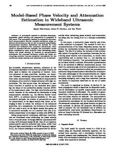
C

Correlator Structure for Separable Normalized Convolution

: uu uu 5 u uu jj ujujjjjj / 1 TTT ··I IIIITTTTT) II · II I$ ··· ·· · ··· p7 · ppp p ··· p pp e2 eYpeYeeeee ··· x Y Y Y N B NNN YYY, · NNN ¦¦ ¦ ··· NN' ¦ ¦ ·· ¦ ¦ · ¦¦ ··· ¦¦¦ 5 ¦ jjjj j ··¦¦ j j / x2 jT / c 6C TTTT 6C6CC TTT) 66 CC 66 CCC 66 CC 66 C! eee2 66 x3 YeeYeYeYe Y YYY, 66 66 ½ / x4

89:; ?>=