Spatial Filter Subspace Optimization Based on Mutual ...

Spatial Filter Subspace Optimization Based on Mutual Information Xinyang Li, Cuntai Guan, Kai Keng Ang and Haihong Zhang Institute for Infocomm Research (I2R) Agency for Science, Technology and Research (A*STAR) 1 Fusionopolis Way, 21-01 Connexis (South Tower) Singapore 138632 Email:{lixiy,ctguan,kkang,hhzhang}@i2r.a-star.edu.sg Abstract—Discriminating EEG signals between different motor imagery states is an important application of brain computer interface (BCI). However, low signal-to-noise ratio and significant data variation of EEG make it very difficult for BCI to obtain reliable results. Spatial filtering is one of the most successful feature extraction methods, and many efforts have been made to construct spatial filters that are robust against the data nonstationarity. In this paper, we propose a novel spatial filter optimization method based on mutual information which is estimated by Gaussian functions instead of Parzen window. We analyze the relationship between the mutual information and feature distance using a simulation study to show that optimization based on mutual information can contribute to feature stationarity. Moreover, we also evaluate the proposed method on a real world motor imagery EEG data set recorded from 16 subjects performing motor imagery or staying in idle state. The experimental results validate the effectiveness of the proposed spatial filter optimization method as it outperforms both the common spatial pattern analysis and filter-bank common spatial pattern analysis.

I. I NTRODUCTION Spatial filtering technique is very successful in extracting EEG features for BCI, as it enhances the poor spatial resolution of EEG. Among the spatial filtering methods, common spatial pattern analysis (CSP) is the most widely applied optimization method, especially in discriminating motor imagery EEG [1]. In CSP, spatial filters are optimized by maximizing the Rayleigh quotient between the average covariance matrices from two different classes, which is equivalent to the ratio of powers of the EEG signals from the two classes after spatial filtering. To improve CSP, many efforts have been made to combine temporal analysis with the spatial pattern analysis in CSP. In [2], common spatio-spectral pattern (CSSP) is proposed by optimizing spatial filters by adding a one-time-delayed sample, which means that the number of the channels is increased. In [3], common sparse spectral spatial pattern (CSSSP) extends CSSP by implementing the optimization of a complete global spatial-temporal filter into the objective function of CSP. In [4], iterative spatio-spectral patterns learning (ISSPL) is proposed, where spatio-spectral filters and the classifier are calculated sequentially from labeled multichannel EEG data in an iterative manner using both Rayleigh quotient and SVM as optimization functions. In [5], the temporal causal information

978-1-4673-7218-3/15/$31.00 ©2015 IEEE

has been addressed by jointly optimizing both the spatial filters and time-lagged coefficient matrices in a convolutive model. In addition to the optimization of a single frequency band, in [6], the authors propose discriminative filter bank CSP (DFBCSP), where the finite impulse response (FIR) filters and the associated spatial weights are also obtained in an iterative manner by optimizing Rayleigh quotient. Rather than using Rayleigh quotient, in the optimum spatio-spectral filtering network (OSSFN), the bandpass filters and spatial filters are jointly optimized to maximize the mutual information between feature vector variables and the class label [7]. Instead of optimizing global temporal or spatial filters, the the mutual information has been applied for discriminating EEG in a “soft” optimization manner. In [8], [9], [10], [11], EEG signals are filtered by multiple frequency bands, which are chosen to cover the most discriminative frequency range for the task of interest. In [8], [9], the multiple bandpass filters are denoted as a filter bank, for each filter band of which the spatial filters are obtained simply using CSP. Thus, each pair of bandpass and spatial filter yields CSP features that are specific to the frequency range of the bandpass filter. After calculation of features of each band, feature selection based on mutual information is applied. As a result of the feature selection, both spatial and temporal filters are optimized. Compared to the iterative joint optimization of temporal and spatial filters, the computational complexity of such “soft” optimization is lower. Besides joint spatial-temporal study, a number of algorithms approach to model generalization for feature extraction from the robust modelling perspective [?]. By adding certain terms to the denominator of the CSP objective function in the Rayleigh coefficient form, the regularization method has been widely used to enhance the robustness of the spatial filters. When firstly proposed in [12], the regularization-based robust model is denoted as invariant CSP (iCSP), where disturbance covariance matrices are calculated from prior physiological knowledge or extra measurements like EOG or EMG. However, the extra recordings or prior knowledge about noise are not always available or reliable. In [13], stationary CSP is proposed to obtain invariant CSP that is independent of additional recordings to estimate the nonstationary artefacts. In stationary CSP, nonstationarity is estimated as the sum of

ICICS 2015

absolute differences between the mean variance and variance of a certain trial in the projected space. By penalizing the crosstrial differences, spatial filters can keep the power features as consistent as possible across trials while differentiating the two conditions. In [14], the authors introduce a different penalizing term that measures the Kullback-Leibler divergence (KL-divergence) of distributions of EEG data across trials, and subsequently, the learning algorithm can minimize within-class dissimilarities while maximizing inter-class separation. In [15], the nonstationary projection directions are estimated based on the principal component analysis (PCA) using cross-subject data, and then penalized in the objective function to build subject-specific spatial filters. Similarly to [15], cross-subject data are also used in [16] to enhance the robustness of the spatial filters. In particular, instead of estimating the directions of the nonstationary components, average covariance matrices of multiple subjects are directly incorporated in the denominator of the Rayleigh coefficient as a kind of ground truth of the covariance matrix estimate. In this way, an inaccurate model could be avoided when only very few EEG data from a single subject are available. In [17], those methods regularizing nonstationarity measurements are unified in a divergence-based framework, and it is proved in [17] that spatial filters in CSP project the EEG data into subspaces where the KL-divergence between the data distributions from two classes is maximized. Therefore, the objective function of CSP can also be formed in a divergence-based framework. The significance of this work lies in the fact that it is a unified framework for CSP with different kinds of regularization. In our previous work, mutual information is used to optimize the weights of spatial filters given a set of spatial filter subspace [7]. However, the limitation of optimizing weights of spatial filters is that it yields spatial filters that are not entirely independent of each other. To address this issue, in this work, we propose to optimally construct the subspace of spatial filters with mutual information as objective functions so that the resultant spatial filters are orthogonal after the optimization. In [7], one of the reasons that weights of spatial filters are optimized instead of spatial filter subspace is the heavy computational burden of gradient calculation with respect to the mutual information objective function. To reduce the computational complexity, in this work, we adopt a simplified mutual information calculation rather than using the Parzen window [7], [8], [9]. The performance of the simplified mutual information calculation has been discussed and compared with that of using the Parzen window. Moreover, when firstly adopted in FBCSP, mutual information is used as a criterion to select the most discriminative features [8], [9]. Despite its effectiveness in feature selection, the function of mutual information in robust modelling has not been sufficiently investigated. Thus, in this work, we analyze the role that mutual information plays in feature stationarity. Based on the above discussion, we highlight the contributions of this paper as follows: (i) a mutual information based spatial filter subspace optimization method is proposed; and

(ii) the relationship between the mutual information and feature stationarity is discussed. II. F EATURE E XTRACTION WITH S PATIAL F ILTERING A. Common Spatial Pattern Analysis Given the bandpass filtered EEG data, 𝑋 ∈ R𝑛𝑐 ×𝑛𝑡 , that is recorded from 𝑛𝑐 electrodes with 𝑛𝑡 number of time sample points, the average covariance matrix for class 𝑐 can be obtained as 1 ∑ ¯𝑐 = 𝑅 𝑅𝑗 (1) ∣𝒬𝑐 ∣ 𝑐 𝑗∈𝒬

=

1 ∑ 𝑋𝑗 (𝑋𝑗 )𝑇 , 𝑐 ∈ {−, +} ∣𝒬𝑐 ∣ tr[𝑋𝑗 (𝑋𝑗 )𝑇 ] 𝑐

(2)

𝑗∈𝒬

where 𝑗 is the trial index and 𝒬𝑐 is the index set containing all trials belonging to class 𝑐. Then, the CSP spatial filter w is designed to maximize the variance of the spatially filtered signal under one condition while minimizing it under the other condition, which can be expressed by the following optimization problem: ¯ −/+ w𝑇 𝑠.𝑡. w(𝑅 ¯− + 𝑅 ¯ + )w𝑇 = 1 max w𝑅 w

(3)

Each of the solutions of (3) is one row of CSP projection matrix 𝑊 , which can also be decomposed as 𝑊 = 𝑈𝑇 𝑃

(4)

where 𝑃 is the whitening matrix such that ¯+ + 𝑅 ¯ − )𝑃 𝑇 = 𝐼 𝑃 (𝑅

(5)

¯ 𝑐 be the average covariance matrix after whitening, i.e., Let Σ ¯𝑐 = 𝑃𝑅 ¯𝑐𝑃 𝑇 Σ

(6)

𝑈 = [u1 , u2 , ..., u𝑚 ] in (4) is a matrix containing the eigen¯ 𝑐 that correspond to the largest and smallest vectors of Σ ¯ 𝑐 , and, subsequently, 𝑈 can be regarded as the eigenvalues of Σ discriminative subspace for feature extraction with 𝑚 as the dimension of feature. The covariance matrix after projection can be rewritten as Λ𝑗 = 𝑈 𝑇 Σ𝑗 𝑈

(7)

Σ𝑗 = 𝑃 𝑅 𝑗 𝑃 𝑇

(8)

where

Then, the feature vector for trial 𝑗 is f𝑗 = diag(Λ𝑗 )

(9)

which are the powers of the EEG signals after being projected by 𝑊 .

B. Mutual Information Objective Function In [8], [9], the mutual information objective function is used as a kind of soft-optimization. The mutual information is calculated for each feature dimension, and, subsequently, the spatial filters yielding the highest mutual information are selected. In this work, we propose to optimize the subspace 𝑈 to maximize the mutual information between class label variables 𝑐 and feature variable f, i.e., 𝐼(f, 𝑐)

(10)

= 𝐻(𝑐) − 𝐻(𝑐∣f)

𝐻(𝑐) is the entropy of the class label, i.e., ∑ 𝐻(𝑐) = 𝑝(𝑐) log2 𝑝(𝑐),

(11)

𝑐=+,−

and 𝐻(𝒞∣f) is the conditional entropy of the class label given the obtained feature vector 𝑚 1 1 ∑ ∑ ∑ (𝑝(𝑐∣f𝑗,𝑖 ) log(𝑝(𝑐∣f𝑗,𝑖 ))) (12) 𝐻(𝒞∣f) = − 𝑚 ∣𝒬𝑐 ∣ 𝑖=1 𝑐 𝑐=+,− 𝑗∈𝒬

The conditional probability of class 𝑐 given feature f𝑗,𝑖 , 𝑝(𝑐∣f𝑗,𝑖 ), can be computed as 𝑝(f𝑗,𝑖 ∣𝑐)𝑃 (𝑐) 𝑝(𝑐∣f𝑗,𝑖 ) = ∑ 𝑐=+,− 𝑝(f𝑗,𝑖 ∣𝑐)

(13)

where f𝑗,𝑖 , 𝑖 = 1, ..., 𝑚, is the 𝑖-th dimension feature of trial 𝑗. In [8], [9], the conditional probability of f𝑗,𝑖 given class 𝑐, 𝑝(f𝑗,𝑖 ∣𝑐), is estimated using Parzen window, as below 1 ∑ 𝑝(f𝑗,𝑖 ∣𝑐) = 𝑐 𝜑(f𝑗,𝑖 − f𝑘,𝑖 , ℎ𝑐𝑖 ) (14) ∣𝒬 ∣ 𝑐 𝑘∈𝒬

where ℎ𝑐𝑖 is a smoothing parameter for class 𝑐, and the 𝑖-th feature dimension. 𝜑 is a smoothing kernel given by 1 − ∣∣d∣∣ 𝑐2 (15) 𝜑(d, ℎ𝑐𝑖 ) = √ 𝑒 ℎ𝑖 2𝜋 In the optimization of 𝑈 , to perform the gradient search of 𝑈 with respect to 𝐼(f, 𝑐), we need to calculate the gradient of 𝑈 with respect to 𝑝(f𝑗,𝑖 ∣𝑐) in (14). To lower the computation complexity of calculating the gradient, we adopt a simplified way to estimate 𝑝(f𝑗,𝑖 ∣𝑐), as below 𝑝(f𝑗,𝑖 ∣𝑐)

= =

𝑐 𝜑(f𝑗,𝑖 − ¯f𝑖 , ℎ𝑐𝑖 ) 𝑐 𝑐 𝜑(d𝑗,𝑖 , ℎ𝑖 )

where d𝑐𝑗,𝑖 is the distance between f𝑗,𝑖 and smoothing parameter ℎ𝑐𝑖 can be calculated as ( )0.2 4 ℎ𝑐𝑖 = 𝜎𝑖𝑐 3∣𝒬𝑐 ∣

(16) ¯f𝑐 . 𝑖

And the

(17)

where 𝜎𝑖𝑐 is the standard deviation of f𝑘,𝑖 , 𝑘 ∈ 𝒬𝑐 . With (10) to (17), we optimize the subspace 𝑈 using the following optimization function ˆ = arg max 𝐼(f, 𝑐) 𝑈 𝑈

𝑠.𝑡. 𝑈 𝑇 𝑈 = 𝐼

(18)

The optimization is accomplished by a gradient descent on the manifold of orthogonal matrices, and details of the subspace approach can be found in [17], [18].

III. E XPERIMENTAL S TUDY A. Simulation Study In this section, we conduct a simulation study to investigate the relationship between feature distance and mutual information. Considering a set of 1-d feature, let the mean features of class + and − be 𝑓¯− 𝑓¯+

=

0.3

(19)

=

0.7

(20)

which is a typical pair of averaged CSP features given the constraint 𝑓¯− + 𝑓¯+ = 1 in the optimization objective function (3). Assuming that 𝑝(𝑐) = 0.5, we could calculate the mutual information information between the class variable 𝑐 and a 1-d feature 𝑓 , 𝐼(𝑓, 𝑐), by using (10) to (15). Define the relative distance 𝑑˜ as 𝑓 − 𝑓¯− 𝑑˜ = ¯+ ¯− (21) 𝑓 −𝑓

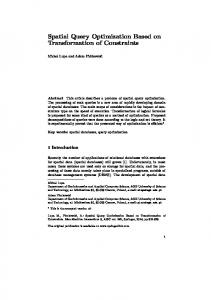
Thus, if 𝑑˜ = 0 feature 𝑓 is equal to 𝑓¯− and if 𝑑˜ = 1 feature 𝑓 is equal to 𝑓¯+ . With (21), we could investigate the change in mutual information with the change in 𝑑˜ under the assumption of different ℎ𝑐 in (15). The relationship between 𝑑˜ and 𝐼(𝑓, 𝑐) is illustrated in Figure 1. In Figure 1 (a), ℎ𝑐 in (15) are the same for both classes and the values are presented in the figure, and we can find that 𝐼(𝑓, 𝑐) is symmetric about 𝑑˜ = 0.5 and achieves the maximum value when 𝑑˜ = 0 or 𝑑˜ = 1. In other words, the less the feature distance 𝑑𝑐 , the higher the mutual information. Examples of 𝐼(𝑓, 𝑐) when ℎ𝑐 is not the same for the two classes are shown in Figure 1 (b) and (c). As shown by Figure 1 (b) and (c), although 𝐼(𝑓, 𝑐) is no longer symmetric, when 𝑑𝑐 is smaller, 𝐼(𝑓, 𝑐) is larger. Thus, generally speaking, by maximizing mutual information, the distance between a feature and the mean feature of one class could be minimized. As the calculation of mutual information is unsupervised, it cannot be guaranteed that the feature is closer to the center of the correct class. However, this could be advantageous as it makes the model less prone to over-fitting. B. Real World Motor Imagery Classification In this section, we evaluate the proposed method by a real world binary motor imagery EEG data set. 1) Data Collection Setup: 27-channel EEG were recorded by Nuamps EEG acquisition hardware with unipolar Ag/AgCl electrode channels, where a bandpass filter of 0.05 to 40 Hz was set. The sampling rate was 250 Hz with a resolution of 22 bits for the voltage range of ± 130 mV. In the experiment, the task is either motor imagery of dominant hand or idle state, and the training and test sessions were recorded on different days. During the EEG recording process, the subjects were instructed to avoid physical movement and eye blinking. Additionally, they were asked to perform kinaesthetic motor imagery of the chosen hand. During the idle state, they did mental counting to make the EEG signal more consistent. Each training session consisted

1.0

1.0

h− = 0.02, h+ = 0.05

0.6

0.4

0.6

0.4

0.2

h = 0.10

0.6

0.4

0.2

h− = 0.05, h+ = 0.10

h− = 0.10, h+ = 0.05

h− = 0.05, h+ = 0.50

h = 0.50 0.0 0.0

0.8 Mutual Information

Mutual Information

0.8

0.2

h− = 0.01, h+ = 0.05

h− = 0.05, h+ = 0.02

0.8 Mutual Information

1.0

h− = 0.05, h+ = 0.01

h = 0.01 h = 0.02

0.2

0.4

d˜

0.6

0.8

1.0

0.0 0.0

0.2

h− = 0.50, h+ = 0.05 0.4

(a)

d˜

0.6

0.8

0.0 0.0

1.0

0.2

0.4

(b)

d˜

0.6

0.8

1.0

(c)

Fig. 1. Mutual information as a function of 𝑑˜

3) Data Stationarity: To evaluate the feature stationarity, we adopt the KL-divergence which has been widely used for stationarity study in BCI [14], [15]. Because EEG data is usually processed to be centered, for two EEG data sets, 𝑗1 and 𝑗2 , the KL-divergence between them is

=

𝐷𝑘𝑙 (𝑅𝑗1 ∣∣𝑅𝑗2 ) ( ( ) ) det 𝑅𝑗1 1 −1 − 𝑛𝑐 (22) tr ((𝑅𝑗2 ) 𝑅𝑗1 ) − ln 2 det 𝑅𝑗2

𝑗∈𝒬

𝑐={+,−}

Figure 2 illustrates the comparison of Δ𝑠 between CSP and the proposed method for 9 filter bands, by applying the corresponding project matrices for the EEG signals filtered by each bandpass filter. Subfigures (a) and (b) correspond to the training and test data, respectively, where the x-axis represents the starting frequency of each bandpass filter and y-axis represents Δ𝑠 for the two methods. As shown by Figure 2, for both the training and test data and almost 9 frequency bands, average within-class KL-divergence, i.e., Δ𝑠 , is lower when the proposed method is applied. Thus, it can be seen that the data spatially filtered by the proposed method are more stationary. 0.90

Within-class KL-divergence

2) Classification Results: In Table I, we show the classification results of evaluating the spatial filter optimization methods proposed in Section II-B. For the single band setting, we compare the proposed spatial filter optimization method, indicated as “MI𝑠 ”, with CSP as the baseline, and both methods are applied to EEG signals filtered by one broad band 4 − 40𝐻𝑧. The obtained features are classified by the linear discriminant classifier (LDA). As shown in Table I, the proposed spatial filter optimization method outperforms single band CSP. To validate using (15) and (16) to calculate mutual information, we also use it to select features generated by the proposed optimization method for the multiple filter setting, and compare it with FBCSP where feature selection is based on Parzen window. 9 temporal bandpass filters, 4 − 8, 8 − 12, ..., 36 − 40𝐻𝑧 are constructed, as they are proved to cover the frequency range with the most distinctive eventrelated (de)synchronization (ERD/ERS) effects [8], [9]. For the two spatial filter optimization methods, 2 pairs of the spatial filters are used for each band. Thus, totally 36 features are obtained, for which feature selection is applied using mutual information based on different mutual information calculation methods. The comparison of classification results between the proposed method and FBCSP are also summarised in Talbe I. As shown by the results, the proposed spatial filter optimization method with the simplified mutual information for feature selection yields better results compared to FBCSP, which validate the effectiveness the objective function proposed in Section II-B.

where 𝑅𝑗1 and 𝑅𝑗2 are the covariance matrices of data sets 𝑗1 and 𝑗2 , respectively, Thus, the average within-class KLdivergence can be calculated as follows ∑ 1 ∑ 𝐷𝑘𝑙 (𝑊 𝑅𝑗 𝑊 𝑇 ∣∣𝑊 𝑅𝑐 𝑊 𝑇 ) (23) Δ𝑠 = ∣𝒬𝑐 ∣ 𝑐

CSP MIs

0.85 0.80 0.75 0.70 0.65 0.60 0

5

10

15 20 25 Frequence (Hz)

30

35

40

(a) 0.74

CSP MIs

0.72 Within-class KL-divergence

of 2 runs while the test session consisted of 2-3 runs. Each run lasted for approximately 16 minutes and comprised 40 trials of motor imagery and 40 trials of rest state. Details of the data collection and experiment setting can be found in [19].

0.70 0.68 0.66 0.64 0.62 0.60 0

5

10

15 20 25 Frequence (Hz)

30

35

40

(b) Fig. 2. Comparison of within-class KL-divergence

TABLE I F EATURE SELECTION CLASSIFICATION RESULTS USING FILTER BANK (%)

Subject 1 2 3 4 5 6 7 8 9 10 11 12 13 14 15 16 mean

Single Training Acc. CSP MI𝑠 84.375 83.125 64.167 80.833 63.333 90.833 87.500 88.333 90.000 90.833 90.833 90.833 78.333 78.333 78.333 78.333 88.750 89.375 68.333 73.333 68.333 73.333 90.833 91.667 66.875 66.875 90.000 91.250 73.750 85.000 85.000 88.750 79.806 84.208

Band Test Acc. CSP MI𝑠 57.083 57.500 50.417 57.500 51.250 56.250 52.500 52.083 50.833 51.667 65.000 64.583 70.000 70.417 70.000 70.417 72.500 71.250 55.833 61.667 55.833 61.667 81.250 80.417 50.417 50.417 70.000 75.000 70.417 65.417 70.000 74.167 62.667 64.111

IV. C ONCLUSION For practical BCI systems, how to construct a discriminative model that is robust against the data nonstationarity is one of the most challenging issues in spatial filter design. In this work, we proposed a novel spatial filter subspace optimization method based on mutual information. Due to the complexity of calculating mutual information based on Parzen window, in this work, we used the Gaussian functions centered at mean features of different classes to estimate the mutual information. To investigate the relationship between mutual information and feature stationarity, we conducted a simulation study which shows that by maximizing the mutual information within-class feature distances could be reduced. The effectiveness of the proposed spatial filter optimization method was evaluated by a real world motor imagery EEG data set. The classification results showed that the proposed method yielded accuracy improvements for both the single band and filter bank settings. R EFERENCES [1] Z. J. Koles, “The quantitative extraction and toporraphic mapping of the abnormal components in the clinical EEG,” Electroencephalography and Clinical Neurophysiology, vol. 79, pp. 440–447, 1991. [2] S. Lemm, B. Blankertz, G. Curio, and K.-R. M¨uller, “Spatio-spectral filters for improving the classification of single trial EEG,” IEEE Transactions on Biomedical Engineering, vol. 52, no. 9, pp. 1541 –1548, sept. 2005. [3] G. Dornhege, B. Blankertz, M. Krauledat, F. Losch, G. Curio, and K.-R. M¨uller, “Combined optimization of spatial and temporal filters for improving brain-computer interfacing,” IEEE Transactions on Biomedical Engineering, vol. 53, no. 11, pp. 2274–2281, nov. 2006. [4] W. Wu, X. Gao, B. Hong, and S.i Gao, “Classifying single-trial EEG during motor imagery by iterative spatio-spectral patterns learning (ISSPL),” IEEE Transactions on Biomedical Engineering, vol. 55, no. 6, pp. 1733–1743, June 2008. [5] X. Li, H. Zhang, C. Guan, S. H. Ong, K. K. Ang, and Y. Pan, “Discriminative learning of propagation and spatial pattern for motor imagery EEG analysis,” Neural Computation, vol. 25, no. 10, pp. 2709– 2733, 2013. [6] H. Higashi and T. Tanaka, “Simultaneous design of fir filter banks and spatial patterns for EEG signal classification,” IEEE Transactions on Biomedical Engineering, vol. 60, no. 4, pp. 1100–1110, April 2013.

Filter Bank Training Acc. Test Acc. FBCSP MI𝑠 FBCSP MI𝑠 80.625 90.000 50.417 64.167 89.167 90.833 60.417 58.750 84.167 90.833 52.917 60.833 94.167 91.667 71.250 63.750 95.000 92.500 58.750 59.167 97.500 97.500 83.333 82.500 97.500 95.000 78.750 77.083 98.333 98.333 96.250 89.583 94.375 95.000 69.167 70.000 85.000 92.500 65.000 63.333 69.167 90.833 51.250 56.667 92.500 93.333 79.583 80.833 73.125 73.750 49.583 49.167 90.625 93.125 75.000 70.000 91.875 95.625 62.917 62.083 90.625 89.375 71.667 69.167 88.875 92.056 66.972 67.194

[7] H. Zhang, Z. Y. Chin, K. K. Ang, C. Guan, and C. Wang, “Optimum spatio-spectral filtering network for brain-computer interface,” IEEE Transactions on Neural Networks, vol. 22, no. 1, pp. 52–63, Jan 2011. [8] K. K. Ang, Z. Y. Chin, C. Wang, C. Guan, and H. Zhang, “Filter bank common spatial pattern algorithm on BCI competition IV datasets 2a and 2b,” Frontiers in Neuroscience, vol. 6, no. 39, 2012. [9] K. K. Ang, Z. Y. Chin, H. Zhang, and C. Guan, “Mutual informationbased selection of optimal spatial-temporal patterns for single-trial EEGbased BCIs,” Pattern Recognition, vol. 45, no. 6, pp. 2137–2144, 2012. [10] K. P. Thomas, C. Guan, C. T. Lau, A. P. Vinod, and K. K. Ang, “A new discriminative common spatial pattern method for motor imagery braincomputer interfaces,” IEEE Transactions on Biomedical Engineering, vol. 56, no. 11, pp. 2730 –2733, Nov. 2009. [11] Q. Novi, C. Guan, T. H. Dat, and P. Xue, “Sub-band common spatial pattern (SBCSP) for brain-computer interface,” in the 3rd International IEEE/EMBS Conference on Neural Engineering, May 2007, pp. 204– 207. [12] B. Blankertz, M. Kawanabe, R. Tomioka, F. U. Hohlefeld, V. Nikulin, and K.-R. M¨uller, “Invariant common spatial patterns: Alleviating nonstationarities in brain-computer interfacing,” Advances in Neural Information Processing Systems, vol. 20, pp. 113–120, 2008. [13] W. Samek, C. Vidaurre, K.-R. M¨uller, and M. Kawanabe, “Stationary common spatial patterns for brain-omputer interfacing,” Journal of Neural Engineering, vol. 9, no. 2, pp. 026013, March 2012. [14] M. Arvaneh, C. Guan, K. K. Ang, and C. Quek, “Optimizing spatial filters by minimizing within-class dissimilarities in electroencephalogrambased brain computer interface,” IEEE Transactions on Neural Networks and Learning Systems, vol. 24, no. 4, pp. 610–619, June 2013. [15] W. Samek, F.C. Meinecke, and K.-R. M¨uller, “Transferring subspaces between subjects in brain-computer interfacing,” IEEE Transactions on Biomedical Engineering, vol. 55, no. 3, pp. 902–913, March 2008. [16] H. Lu, H. Eng, C. Guan, K. N. Plataniotis, and A. N. Venetsanopoulos, “Regularized common spatial pattern with aggregation for EEG classification in small-sample setting,” IEEE Transactions on Biomedical Engineering, vol. 57, no. 12, pp. 2936–2946, 2010. [17] W. Samek, M. Kawanabe, and K.-R. M¨uller, “Divergence-based framework for common spatial patterns algorithms,” IEEE Reviews in Biomedical Engineering, vol. 7, pp. 50–72, 2013. [18] M. D. Plumbley, “Geometrical methods for non-negative ica: Manifolds, lie groups and toral subalgebras,” Neurocomputing, vol. 67, pp. 161 – 197, 2005. [19] K. K. Ang, C. Guan, C. Wang, K. S. Phua, A. H. G. Tan, and Z. Y. Chin, “Calibrating EEG-based motor imagery brain-computer interface from passive movement,” 2011 Annual International Conference of the IEEE on Engineering in Medicine and Biology Society, EMBC, pp. 4199–4202, 2011.