c Statistical Research and Training Center ⃝ J. Statist. Res. Iran 10 (2013): 125–141
١۴١–١٢۵ ﺻﺺ،١٣٩٢ ﭘﺎﯾﯿﺰ و زﻣﺴﺘﺎن،٢ ﺷﻤﺎرهی،١٠ دورهی
Spatial Latent Gaussian Models: Application to House Prices Data in Tehran City Z. Ghayoumi, M. Mohammadzadeh∗ and K. Gholizadeh Tarbiat Modares University
Abstract. Latent Gaussian models are flexible models that are applied in several statistical applications. When posterior marginals or full conditional distributions in hierarchical Bayesian inference from these models are not available in closed form, Markov chain Monte Carlo methods are implemented. The component dependence of the latent field usually causes increase in computational time and divergence of algorithms. In this paper, an integrated nested Laplace approximation is used to solve these problems, in which the Laplace approximation and the numerical integration methods are combined in an efficient way so that hard simulations are replaced by fast computation and accurate approximation. Finally the relationship between house price data, floor size, age, number of rooms, building frame, type of proprietorship and facilities such as electricity, landline, water, gas, central heating and cooling system, kitchen goods, bath and toilet are modeled by using spatial latent Gaussian models. The fitted model can be used for predicting the house price in Tehran city. Keywords. Latent Gaussian model; Gaussian Markov random field; integrated nested Laplace approximation; Bayesian approach. MSC 2010: 62F15, 60G60, 44A10. ∗
Corresponding author
126
Spatial Latent Gaussian Models: Application to House Prices · · ·
1 Introduction Many researchers in various contexts need to achieve fast and accurate results, so new methods of calculations are required to fit complex models. The class of structured additive regression models introduced by Fahrmeir and Tutz (2001) are flexible and extensive, including: generalized linear models, generalized additive models, smoothing spline models, state space models, semi parametric regression models, and spatial and spatio-temporal models. In these models the response variable is assumed to belong to an exponential family, in which its mean is linked to some structured additive predictors. Latent Gaussian models are a perfect subclass of structured additive regression models that are used in several statistical applications, including (a) Regression models such as Bayesian generalized linear models (Dey et al., 2000), penalized spline models (Lang and Brezger, 2004) random-walk models (Rue and Held, 2005) and Gaussian processes (Chu and Ghahramani, 2005). (b) Dynamic models (West and Harrison, 1997) in which temporal dependence can be considered by using a covariate or a spatio-temporal covariance function. Finally, (c) spatial and spatio-temporal models (Banerjee et al., 2008). In these models spatial dependence can be modeled similarly, using a spatial covariate. Any two spatial and temporal dependencies can be achieved by using a spatio-temporal covariate or a spatio-temporal covariance function. The common approach of analyzing these models and obtaining the posterior marginals is the application of Monte Carlo Markov Chain (MCMC) algorithms. MCMC methods perform poorly when applied to such models because of the strong dependence among the components of latent field and the components of hayperparameter vectors, especially when the dimension of latent field is large. The Integrated Nested Laplace Approximation (INLA) is an approach proposed by Rue et al. (2009) to solve these problems, in which Laplace approximation and the numerical integration methods are combined in an efficient way, so that hard simulations are replaced by the fast computation and accurate approximations. Martino and Rue (2010) presented series of case studies running from generalized linear models to spatially varying regression models and survival models, solved by using INLA methodology. Martino et al. (2011) solved the problem of inference for some Stochastic Volatility models by applying INLA. Baghishani et al. (2012) introduced data cloning method for computing maximum likelihood estimates in complex statistical models. Ghayoumi et al. (2012) showed the applic 2013, SRTC Iran ⃝
Z. Ghayoumi, M. Mohammadzadeh and K. Gholizadeh
127
cation of INLA on the data set of childhood undernutrition in Zambia by using spatial latent Gaussian models. Muff et al. (2013) extended the INLA approach to formulate Gaussian measurement error models in GLM models. Gholizadeh et al. (2013) analyzed the crime Data in Tehran city using INLA. Gelfand et al. (2007) illustrated the use of multivariate models with spatially changeable coefficients on a data set obtained from the Singapore housing market. Rivaz (2012) analyzed the rent house data of Tehran city based on Bayesian and classical approaches by using Gaussian Markov Random Field. Khalili and Nobahar (2012) predicted the house price data in Tabriz city using Artificial Neural Network and Hedonic models. In this paper, the spatial latent Gaussian model (SLGM), its features and INLA method are briefly introduced. Then the applications of the SLGM by using INLA method are illustrated on the house price data set in Tehran city. Next the most suitable model is selected from the proposed models by common criteria. Finally, discussion and results are presented.
2 Model Description Suppose yi , i ∈ In is an observation of a response variable y related to a set of covariates, where In is an irregular lattice with n nodes in R2 . Latent Gaussian models are a perfect and flexible class of models that mean of response variable, that is, µi = E(yi ) is linked to a structured additive predictor, that is, ηi through a link function, namely g(·), so that g(µi ) = ηi . The structured additive predictor ηi accounts for effects of various covariates as ηi = α +
nf ∑
f j (uji ) +
j=1
nβ ∑
βk wki ,
i ∈ In
(1)
k=1
where {fj (·)}s are unknown functions of the covariates ui = (u1i , . . . , unj i ) and {βk }s represent the linear effect of covariates wi = (w1i , . . . , wnβ i ). The unknown functions {fj (·)} enable to provide any type of dependency such as temporal, spatial and spatio-temporal dependencies. Assume that the latent field x = (α, f1 , . . . , fnf , β1 , . . . , βnβ ) follows the Gaussian distribution with zero mean and precision matrix Q = Σ−1 , where Σ is the covariance matrix. The distribution of the n observational variables y = {yi : i ∈ In } is denoted by π(y|x, θ). Suppose y is conditionally independent given (x, θ) and assign Gaussian priors to α, {fj (·)} and {βk }. Then the joint posterior density of J. Statist. Res. Iran 10 (2013): 125–141
128
Spatial Latent Gaussian Models: Application to House Prices · · ·
the latent field x and m-dimensional hyperparameter vector θ is given by ∏ π(x, θ | y) ∝ π(θ)π(x | θ) π(yi | xi , θ) i∈I
[
] ∑ 1 T ∝ π(θ)|Q| exp − x Qx + log{π(yi | xi , θ)} . 2 n 2
i∈I
Latent Gaussian models often have two basic features. The first is that the latent Gaussian field x, which often have large dimension, holds the local, global and pairwise Markov properties (Rue and Held, 2005). Thus this latent field is a Gaussian Markov Random Field (GMRF) with sparse precision matrix Q. Hence, the numerical methods of sparse matrices can be used, which are faster than the methods served for dense matrices. The second is that the number of hyperparameters is small, e.g. less than 6. These two properties create the necessary conditions for fast inference (Eidsvik et al., 2009).
3 Gaussian Markov Random Field An undirected graph G is a double G = (V, ε), where V is a set of nodes, ε is a set of edges {i, j}, i, j ∈ V and i ̸= j. When V = {1, . . . , n}, the graph is called labeled. A random vector x = (x1 , . . . , xn )T ∈ R is called a GMRF with respect to a labeled graph G = (V, ε) with mean µ and precision matrix Q, if its density has the following form { } 1 n 1 π(x) = (2π)− 2 |Q| 2 exp − (x − µ)T Q(x − µ) 2 where Qij ̸= 0 ⇐⇒ {i, j} ∈ E
for all
i ̸= j.
Suppose Q is an n × n symmetric positive semi definite matrix with rank n − k > 0. Then x = (x1 , . . . , xn )T is an improper GMRF of rank n − k with parameters (µ, Q) if its density is given by { } −(n−k) 1 1 T ∗ ) ( π(x) = (2π) 2 (|Q| ) 2 exp − (x − µ) Q(x − µ) 2 where | · |∗ denotes the generalized determinant. A special type of GMRF is Intrinsic GMRF (IGMRF), which is always improper i.e. its precision matrix c 2013, SRTC Iran ⃝
Z. Ghayoumi, M. Mohammadzadeh and K. Gholizadeh
129
is not full rank. An IGMRF of rank n−k is an improper GMRF with feature QS k−1 > 0, where S k−1 is the polynomial design matrix (Rue and Held, ¯ 2005). These type of fields can be used quite extensively as smooth prior distribution in various applications, for example, the random walk models are a type of these priors. An IGMRF of second order x is called the second order Random Walk (RW2) because its second order increments are independent with normal distribution, that is, ∆2 xi = xi − 2xi+1 + xi+2 ∼N (0, κ−1 ), iid
i = 1, · · · , n − 2.
4 Integrated Nested Laplace Approximation Assume x = (α, f1 , . . . , fnf , β1 , . . . , βnβ ) is the latent random field. The posterior marginals of interest can be written as ∫ π(xi |y) = π(xi |y, θ)π(θ|y)dθ, i = 1, . . . , n, ∫ π(θj |y) = π(θ|y)dθ −j , j = 1, . . . , ℓ where θ −j denotes the vector θ with leaving its jth element out. The approximations of the posterior marginals returned by INLA have the following form ∑ π e(xi |y) = π e(xi |θ k , y)e π (θ k |y)∆k , i = 1, . . . , n, (2) ∫k π e(θj |y) =
π e(θ|y)dθ −j ,
j = 1, . . . , ℓ
(3)
where each π e(θ k |y) is the density value computed during an integrated schema on π e(θ|y), such as grid or Central Composite Design (CCD) strategy (Martino, 2007). The Laplace approximation used for the joint posterior of the hyperparameters, π(θ|y), is given by π eLA (θ|y) ∝
π(x, θ, y) | ∗ π eG (x|θ, y) x=x (θ )
(4)
where π eG (x|θ, y) is a Gaussian approximation to the full conditional of x at its mode for a given θ (Tierney and Kadane, 1986). Three options are available for π(xi |θ, y). The fastest option, πG (xi |θ, y), is the marginals of J. Statist. Res. Iran 10 (2013): 125–141
130
Spatial Latent Gaussian Models: Application to House Prices · · ·
the Gaussian approximation πG (x|θ, y) that is already computed when evaluating expression (4). The only extra cost to obtain π(xi |θ, y) is the computation of the marginal variances from the sparse precision matrix πG (x|θ, y) where they are computed using Takahashi’s equations (Takahashi et al., 1973). The Gaussian approximation often gives reasonable results, but the skewness of the distribution may not be captured by the Gaussian approximation (Rue and Martino, 2007). The more accurate approach would be used again a Laplace approximation, with a similar form to expression (4) that is given by π eLA (xi |θ, y) ∝
π(x, θ, y) | ∗ π eGG (x−i |xi , θ, y) x−i =x−i (xi ,θ )
(5)
where π eGG is the Gaussian approximation of πG (xi |xi , θ, y), x−i denotes all elements in x except its ith element and x∗−i (xi , θ) is the modal configuration. The third option, π eSLA (xi |θ, y) called simplified Laplace approximation is obtained by Taylor expansion on the numerator and denominator of (5) up to (s) i (θ) third order around xi = µi (θ). Setting xi = xiσ−µ , where µi (θ) and σi (θ) i (θ) are the mean and variance of the Gaussian approximation respectively, the expansions of the numerator and denominator in (5) are respectively given by 1 ( (s) )2 1 ( (s) )3 log{π(x, θ, y)} + x = − xi 2 6 i x−i =Eπ˜G (x−i |xi ) ∑ (3) dj {µi (θ), θ}{σi (θ)aij (θ)}3 + · · · × j∈ Iin
log{˜ πGG (x−i |xi , θ, y)}
x−i =Eπ˜G (x−i |xi )
∝ c0 +
1 log |Q∗ + diag(c)| 2
where Q∗ = Q[−i,−i] is the prior precision matrix of the GMRF with omit∂ 2 π(yj |xj ,θ ) ted ith column and row and ci = − |xj =Eπ˜ (x−j |xj ) . Then the ∂x2j G simplified Laplace approximation is defined as π ˜SLA (xsi |θ, y) = c0 −
1 ( (s) )2 1 ( (s) )3 (3) (1) (s) xi + γi (θ)xi + x γi (θ) + . . . 2 6 i c 2013, SRTC Iran ⃝
Z. Ghayoumi, M. Mohammadzadeh and K. Gholizadeh
131
where (1)
γi (θ) =
1 ∑ 2 σ (θ){1 − Corrπ˜G (xi , xj |θ)2 }d3j {(µi (θ), θ}σj (θ)aij (θ) 2 In j j∈
(3) γi (θ)
=
∑
i
(3)
dj {µi (θ), θ}{σi (θ)aij (θ)}3 .
j∈ Iin
In a simulation study, the authors showed that not only the results of INLA are much close to the results of MCMC, but also the calculation time by INLA is a quarter of calculation time with MCMC. Calculations were run on a computer with 33.3 GHz processor, 64 bit operating system and 12GB memory.
5
Evaluation Criteria
We use several criterions to compare different models and choose the most suitable. The first is Deviance Information Criterion (DIC), which is a measure of complexity and fit (Spiegelhalter et al., 2002). It compares complex hierarchical models, given by: DIC = D + pD where D is the posterior mean of the deviance and pD is the effective number of parameters. Small values of DIC indicate a good trade-off between complexity and fit of the model. Moreover, to compare models and detect outliers or surprising observations, the predictive measures (Pettit and Young, 1990) are used such as Conditional Predictive Ordinates (CPO) and Probability Integral Transforms (PIT). The conditional predictive ordinates are defined as: CP Oi = π(yi |y −i ), i ∈ In where the subscript in y −i indicates that the ith element of the vector y is removed. Unusually, small value of CP Oi indicates that yi is a surprising observation. The probability integral transform is defined as: P ITi = p(yinew 6 yi |y −i ),
i ∈ In
where its unusual large or small values indicate possible outliers. Furthermore, histogram of the PIT far from uniformity, might indicate a questionable model (Czado et al., 2007). Also to assess the predictive quality J. Statist. Res. Iran 10 (2013): 125–141
Spatial Latent Gaussian Models: Application to House Prices · · ·
0
0
5000
2000
10000
6000
15000
10000
20000
132
0
5000
10000
(a)
15000
20000
6
7
8
9
10
(b)
Figure 1. Histogram of price data (a): before transformation, (b): after transformation.
of the model the cross-validated logarithmic score defined by LogScore = −mean{log π(yi |y −i )} can be used. Also, in terms of Kullback-Leibler Distance (KLD) (Kullback and Leibler, 1951) we compare the approximation of the posterior distributions of parameters to original distribution. So, if KLD has a small value then the approximated distribution will be accurate.
6
Application
The aim of this section is analysis of the house price data of 22 regions of Tehran city with a SLGM by using INLA. The data set consists of information about 83970 residential units including 14 continuous, discrete and binary random variables including the location (22 regions of Tehran city), floor size (square meter), age, number of rooms, building frame, type of proprietorship, facilities such as electricity, landline, water, gas, central heating and cooling systems, kitchen, bath and toilet. According to the histogram of the data in Figure 1 (a) and the calculated p-value 2.2 × 10⁻¹⁶ for AndersonDarling normality test (Anderson and Darling, 1954), the price data does not follow a normal distribution. After using a logarithmic transformation on the response variable, its distribution becomes approximately normal that is shown in Figure 1 (b). Using Geary’C (Greay, 1954) with respect to H0 , lack of the spatial correlation, the spatial correlation test with p-value= 0.001 shows the significant spatial c 2013, SRTC Iran ⃝
Z. Ghayoumi, M. Mohammadzadeh and K. Gholizadeh
133
correlation of data. The approved spatial correlation of the price data is considered as a latent variable. Existence of old houses and the houses with large floor size in various regions may have different effects on the house prices and do not follow a consistent trend. So, considering random coefficients provides more flexible and more accurate model. Therefore, these two variables as latent variables and binary variables such as electricity, landline, water, gas, building frame, central heating and cooling systems, kitchen, bath and toilet as variables with fixed effects are considered. Let the transformed data be realizations of conditionally independent Gaussian random variables with unknown mean and precision λy . We consider three different models for the mean parameter, that is, ηi .
Model 1: The first model is defined as:
ηi = α + wTi β + fS (si ) + f1 (xi ) + roomi f2 (zi ),
i = 1, . . . , n
where w = (w1i , . . . , wnβ i ) is the vector of covariates to have linear effect and
β = (βelectrici , βphone , βwater , βgas , βheater , βcooler , βframe , βkitchen , βbath , βtoilet )
is the coefficients vector of w. This model contains a spatially structured component fS (si ), which is assumed to vary smoothly in regions. To account such smoothness, fS (si ) is modeled as an IGMRF with unknown precision λs . Also, f1 (xi ) and f2 (zi ) are the effects of year and floor size variables respectively, which are considered to be second-order random walk with unknown precision. The latent Gaussian random field of this model is x = {α, β, fS (·), f1 (·), f2 (·), ηi }, while the hyperparameters vector is θ = (λy , λs , λ1 , λ2 ). A vague independent Gamma (1, 5E−5) prior is assigned to each element of θ. Then the estimated coefficients along with their standard deviations, quartiles and KLDs are presented in Table 1. J. Statist. Res. Iran 10 (2013): 125–141
Spatial Latent Gaussian Models: Application to House Prices · · ·
−0.4
−0.2
0.0
0.2
134
10
20
30
40
Figure 2. Estimated effect of age in Model 1.
Table 1. Bayesian estimation of Model 1 parameters by using INLA Quantiles Covariate
Estimate
SD
0.025
0.975
KLD
µ
6.818
0.159
6.506
7.130
< 1E−45
βwater
0.022
0.012
0.000
0.044
< 1E−45
βgas
0.006
0.017
-0.028
0.041
3.7865E−29
βphone
0.027
0.007
0.013
0.041
5.42E−16
βelectrici
0.204
0.088
0.031
0.378
4.4231E−16
βbath
0.049
0.010
0.030
0.069
< 1E−45
βheater
0.034
0.004
0.025
0.043
1.116E−23
βcooler
0.034
0.005
0.025
0.044
< 1E−45
βkitchen
0.020
0.034
-0.047
0.086
2.319E−17
βframe
0.019
0.0002
0.019
0.020
< 1E−45
βtoilet
0.426
0.130
0.170
0.681
4.08E−16
Model 2: The estimated effect of age is displayed in Figure 2. Because the age variable has an approximately linear effect on the house price, so it is considered as a random effect variable. Hence, the previous model can be modified as ηi = α + wTi β + fS (si ) + roomi f1 (zi ). c 2013, SRTC Iran ⃝
135
0
0
1000
1000
2000
3000
3000
4000
5000
5000
Z. Ghayoumi, M. Mohammadzadeh and K. Gholizadeh
0.0
0.2
0.4
0.6
0.8
1.0
(a)
0.0
0.2
0.4
0.6
0.8
1.0
(b)
Figure 3. (a): Histogram of PITs of Model 1, (b): Histogram of PITs of Model 2.
Here the latent Gaussian field and hyperparameters vector are x = {α, β, fS (·), f1 (·), ηi } and θ = (λy , λs , λ1 ), respectively. The coefficients estimates of this model and their standard deviations, quartiles and KLD are summarized in Table 3. As shown in Table 2, DIC criterion of Model 1 is smaller than Model 2, this is because of the additional random effect in the model. Because pD value of Model 1 is also bigger, Model 2 is less complicated than Model 1. The histogram of PITs in Figure 3 (a) is not uniform for Model 1 while the histogram of Model 2 is almost uniform, which is shown in Figure 3 (b). Therefore Model 2 is more preferable than Model 1.
Table 2. Evaluation criteria of all models provided for house price data Criterion pD
DIC
LogScore
Calculation Time (minutes)
Model 1
54.61
110792.78
0.659
3.7497
Model 2
44.04
111317.95
0.663
2.2677
Model 3
46.62
111320.58
0.663
3.5092
Model 3: It seems that there is non-spatial correlation between areas, thus J. Statist. Res. Iran 10 (2013): 125–141
Spatial Latent Gaussian Models: Application to House Prices · · ·
136
by maintaining the overall form of previous model, Model 3 is defined as ηi = α + wTi β + fS (si ) + fU (ui ) + roomi f1 (zi ), where fU (ui ) is a spatially unstructured component which is normally distributed with zero mean an unknown precision λu . The latent Gaussian field of this model is x = {α, β, fS (·), fU (·), f1 (·), ηi }, while the hyperparameters vector is θ = (λy , λs , λu , λ1 ). The estimated coefficients, along with their standard deviations, quartiles and KLDs are given in Table 4.
Table 3. Bayesian estimation of Model 2 parameters by using INLA Quantiles Covariate
Estimate
SD
0.025
0.975
KLD
µ
6.533
0.160
6.219
6.846
< 1E−45
βwater
0.023
0.011
0.000
0.045
< 1E−45
βgas
0.035
0.017
0.000
0.069
< 1E−45
βphone
0.026
0.007
0.012
0.040
1.654E−24
βelectrici
0.200
0.089
0.025
0.374
8.272E−25
βbath
0.051
0.010
0.031
0.070
< 1E−45
βheater
0.032
0.004
0.023
0.041
< 1E−45
βcooler
0.036
0.004
0.026
0.046
4.5491E−24
βkitchen
0.022
0.034
-0.045
0.089
< 1E−45
βframe
0.019
0.0002
0.018
0.019
< 1E−45
βtoilet
0.408
0.131
0.151
0.664
8.112E−16
βage
0.021
0.0001
0.021
0.021
< 1E−45
According to Table 2, the values of pD , DIC and calculation time have increased for Model 3. Hence, adding a randomized component fU (ui ) has no desirable effect on the model accuracy. Therefore, among all the models, Model 2 is the best suitable one.
c 2013, SRTC Iran ⃝
137
0.096
0.098
0.100
0.102
0.104
0.106
Z. Ghayoumi, M. Mohammadzadeh and K. Gholizadeh
100
200
300
400
500
Figure 4. Estimated effect of the floor size in Model 2.
Table 4. Bayesian estimation of Model 3 parameters by using INLA Quantiles Covariate
Estimate
SD
0.025
0.975
KLD
µ
6.531
0.159
6.216
6.844
< 1E−45
βwater
0.023
0.011
0.000
0.045
4.099E−16
βgas
0.035
0.017
0.001
0.070
< 1E−45
βphone
0.026
0.007
0.012
0.041
< 1E−45
βelectrici
0.201
0.088
0.026
0.375
4.394E−16
βbath
0.051
0.009
0.031
0.070
< 1E−45
βheater
0.031
0.004
0.023
0.040
< 1E−45
βcooler
0.036
0.005
0.026
0.045
< 1E−45
βkitchen
0.022
0.034
-0.045
0.089
3.456E−16
βframe
0.019
0.0002
0.019
0.020
6.037E−13
βtoilet
0.408
0.130
0.151
0.664
< 1E−45
βage
0.021
0.0001
0.020
0.021
< 1E−45
Estimated effect of the size feature is displayed in Figure 4. It is clear that floor size has an incremental and non-linear effect on house price. The estimated spatial structure and the estimated standard deviation are illustrated in Figures 5. With respect to Figure 5 (a), the estimated spatial structure in the east J. Statist. Res. Iran 10 (2013): 125–141
Spatial Latent Gaussian Models: Application to House Prices · · ·
138
−0.0256
0
0.0277
0.005
(a)
0.0131
(b)
Figure 5. (a): Posterior mean for the spatial structure of the Model 2, (b): Standard Deviation of Model 2.
and center of Tehran is negative and in the west of city (regions 5 and 22) is positive. Also the map of estimated standard deviations, in Figure 5 (b), show appropriate accuracy of the predictions.
7 Discussion and Results Regarding spatial models, INLA as powerful inferential tool for latent Gaussian models has been used to tackle problems in analysis of lattice data, Geostatistics and point processes. In all cases, spatial dependency is modeled via the precision matrix of Gaussian random effects. However from a computational point of view, the normal assumption for latent variables is considered just for convenience in practice, but testing this assumption is impossible, which needs to be considered in future research. In this paper the latent Gaussian models are described and illustrated with its application on the house price data by using INLA. It is shown that Model 2 is the best among all three suggested models, that is why its DIC and LogScore are smaller than the others. Also, histogram of the PITs of Model 2 is almost uniform, so this model is suitable for prediction of house price in Tehran city. According to the results, studying 117 districts in Tehran instead of 22 regions with a priori assigned weighted Basage (Rue and Held, 2005), will result in a smoothed function. Moreover considering variables such as neighborhood security position, liquidity or building special facilities c 2013, SRTC Iran ⃝
Z. Ghayoumi, M. Mohammadzadeh and K. Gholizadeh
139
such as swimming pool, backyard, etc. would give more accurate models. Time trend also can be entered as a latent variable in model.
References Anderson, T.W. and Darling, D.A. (1954). A Test of Goodness-of-Fit, Journal of the American Statistical Association, 49, 765-769. Baghishani, H., Rue, H. and Mohammadzadeh, M. (2012). On a Hybrid Data Cloning Method and Its Application in Generalized Linear Mixed Models, Statistics and Computing, 22, 597613. Banerjee, S. Gelfand, A.E., Finely, A.O. and Sang, H. (2008). Gaussian Predictive Process Models for Larg Spatial Data Sets, Jornal of the Royal Statistical Society, Series B, 70, 825-848. Chu, W. and Ghahramani, Z. (2005). Gaussian Processes for Ordinal Regression, Journal of Machine Learning Research, 6, 1019-1041. Czado, C., Gneiting, T., and Held, L. (2007). Predictive Model Assessment for Count Data, Technical Report No. 518, University of Washington, Department of Statistics. Dey, D.K., Ghosh, S.K. and Mallick, B.K. (2000). Generalized Linear Models: A Bayesian Perspective. Boca Raton, Chapman and Hall, CRC. Eidsvik, J., Martino, S. and Rue, H. (2009). Approximation Bayesian Inference in Spatial Generalized Linear Mixed Models, Scandinavian Journal of Statistics, 36, 1-22. Fahrmeir, L. and Tutz, G. (2001). Multivariate Statistical Modeling Based on Generalized Linear Models, (2nd edn) Springer, Berlin. Geary, R.C. (1954). The Contiguity Ratio and Statistical Mapping, The Incorporated Statistician, 5, 115-145. Gelfand, A.E., Banerjee, S., Sirmans, C.F., Tu, Y. and Engong, S. (2007). Multilevel Modeling Using Spatial Processes: Apllication to the Singapore Housing Market, Science Direct, 51, 3567-3579. Gholizadeh, K., Mohammadzadeh, M. and Ghayoumi, Z. (2013). Spatial Analysis of Structured Additive Regression and Modeling of Crime Data in Tehran City Using Integrated Nested Laplace Approximation, Journal os Statistical Sciences, 7, 103-124. Khalili, A.M. and Nobahar, E. (2012). Predicting Housing Prices for the City of Tabriz: Application of the Hedonic Pricing and Artificial Neural Network Models, Journal of Economic Research and Policies, 60, 113-138.
J. Statist. Res. Iran 10 (2013): 125–141
140
Spatial Latent Gaussian Models: Application to House Prices · · ·
Kullback, S. and Leibler, R.A. (1951). On Information and Sufficiency, Anals of Mathematical Statistics, 22, 79-86. Lang, S. and Brezger, A. (2004). Bayesian P-splines, Journal of Computational and Graphical Statistics, 13, 183-212. Martino, S. (2007). Approximation Bayesian Inference for Latent Gaussian Models, Ph.D Thesis, Department of Mathematical Sciences, Norwegian University of Science and Technology, Trondheim. Martino, S. and Rue, H. (2010). Implementing Approximate Bayesian Inference Using Integrated Nested Laplace Approximation: A Manual for the INLA Program. Martino, S., Asa, K., Lindquist, O., Neef, L. and Rue, H. (2011). Estimating Stochastic Volatility Models Using Integrated Nested Laplace Approximations. The European Jornal of Finance, 7, 487-504. Muff, S., Riebler, A., Rue, H., Saner, P. and Held, L. (2013). Measurement Error in GLMMs with INLA, Statistical Science, Technical report at arxiv.org. Pettit, L.I. and Young, K.D. (1990). Measuring the Effect of Observation on Bayes Factors, Biomatrika, 77, 455-466. Rivaz, F. (2012). Analysis of the Gaussian Markov Random Field and its Application on the Sampling Schema of the House Rent and Price, Research Report, Statistical Research and Training Center, Tehran, Iran. Rue, H. and Held, L. (2005). Gaussian Markov Random Fields: Theory and Applications, Vol 104 of Monographs on Statistics and Applied Probability. Chapman & Hall, London. Rue, H. and Martino, S. (2007). Approximation Baysian Inference for Hierarchical Gaussian Markov Random Fields Moddels, Journal of Statistical Planning and Inference, 137, 31773192. Rue, H., Martino, S. and Chopin, N. (2009). Approximation Bayesian Inference for Latent Gaussian Models by Using Integrated Nested Laplace Approximations, Jornal of the Royal Statistical Society, Series B, 71, 319-392. Spiegelhalter, D.J., Best, N.G., Carlin, B.P., and van der Linde, A. (2002). Bayesian Measures of Model Complexity and fit. Journal Royal Statistical Society, Series B, 64, 583-639. Takahashi, K., Fagan, J. and Chen, M. (1973). Formation of a Sparse Bus Impedance Matrix and its Application to short Circuit Study, 8th PICA Conference Proceedings, Minneapolis, Minnesota, 177-179. Tierney, L. and Kadane, J. (1986). Accurate Approximations for Posterior Moments and Marginal Densities, Journal of the American Statistical Association, 81, 82-86. c 2013, SRTC Iran ⃝
Z. Ghayoumi, M. Mohammadzadeh and K. Gholizadeh
141
West, M. and Harrison, J. (1997). Bayesian Forecasting and Dynamic Models, 2nd edn. Springer, Berlin.
Z. Ghayoumi Department of Statistics, Tarbiat Modares University, Tehran, Iran. email:
[email protected]
K. Gholizadeh Department of Statistics, Tarbiat Modares University, Tehran, Iran. email:
[email protected]
J. Statist. Res. Iran 10 (2013): 125–141
M. Mohammadzadeh Department of Statistics, Tarbiat Modares University, Tehran, Iran. email: mohsen
[email protected]
c Statistical Research and Training Center ⃝ دورهی ،١٠ﺷﻤﺎرهی ،٢ﭘﺎﯾﯿﺰ و زﻣﺴﺘﺎن ،١٣٩٢ص ١۴٣
J. Statist. Res. Iran 10 (2013): 143
ﻣﺪلﻫﺎی ﮔﺎوﺳﯽ ﭘﻨﻬﺎن ﻓﻀﺎﯾﯽ :ﮐﺎرﺑﺮد در دادهﻫﺎی ﻗﯿﻤﺖ ﻣﺴﮑﻦ در ﺷﻬﺮ ﺗﻬﺮان زﻫﺮا ﻗﯿﻮﻣﯽ ،ﻣﺤﺴﻦ ﻣﺤﻤﺪزاده و ﮐﺒﺮی ﻗﻠﯽزاده داﻧﺸﮕﺎه ﺗﺮﺑﯿﺖ ﻣﺪرس
ﭼﮑﯿﺪه .ﻣﺪلﻫﺎی ﮔﺎوﺳﯽ ﭘﻨﻬﺎن ﻣﺪلﻫﺎی اﻧﻌﻄﺎفﭘﺬﯾﺮی ﻫﺴﺘﻨﺪ ﮐﻪ در زﻣﯿﻨﻪﻫﺎی ﮐﺎرﺑﺮدی ﻣﺘﻌﺪدی ﻣﻮرد اﺳﺘﻔﺎده ﻗﺮار ﻣﯽﮔﯿﺮﻧﺪ .ﮔﺎﻫﯽ در ﺗﺤﻠﯿﻞ ﺑﯿﺰ ﺳﻠﺴﻠﻪﻣﺮاﺗﺒﯽ اﯾﻦﮔﻮﻧﻪ ﻣﺪلﻫﺎ ﺗﻮزﯾﻊﻫﺎی ﭘﺴﯿﻨﯽ ﯾﺎ ﺷﺮﻃﯽ ﮐﺎﻣﻞ ﻓﺮم ﺑﺴﺘﻪای ﻧﺪارﻧﺪ ،ﻟﺬا ﺑﺮای ﻣﺤﺎﺳﺒﻪی آنﻫﺎ از اﻟﮕﻮرﯾﺘﻢﻫﺎی ﻣﻮﻧﺖ ﮐﺎرﻟﻮی زﻧﺠﯿﺮ ﻣﺎرﮐﻮﻓﯽ اﺳﺘﻔﺎده ﻣﯽﺷﻮد .وﺟﻮد ﻫﻤﺒﺴﺘﮕﯽ ﺑﯿﻦ ﻋﻨﺎﺻﺮ ﻣﯿﺪان ﭘﻨﻬﺎن ﻣﻌﻤﻮﻻ ﻣﻮﺟﺐ اﻓﺰاﯾﺶ زﻣﺎن ﻣﺤﺎﺳﺒﺎت و ﻧﺎﻫﻤﮕﺮاﯾﯽ اﯾﻦ اﻟﮕﻮرﯾﺘﻢﻫﺎ ﻣﯽﺷﻮد .در اﯾﻦ ﻣﻘﺎﻟﻪ ،ﺑﺮای ﺣﻞ ﻣﺸﮑﻼت ﻣﺰﺑﻮر ﺗﻘﺮﯾﺐ ﻻﭘﻼس آﺷﯿﺎﻧﯽ ﺟﻤﻊﺑﺴﺘﻪ اﺳﺘﻔﺎده ﻣﯽﺷﻮد ،ﮐﻪ در آن روشﻫﺎی اﻧﺘﮕﺮالﮔﯿﺮی ﻋﺪدی و ﺗﻘﺮﯾﺐ ﻻﭘﻼس ﺑﻪ ﻃﺮﯾﻘﯽ ﮐﺎرا ﺗﺮﮐﯿﺐ ﺷﺪه ﺑﻪﻃﻮری ﮐﻪ ﻣﺤﺎﺳﺒﺎﺗﯽ ﺳﺮﯾﻊ و ﺗﻘﺮﯾﺒﯽ دﻗﯿﻖ ﺟﺎﯾﮕﺰﯾﻦ ﺷﺒﯿﻪﺳﺎزیﻫﺎی ﺳﻨﮕﯿﻦ ﻣﯽﺷﻮد .ﻧﻬﺎﯾﺘﺎً راﺑﻄﻪی ﺑﯿﻦ دادهﻫﺎی ﻗﯿﻤﺖ ﻓﺮوش ﻣﺴﮑﻦ در ﺷﻬﺮ ﺗﻬﺮان و ﻣﺘﻐﯿﺮﻫﺎی ﻣﺴﺎﺣﺖ ،ﺳﻦ، ﺗﻌﺪاد اﺗﺎق و اﺳﮑﻠﺖ ﺳﺎﺧﺘﻤﺎن و ﻧﯿﺰ اﻣﮑﺎﻧﺎﺗﯽ ﻧﻈﯿﺮ ﺑﺮق ،آب ،ﮔﺎز ،ﺳﯿﺴﺘﻢ ﺣﺮارت و ﺑﺮودت ﻣﺮﮐﺰی، آﺷﭙﺰﺧﺎﻧﻪ ،ﺣﻤﺎم و ﺗﻮاﻟﺖ ﺑﺎ ﺑﮑﺎرﮔﯿﺮی ﻣﺪلﻫﺎی ﮔﺎوﺳﯽ ﭘﻨﻬﺎن ﻓﻀﺎﯾﯽ ﻣﺪلﺑﻨﺪی ﻣﯽﺷﻮد .ﻣﺪل ﺑﺮﺗﺮ ﻣﯽﺗﻮاﻧﺪ ﺑﺮای ﭘﯿﺸﮕﻮﯾﯽ ﻗﯿﻤﺖ ﻣﺴﮑﻦ در ﺷﻬﺮ ﺗﻬﺮان ﻣﻮرد اﺳﺘﻔﺎده ﻗﺮار ﮔﯿﺮد. واژﮔﺎن ﮐﻠﯿﺪی .ﻣﺪل ﮔﺎوﺳﯽ ﭘﻨﻬﺎن؛ ﻣﯿﺪان ﺗﺼﺎدﻓﯽ ﻣﺎرﮐﻮﻓﯽ ﮔﺎوﺳﯽ؛ ﺗﻘﺮﯾﺐ ﻻﭘﻼس آﺷﯿﺎﻧﯽ ﺟﻤﻊﺑﺴﺘﻪ؛ رﻫﯿﺎﻓﺖ ﺑﯿﺰی.
ﻧﺴﺨﻪی ﮐﺎﻣﻞ اﯾﻦ ﻣﻘﺎﻟﻪ ،ﺑﻪ زﺑﺎن اﻧﮕﻠﯿﺴﯽ در ﺻﻔﺤﻪﻫﺎی ١٢۵ﺗﺎ ١۴١آﻣﺪه اﺳﺖ.