Geo-spatial Information Science 14(3):157-163
Volume 14, Issue 3
DOI 10.1007/s11806-011-0522-z
September 2011
Article ID: 1009-5020(2011)03-157-07
Document code: A
Spatial Modeling Using High Resolution Image for Future Shoreline Prediction Along Junput Coast, West Bengal, India Abhisek Santra1,
D. Mitra2,
Shreyashi Mitra1
1. School of Geography, University of Southampton, University Road, Southampton, SO17 1BJ, Hampshire, UK 2. Indian Institute of Remote Sensing, NRSC-ISRO, 4 Kalidas Road, Dehradun 248001, Uttarakhand, India © Wuhan University and Springer-Verlag Berlin Heidelberg 2011
Abstract
National policies and legal decisions are very much dependent on the position of the shoreline. Shoreline change rates
are frequently employed to summarize historical shoreline movements. This also helps to predict the future position of the shoreline based on the perceived historical trends. In this regard, the future shoreline positions at both the long-term, that is 2050, and short-term, that is 2015, time interval was predicted using the End Point Rate (EPR) model along the Junput Coast of West Bengal, India. The whole project work was divided into five parts. The first part showed the detection of shoreline from satellite data like IRS LISS Ⅳ and Landsat 7 ETM+ and from the Survey of India Toposheet. The second part gave the glimpse of the dynamic segmentation of the shoreline to get the dynamically segmented nodal points along the shoreline. Shoreline prediction for the years 2015 and 2050 using End Point Rate (EPR) model was done in the third part. In the fourth part, Coastal Terrain Model (CTM) was prepared, and the digital shoreline estimated. The model result was validated and accuracy assessed with respect to the GPS data collected from the field at the fifth stage. Finally at the end of the present work, limitations of the project and the future scope of the work was sited. Keywords
end point rate model; dynamic segmentation; coastal terrain model
CLC number P237
Introduction The coastline or shoreline in general is the transitional boundary between land and sea water and is dynamic in nature. [1] The coastline is arguably the most important of all boundaries to be incorporated in the marine cadastre. It delineates the marine and terrestrial
environments and forms the basis for the generation of many local, state, national and international maritime limits. However, it must be underscored that the shoreline is very dynamic in nature. It undergoes regular changes, long term and short term, caused by hydro-dynamic changes (e.g. river cycles, sea-level rise), geomorphological changes (e.g. barrier island formation, spit development) and other factors (e.g.
► Received on February 22, 2011. ► Supported by Indian Institute of Remote Sensing (ISRO), India and ITC, the Netherlands. ► Abhisek Santra is a Ph.D. (Sc.) from University of Calcutta. He was a lecturer in the department of Geography of Syamaprasad College, University of Calcutta, India. After that he worked as a project manager on a joint GIS project conducted by NIC, Govt. of India and WBSMB, Govt. of West Bengal, India. Presently, he has been working on specializing his career in the applied domain of remote sensing and GIS through a post graduate program in the University of Southampton, UK. His areas of interests are radiometric normalization, digital image processing, geostatistics and spatial data analysis and modeling. ► E-mail:
[email protected]
158 Geo-spatial Information Science 14(3): 157-163
sudden and rapid seismic and storm events).[2]Our national policies and legal decisions are very much dependent on the position of shoreline. The study of the shoreline, and rate of change of shoreline is important for a wide range of coastal studies, such as development of setback planning, hazard zoning, erosionaccretion studies, regional sediment budgets and conceptual or predictive modeling of coastal morpho-dynamics. [3-5] Shoreline change rates are the frequency of shoreline movements used to predict the future position of the shoreline based on the perceived historical trends. There are several conventional techniques to determine the change rate of the shoreline position, including field measurement of the present water level, shoreline determination from aerial photography, topographical sheets and satellite imageries, comparison with the historical data using the End Point Rate (EPR) model,[6] Average of Rates (AOR), Linear Regression (LR) and Jack Knife (JK).[7] In the present study, the future probable shoreline position along the Junput coast of West Bengal, India was estimated from the historical data applying the EPR model.
1
Study area
The study area of the present research is the linear stretch of Junput coast along the Bay of Bengal between 21º 38' 53.33" N to 21º 46' 18.46" N and 87º 39' 25.96" E to 87º 49' 01.79" E. The total area is about 201.56 km2. This coastal part of the Bay of Bengal is famous for tourism and fishing purposes. Fig.1 shows the area of study. The beach material of the study area is generally siliciclastic and quartzo-felsperic in composition with well sorted medium to fine sand. In some parts silty sand and clayey sand dominate because of the riverine influence. The estuarine mud in many places mixes with beach sand creating mixed flats. A major portion of the mud is carried offshore, which constantly keeps the coastal water turbid. [8] Mudflats in some places make the shoreline inaccessible. Refering to the historical records of erosion and accretion, the western side of the Pichhabani inlet is erosion prone while the coast between the Pichhabani inlet
Fig. 1
Location of the study area
and Rasulpur River is marked as an accretional regime. Inside the coast, sand dunes of low height are prominent. C14 dating of the coast showed that this stretch of the beach is 2920±160 years old.[8] According to the bathymetric chart, the general off-shore gradient is 1:0.0025. This zone is characterized by a spectrum of surficial and internal sedimentary and biogenic structures.[9] Sediment is generally of a sandy type due to the riverine influences. The texture of the sediments varies mainly from silty sand to clayey sand along the coast. The grain size is relatively smaller in comparison to the normal sea beach sand particles. Porosity and permeability of the top sediment are much less than that of the interior sediments. Inside the coast, one can find silty and sandy loamy sediments where agriculture is practiced. The climate of the study area is of moderate type. The average annual temperature and rainfall are 28º C and 120 cm respectively. High velocity sea breeze is a characteristic feature of the area. Cyclones of different intensities normally come 2 to 3 times a year. These cyclonic storms are severe, with massive wave heights when they are accompanied by equinoxial tide. Those destructive waves (average height 5-6 m) devastate the coast. The huge waves topple all coastal physiographic barriers, including seawalls, groins and embankments and floods the inland areas behind the backshore. Seawalls were heavily destroyed in Junput and its immediate surrounding areas due to severe storms in 1987, 1997 and 2002.
Abhisek Santra, et al./ Spatial Modeling Using High Resolution … 159
This coastal strip of the Bay of Bengal belongs to a mesotidal (tidal amplitude of 2-4 m) to macro tidal ∨ 4 m), mostly at the eastern part) (tidal amplitude of regime with semi-diurnal tides with slight diurnal inequality. Wave climate is moderate in nature with an average height of 2-3 m but during cyclonic storms, wave height may reach up to 7 m. Heavy wind speeds along with those waves cause severe threats to the beach construction, tourism and fishing in this region, mainly at the erosional regime. Dune erosion leads to the landward retreat of the beach, lowering the beach profile and causing dune vegetation loss. Internal structures of the dunes, along with various crossbedded units, exhibit on the exposed face intercalated mud layers (5-15 m thick) at significant distances of 17 to 20 m from the shoreline. This indicates episodes of inundation of the dunes during catastrophic floods. [8] There are seasonal reversals of North-East winter to South-West summer winds, which play a significant role in transporting the dry sand of the sub-aerial beach, causing mobilization and remobilizing of dunes and the spilling of sand from the dunes to the inter-tidal zone. [10] This coastal stretch of Junput and its surrounding area is prone to both coastal erosion and accretion. Due to these factors, the shoreline has shifted from time to time and this shifting has influenced anthropogenic activity and settlement along the coast.
Fig. 2
2
Materials and methods
The dynamic coastline is important from both the natural and socio-economic points of view. Coastal managers, decision makers and local inhabitants need accurate and up-to-date information about shoreline changes due to erosion and accretion at regular time intervals. In this respect, remote sensing data and historical data have proved to be very effective. All these data have been used for mapping the shoreline position. For the past two and half decades remote sensing data coupled with historical data have been of great use as they produce a synoptic view and rhythmic coverage of the entire earth. For the present study, the following dataset was used: Survey of India toposheet of the year 1951 Bathymetric chart prepared by National Hydrographic Office (N.H.O) of India Shuttle RADAR Topography Mission (SRTM) data (GTOPO-30) Landsat-7 ETM+ image of the year 2000 IRS P6 LISS-Ⅳ image of the year 2006 The methodology adopted here was divided into five subdivisions, as shown (Fig.2).
General methodology
160 Geo-spatial Information Science 14(3): 157-163
Data pre-processing Dynamic segmentation of the shoreline Shoreline prediction Digital shoreline estimation Model validation In the data pre-processing phase, IRS P6 LISS-Ⅳ imagery was geo-referenced with the help of Landsat-7 ETM+ image with UTM, WGS-84, and zone 45 North projection systems. The toposheet was georeferenced in the same reference systems. While performing geo-referencing, the 1st order polynomial equation and nearest neighbor re-sampling technique were used. Generally, for moderate to less distortion in a relatively small area of an image, a first order polynomial transformation is sufficient to rectify the image to a geographic frame of reference. [11] Following the nature of the coastal stretch, the 1st order polynomial transformation was used. The nearest neighbor re-sampling approach was applied because of its simplicity and the ability to preserve original values in the unaltered image. [12] The toposheet was re-sampled at 28.5 m spatial resolution following the resolution of Landsat 7 ETM+ image. The higher spatial resolution of 5.8 m in IRS P6 LISS Ⅳ image was kept intact to retrieve a higher resolution coastal information. After sub-setting of the Area of Interest (AOI) the Landsat-7 ETM+ and LISS-Ⅳ images were further processed to extract the shoreline. False Colour Composite (FCC) of both the images was prepared by stacking the Green, Red and Near Infra Red bands. The shoreline was extracted by performing RGB to ISH (Intensity, Saturation, Hue) transformations [13] over the stacked image. This transformation helped distinguish between sea, tidal mud flats and land areas. The results show that the saturation values of the sea are greater than the saturation values of tidal mud flats and land areas. Results from the hue image show hue values of both sea and tidal mud flat areas exceeding the hue values of land mass. Using these results the land water boundary was detected. In this respect, it must be noted that in this study the mud flat areas was considered as a part of the land mass. Subsequently, the shorelines of the transformed images were digitized manually. The shoreline from the toposheet was digitized in the
same way. Thus, three shoreline positions were obtained from the Survey of India Toposheet (1951), Landsat 7 ETM+ image (2000) and IRS P6 LISS Ⅳ image (2006) for future predictions of shoreline in the study area respectively. Generally, we express the shoreline as a linear feature in terms of a conventional arc-node model. Here, each line segment of the shoreline is defined in relation to its starting and ending nodes. The topographical relationships between features are easily preserved. However, this model is inflexible with regard to handling a large number of attributes on a shoreline or association of multiple kinds of attributes to a shoreline. [14] Dynamic Segmentation (Dyn Seg) is the process of computing the map location (shape) of events stored in an event table. It is a transformation process of linearly referenced data or events stored in a table into a feature layer. The resultant feature layer can be displayed and analysed on a map. In this present research, the shoreline of Junput coast and its surrounding area was dynamically segmented from the western most portions to the eastern most part at a regular interval of 200 m. Coastal area planners and policy makers most commonly use the method of extrapolation of a constant rate of a constant value to predict future shoreline changes. Shoreline position change rates are frequently employed to summarize historical shoreline movements and to predict the future shoreline. The method most commonly used especially by coastal land planners and managers to predict future shoreline change is extrapolation of a constant rate of change value. The popularity of this method is due chiefly to its simplicity. As with any empirical technique, no knowledge or theory regarding the sand transport system is required. Instead the cumulative effect of all underlined processes is assumed to be captured in position history. An assumption, which is implicit in this procedure, is that the observed historical rate of change is the best estimate available for predicting the future.[6] For the purpose of predicting the positions of future shorelines, a simple model can be tested, e.g. End Point Rate (EPR) model and Linear Regression (LR) model. The LR model uses all the available data
Abhisek Santra, et al./ Spatial Modeling Using High Resolution … 161
from many data sets to find a line, which has the overall minimum of squared distance to the known shoreline. [15] In the present study, the Junput coastal stretch does not contain a statistically acceptable sample size or span of an appropriate time interval in order to justify the use of a non-linear LR model. The simple EPR model [6] was applied here for the prediction of the future shoreline of the Junput and the surrounding coastal belt of the Bay of Bengal. The future shoreline position was estimated using the resulting slope (rate) and y-intercept. Shoreline Position = Rate * Date + Intercept (1) The EPR method utilizes a line extracted from the two end points, the earliest and the latest positions. Using Y to denote shoreline positions, x for date, B for intercept and m for the rate of shoreline movement, Eq. (1) becomes: Y = mx * B (2) Given n samples, numbered in ascending order by date, the EPR is mEPR = (Yn − Y1 ) / ( X n − X 1 ) (3) and the EPR intercept is BEPR = Y1 − (mEPR * X 1 ) = Yn − (mEPR * X n ) (4) Since the end point line can be extended beyond the most recent point (X,Y)n , Eq. (2) can be re-written to use that position Yn and elapsed time (X − Xn). YEPR = mEPR * ( X − X n ) + Yn (5) The Coastal Terrain Model (CTM) of the Junput and the adjacent areas of the Bay of Bengal coast of West Bengal was prepared following three steps. Firstly, using Shuttle RADAR Topographic Mission (SRTM) the Digital Elevation Model (DEM) of the land part was prepared. Secondly, the digital depth model was generated using the N.H.O bathymetry chart. Then both the images were intersected with the help of the present shoreline. Finally, the mosaiced LISS-Ⅳ image was draped over it to create a coastal terrain model. For validation purposes, the shoreline position data from the field were collected. At the same time, the predicted tidal information was also collected from Survey of India Tidal Chart. From the field, the lateral shift of the water at low, average and high tidal conditions were measured at 94 locations at almost regular intervals in the accessible coastal part of the study area. Then using those points the high, low and average tide
lines were generated. Since the satellite images were acquired at the average tidal condition, the model was compared with the average tidal line of the study area. In order to verify, compare and estimate error of the model output the Root Mean Square Error (RMSE) was calculated. RMSE = {( X mod − X org ) 2 + (Ymod − Yorg ) 2 } Where Xmod and Ymod are the model generated X and Y co-ordinates of the shore points and Xorg and Yorg are the actual X and Y co-ordinates of the shore points.
3
Results and discussion
In the dynamic segmentation phase, the shoreline of the Junput coast and its adjoining area was dynamically segmented into 141 segmented nodes. The perpendicular direction also shows the minimum distance shift of the past shoreline in the course of time (Fig.3).
Fig. 3
Dynamic segmentation of the shoreline
In the shoreline prediction phase, using the EPR model, the shoreline of the study area was predicted on a short term (i.e. 2015) and long term (i.e. 2050) basis. In this prediction, the shoreline change rate is taken as a constant. Thus, any impact of sudden natural hazards like tsunamis, storm surges, cyclones, etc. were not considered. The digital shoreline estimation phase deals with the CTM. Here the digital elevation model was prepared from SRTM data according to the methodological protocols at the same time, a digital depth model was prepared from the N.H.O. bathymetry chart. The average elevation of the land part shows a 6-7 m elevation, whereas the average depth is 4 m. These two were intersected with the present shoreline to get the digital shoreline (Fig.4) where the elevation value is zero. The positive values of elevation show the land mass while the negative values of elevation (depth) represent the
162 Geo-spatial Information Science 14(3): 157-163
underwater part. Finally, the IRS LISS-Ⅳ image was draped on that DEM to visualize the CTM.
Fig. 4
tial resolution of the input satellite images, from which shorelines for the model are extracted.
Digital shoreline and coastal terrain model
In the model validation stage, the authors collected the shoreline position of 94 accessible locations in the study area at high, low and average conditions. Following the trend and using the collected GCPs, the present tidal lines were digitized (Fig. 5). Since the time of data acquisition is the average tidal condition, the model output was verified with the average tidal line. The RMSE of 94 sample shore points were calculated. The average RMSE of those points yielded an error of 19.69 m. In other words, the model gives a positional gap of 19.69 m between the actual and predicted shorelines. In order to visualize the error level in the predicted shoreline over the satellite images, the digitized actual and predicted shorelines could be superimposed on the base raster data from which the shorelines were digitized and subsequently their future predictions made. But to nullify the vector-raster conflict, a better way was to convert the shoreline into raster format. However, during this conversion, the challenge was to decide the cell size for the rasterized shoreline. It is interesting to note that, the input shorelines of the EPR model for prediction were digitized from two different spatial resolutions, i.e. Toposheet (1951) and Landsat 7 ETM+ (2000) image of 28.5 m resolution and IRS P6 LISS-Ⅳ (2006) image of 5.8 m. Evidently, if we rasterize the actual and predicted shorelines in a 28.5 m re-sampling cell size, it is expected that the actual and predicted shorelines would fall in the same pixel or anywhere in the immediate adjacent neighboring pixels as the error level was 19.69 m. So in this case, the accuracy of the model is quite satisfactory. However, if the re-sampling cell size is set to 5.8 m then the result will be less accurate when compared to the former scenario. This led us to infer that the accuracy level of the model is intensely dependent on the spa-
Fig. 5
4
Model validation of the study area
Conclusion
The general conclusions of the present study are as follows: (1) The dynamic segmentation process is very useful when segmenting a dynamic shoreline into small parts with different erosional and depositional attributes. (2) The model results were validated by the field data. The result shows the error of the model output is within a pixel. (3) The historical data proved to be very useful for prediction purposes. The Survey of India Toposheet gives an appreciable time interval for shoreline change rate estimation. (4) The CTM acts as an appreciable visualizer of the sharp coastal edge. Despite the advantages of this model, it is worth mentioning that there are some obvious limitations and these are summarized below: (1) As the model uses historical data, the input images are of different spatial resolutions or cell sizes. This sometimes creates a problem in shoreline detection. If almost similar high spatial resolution data could be incorporated, then better results would be generated. (2) Perfection of the EPR model is dependent upon the constant rate of shoreline change. (3) Any natural impact like sea-level rise, storm surge or tsunami may cause a faulty model result of the future. (4) In this study, the DEM was prepared from SRTM data. Though the field verification shows that there is not a remarkable height difference in spatial dimension along the coast, DEM generated from
Abhisek Santra, et al./ Spatial Modeling Using High Resolution … 163
other sources, which could give better height information in comparison with SRTM images, may increase the accuracy. (5) The technique of analysis is exclusively for coastal areas which are uninhabited for at least 28.5 m from the shoreline. This statement is supported by the error of the model, i.e. 19.65 m. So the technique may be used considering an area-specific criterion. This research work can be extended to establish a community and web-based coastal erosion awareness system, which will have the above-mentioned modeling, representation and analysis capability. Local inhabitants of the erosion zone will be able to access the most recent erosion information with the capability to estimate future shorelines to determine how soon the erosion will become an actual threat to the inhabitants of the coastal belt. They will be able to make reasonable decisions on a contingency basis. For example, they can build erosion protection structures, seawalls, groins, etc. Such a system will provide a useful tool for local inhabitants, tourists and planners in the coastal areas.
morphology, 17: 323-337 [5] Zuzek P J, Robert B N, Scott J T (2003) Spatial and temporal considerations for calculating shoreline change rates in Great Lakes Basin[J]. Journal of Coastal Research, 38: 125-146 [6] Fenster M S, Dolan R ,Elder J F (1993) A new method for predicting shoreline positions from historical data[J]. Journal of Coastal Research, 9 (1): 147-171 [7] Dolan R, Fenster M S, Holme S J (1991) Temporal analysis of shoreline recession and accretion[J]. Journal of Coastal Research, 7 (3): 723-744 [8] Bhattacharya A, Sarkar S K, Bhattacharya A (2003) An assessment of coastal modification in the low lying tropical coast of Northeast India and role of natural and artificial forcings [C]. Proceedings of International Conference on Estuaries and Coasts, Hangzhou, China [9]
Bhattacharya A(2001) Sedimentary structures in the transitional zone between intertidal and supratidal flats of the Mesotidal tropical coast of eastern India [C]. Proceedings of Tidalites 2000, the Korean Society of Oceanography
[10] Bhattacharya A, Sarkar S K (1996) Study on salt-marsh and asociated Meso-tidal beach facies variation from the coastal zone of Eastern India [C]. Proceedings of the In-
Acknowledgements The authors express their deepest gratitude to the Indian Institute of Remote Sensing, Dehradun, India and Drs. M.C.J. Damen of the International Institute for Geo-Information Science and Earth Observation, Enschede, The Netherlands for providing the necessary infrastructure, information and suggestion to accomplish this project.
ternational Conference on Ocean Engineering COE’96, 1996 IIT Madras, India [11] Jensen, J R (1996) Introductory digital image processing: a remote sensing perspective[M]. New Jersy, USA: Prentice-Hall, Inc. [12] Campbell J B (2006) Introduction to remote sensing[M]. New York, USA: Taylor & Francis [13] Chang L-Y, Chen A T, Chen C F, et al. (1999) A robust system for shoreline detection and its application to
References [1]
coastal-zone monitoring [C]. Proceedings of the 20th
Maiti S, Bhattacharya A (2009) Shoreline change analysis and its application to prediction: A remote sensing and statistics based approach[J]. Marine Geology, 257: 11-23
[2] Scott D B (2005)
Encyclopaedia of coastal sciences
[M]. Schwartz M L(eds). The Netherlands: Springer [3] Sherman D J, Bauer B O (1993) Coastal geomorphology through the looking glass[J]. Geomorphology, 7: 225-249 [4] Al Bakri D (1996) Natural hazards of shoreline bluff erosion: A case study of horizon view, lake Huron[J]. Geo-
Asian Conference on Remote Sensing (ACRS), Hong Kong, China [14] Li R, Cho W K, Racharan E K,et al. (1998) A coastal GIS for shoreline monitoring and management-case study in Malaysia[J]. Journal of Surveying and Land Information Systems, 58 (3): 157-166 [15] Li R, Liu J K, Felus Y (2001) Spatial modeling and analysis for shoreline change detection and coastal erosion monitoring[J]. Marine Geodesy, 24: 1-12