Jun 28, 2007 - Departamento de Matemática, Faculdade de Ciências, Universidade de Lisboa, Lisboa, Portugal ...... available at www.if.ufrgs.br/~jgallas. 31J.
CHAOS 17, 026113 共2007兲
Spatial updating, spatial transients, and regularities of a complex automaton with nonperiodic architecture Joana G. Freire Departamento de Física, Faculdade de Ciências, Universidade de Lisboa, Lisboa, Portugal and Instituto de Física, Universidade Federal do Rio Grande do Sul, 91501-970 Porto Alegre, Brazil
Owen J. Brison Departamento de Matemática, Faculdade de Ciências, Universidade de Lisboa, Lisboa, Portugal
Jason A. C. Gallas Instituto de Física, Universidade Federal do Rio Grande do Sul, 91501-970 Porto Alegre, Brazil
共Received 28 December 2006; accepted 30 March 2007; published online 28 June 2007兲 We study the dynamics of patterns exhibited by rule 52, a totalistic cellular automaton displaying intricate behaviors and wide regions of active/inactive synchronization patches. Systematic computer simulations involving 230 initial configurations reveal that all complexity in this automaton originates from random juxtaposition of a very small number of interfaces delimiting active/ inactive patches. Such interfaces are studied with a sidewise spatial updating algorithm. This novel tool allows us to prove that the interfaces found empirically are the only interfaces possible for these periods, independently of the size of the automata. The spatial updating algorithm provides an alternative way to determine the dynamics of automata of arbitrary size, a way of taking into account the complexity of the connections in the lattice. © 2007 American Institute of Physics. 关DOI: 10.1063/1.2732896兴 Cellular automata are remarkable test beds combining phenomena as diverse as chaotic attractors, artificial life, and universal computation, in a suitable setup for probing directly the interrelation between network structure and dynamics.1–5 In this framework, the purpose of this paper is to report from a fresh point of view an investigation of the high-complexity exhibited by rule 52, a prototypical one-dimensional binary automaton reputedly of class 4, defined in Eq. (2) below. Instead of focusing on the time-evolution of the automaton as usual,6–9 here we explore the spatial connectivity and structure of the lattice. More specifically, rather than following the timeevolution of the automaton, we set out to determine which spatial configurations are allowed generically in the architecture combining lattice and dynamical rule. In contrast with the standard approach, from the outset we work with lattices of indefinite spatial size L, avoiding the need for subsequently investigating the dynamics of automata of increasingly larger values of L in order to find those behaviors which subsist in the thermodynamic limit L \ ⴥ. As shown below, considerations of the spatial structure of the automaton may be translated into an efficient algorithm to construct and classify explicitly all complex structures and patterns supported by a given architecture. I. INTRODUCTION
The spontaneous generation of complex structures and patterns in space and time, one of the most challenging and interesting phenomena of dynamical systems,10–12 has been the focus of renewed attention due to the many questions posed by the recent upsurge of interest in complex 1054-1500/2007/17共2兲/026113/9/$23.00
networks.1–5 While the emergence of periodic and chaotic temporal behaviors has been studied in detail during the last two decades, the genesis of complexity and regularity in space and time in extended chaotic systems with many degrees of freedom remains a much less understood topic. A very popular way of investigating complicated spatiotemporal behaviors is to assume their complexity to be due to cooperative effects between a number of smaller subsystems evolving under simple rules and operating on relatively few local degrees of freedom. This “reductionistic approach,” which in essence asserts that complex things may be reduced or explained by simpler “more fundamental” parts, is a point of view that may be traced back to the ancient pre-Socratic Greek atomistic view of nature or, much more recently, to Descartes, who argued that, e.g., animals could be reductively explained as automata.13 Descartes envisioned the world like a huge machine, composed of a myriad of pieces resembling clockwork mechanisms, whose collective macroscopic behavior could be understood by studying the individual components of its constituent mechanisms.13 This point of view is remarkably wellrepresented in several mechanical automata invented by Jacques de Vaucanson in the XVIII century, particularly by his famous canard digéreur.14 Computationally, a highly efficient way of implementing the reductionistic approach is by resorting to cellular automata 共CA兲, discrete dynamical systems capable of sustaining complex behaviors.6–9 Over the last few years CA have received a great deal of attention, as may be easily corroborated by perusing the interesting papers and ingenious applications discussed in the almost 2000 pages of two very recent conference proceedings.15,16 Cellular automata are
17, 026113-1
© 2007 American Institute of Physics
Downloaded 03 Jan 2008 to 143.54.109.114. Redistribution subject to AIP license or copyright; see http://chaos.aip.org/chaos/copyright.jsp
026113-2
Chaos 17, 026113 共2007兲
Freire, Brison, and Gallas
FIG. 1. 共Color online兲 Typical complex spatio-temporal patterns produced by rule 20. After a first transient 共short-lived兲, the surviving nonquiescent activity is that of a few localized gliders: three stationary and time-periodic gliders located roughly at the center of the figure, and a traveling glider on the right. The collision between traveling and static gliders defines a second transient 共long-lived兲 of the system, when the dynamics under rule 20 invariably collapses into tame class 2 behavior 共Refs. 30 and 31兲.
extensively studied and applied in physics, chemistry, biology, traffic engineering, computer science, and other disciplines.6–9,15–22 As mentioned, despite this activity, several fundamental questions still remain open, for instance, that concerning the precise elementary mechanisms responsible for the genesis and nature of the purported highcomplexity of CA, a key element for applications such as compression and efficient storage of sound, pictures, and even whole motion pictures.23,24 The flexibility and reality of the reductionistic approach is greatly enhanced when considered in complex, rather than regular, networks.1–5 The generic coarse-grain behavior displayed by cellular automata was conjectured by Wolfram25,26 to fit into four classes, numbered from 1 to 4. Loosely speaking, the first three classes contain the familiar behaviors known for traditional dynamical systems described by differential equations and maps, namely, fixed-point, periodic orbits, and chaotic behaviors. Class 4, containing all behaviors that do not fit into the three lower classes, is reputed as being very special, in particular being conjectured to contain automata mimicking Turing machines, i.e., automata capable of universal computations.6–8 For simplicity and definiteness, here we focus on a totalistic binary automaton involving 5 neighbors. For binary automata involving 5 neighbors Wolfram26 reported two rules to be of class 4, namely rules 20 and 52. These rules are among the simplest ones known to be capable of reputedly highly complex behaviors.7–9 Rule 20 means synchronous updating of local state variables i共t兲 苸 兵0 , 1其, at site i and time t, according to the prescription
i共t + 1兲 =
再
1, if ⌺ = 2 or 4, 0,
otherwise.
冎
共1兲
where ⌺ ⬅ i−2共t兲 + i−1共t兲 + i共t兲 + i+1共t兲 + i+2共t兲. It is clear from this definition, that the updating is controlled by an integer ⌺ 苸 兵0 , 1 , 2 , 3 , 4 , 5其 which is a sort of equallyweighted sampling of the local variables of 5 neighbors; the site i itself and its near and next-nearest neighbors. Figure 1 illustrates class 4 behavior generated by rule 20,
where it is easy to recognize the evolution of localized complex structures, called gliders, evolving on a wide quiescent background formed by sites rigidly synchronized in the zero state. Such gliders mediate information and are believed to be the characteristic signatures allowing one to recognize class 4 behavior, in analogy with the structures familiar from the Game of Life.8,26 While much has been discussed about the existence and utility of class 4 automata,7–9,25–35 very little seems to be quantitatively known about their dynamical properties. In the present work we focus on rule 52, an automaton displaying the same kind of short-lived complexity and gliders seen in rule 20, but evolving in two wide quiescent backgrounds formed by sites rigidly synchronized to either 0 or 1, the two binary degrees of freedom. Rule 52 is arguably the least investigated rule among the simplest candidates capable of reputedly highly complex class 4 behavior. Surprisingly, we find all computable gliders of rule 52 to present only relatively tame time-evolutions, consisting of simple alternations of active and inactive synchronized patches linked together by a very small set of communication interfaces, or motifs, where periodic activity occurs. We classify such interfaces and show how to combine them to produce gliders. Detailed statistical information about rule 52 and similar rules is presented elsewhere.36 Before starting, we mention that while most authors agree that rule 52 produces complicated behavior,25–28 there are also works that, without entering into details, contradict this point of view.34 The plan of the paper is as follows: In Sec. II we report on systematic computer simulations involving 230 initial configurations which reveal that all complexity of rule 52 originates from random juxtaposition of a limited set of elementary interfaces, described in Sec. III, delimiting active/ inactive synchronization patches. A more detailed report of this systematic search is given elsewhere.37 Then, in Sec. IV, we use the elementary interfaces to explain how complexity arises in rule 52. The main novelty of this paper is introduced in Sec. V, where we describe a spatial updating algorithm, a novel and decisive tool that allows us to prove that interfaces found empirically for the lowest periods are the only possible ones, independently of the size of the automata and to discover a totally new class of patterns, not supported in lattices with periodic boundary conditions and involving spatial transients. In addition, in Sec. V we argue that the spatial updating algorithm provides an alternative way to determine the dynamics of the automaton, a way of taking into account the complexity of the architecture of the lattice. A summary and outlook is presented in Sec. VI. II. COMPUTER SIMULATIONS
For rule 52 the updating of the local state variable i共t兲 苸 兵0 , 1其, at site i and time t, is performed according to the prescription
i共t + 1兲 =
再
1, if ⌺ = 2, 4 or 5, 0, if ⌺ = 3, 1 or 0,
冎
共2兲
where ⌺ is the same mean-field value as in Eq. 共1兲. In sharp contrast with rule 20, for rule 52 the all-on configuration
Downloaded 03 Jan 2008 to 143.54.109.114. Redistribution subject to AIP license or copyright; see http://chaos.aip.org/chaos/copyright.jsp
026113-3
Spatial updating of automata
Chaos 17, 026113 共2007兲
FIG. 2. 共Color online兲 Typical complex spatio-temporal patterns generated by rule 52. Top: Asymptotically, the system settles into arbitrarily large patches of synchronized activity, 0 共white兲 or 1 关black 共purple online兲兴, interconnected by transition interfaces where cyclic activity occurs. Gliders may subsist inside individual patches but remain ephemeral as in rule 20. Bottom: Transition interfaces are static or may travel. Periodic boundary conditions eventually lead to collisions of interfaces and larger regions of synchronized activity.
maintains the on state, meaning that 4 or more adjacent on sites are sufficient to block information flow through the lattice. In particular, all-on sites act like a rubberband in the sense that an arbitrary number of on sites may be added to them without effectively disturbing the dynamics. From Eq. 共2兲 one recognizes that the pair of values ⌺ and 5 − ⌺ always produce conjugate binary values, independently of the specific value of ⌺. Here conjugation means the simultaneous replacement of 0 → 1 and 1 → 0. This fact leads to the following: Theorem I: For any given configuration , the evolution of its conjugate ¯ ⬅ C共兲 always produces the conjugate of the evolution obtained for the original configuration . 共For graphical illustrations see Fig. 5 below.兲 Figure 2 illustrates typical time evolutions under rule 52 when starting from disordered states, i.e., from random initial conditions. For simplicity, in this figure we start from initial states containing an equal number of 0 and 1, and we use periodic boundary conditions, as usual. Initially, during a short time scale, Fig. 2 displays a complexity similar to that of rule 20. Figure 2 also shows that, again, the overwhelming tendency of all such initial activity is to die very quickly, with only very specific gliders surviving. Apart from regions where the evolution resembles that of rule 20, a nice new feature of rule 52 is to contain additional domains where the evolution is conjugate to that of rule 20, i.e., where gliders are composed now by 0s 共not by 1s兲 and move on backgrounds formed by 1s 共not 0s兲. Such gliders look like photographic “negatives” of those obtained under rule 20. By experimenting with different initial conditions it is not difficult to see that behaviors that do not die
FIG. 3. 共Color online兲 The elementary interfaces needed to produce all asymptotic complexities computed for rule 52. Interfaces A–E bridge patches with backgrounds of different colors. Time always evolves downwards, here and subsequently.
after short-lived transients come in just two flavors, both present in Fig. 2. First, there are large regions of synchronized sites formed by homogeneous patches of either 0 or 1, represented by the two colors seen in the figure. They correspond to the binary freedom of the automata. Second, rich activity occurs in the distinct interfaces that bridge different patches of synchronized behaviors. III. THE ELEMENTARY INTERFACES
Contemplating figures similar to Fig. 2 for several random configurations of initial conditions we observed that the number of interfaces interconnecting different patches of synchronized behaviors is rather small. It is then natural to ask how many different interfaces do exist. To answer this question we performed a systematic computer investigation of the interfaces arising asymptotically in a lattice of size L = 30 when considering all 230 = 1073741824 initial configurations possible. Additionally, a number of tests on moderate to huge size automata were also done. This search revealed that all computable complexity observable in the automaton seems to originate from random juxtaposition of just seven interfaces and gliders delimiting active/inactive patches, a remarkably small number of interfaces. Figures 3 and 4 summarize all elementary interfaces
Downloaded 03 Jan 2008 to 143.54.109.114. Redistribution subject to AIP license or copyright; see http://chaos.aip.org/chaos/copyright.jsp
026113-4
Chaos 17, 026113 共2007兲
Freire, Brison, and Gallas
FIG. 4. 共Color online兲 Elementary structures F and G which may be regarded as localized structures that may or may not travel, or interfaces bridging two identical but spatially separated phases. The traveling glider T1 is not elementary but a juxtaposition of B and ¯B, the conjugate of B. It travels at the “speed of light” in the system: one cell per time step. Glider G travels at 1 / 9 cell per step.
found to bridge synchronization patches of different colors or as gliders propagating on a background of a given color. Interfaces A–D were found empirically, by direct search of the 230 initial conditions mentioned, while interface E was discovered by the algorithm described in Sec. V. In addition to these elementary interfaces, rule 52 also supports the evolution of the conjugate of each elementary interface, obtained by simultaneously swapping 0 → 1 and 1 → 0 in all sites of the initial conditions. For instance, the initial state of the automaton A in Fig. 3 and its conjugate ¯ are given by
⬅ ... 1 1 1 1 0 1 0 0 0 0 0 ... ,
共3兲
¯ = C共兲 ⬅ . . . 0 0 0 0 1 0 1 1 1 1 1 . . . ,
共4兲
where C denotes a conjugation operator which inverts the binary value of each cell of the automaton, and the ellipsis indicate infinite repetition of the periodic pattern preceding or following it. The elementary interfaces and gliders 共and their conjugates兲 in Figs. 3 and 4 are the basic atoms which, when suitably combined, reproduce the asymptotic activity and communication boundaries illustrated in Fig. 2. The existence of the conjugates of the elementary interfaces is a direct consequence of Theorem I above. IV. SYNCHRONIZATION AND COMPLEXITY
How do synchronization patches arise in the automaton? Patches of synchronized behavior arise from collisions be-
FIG. 5. 共Color online兲 Gliders arising when interfaces are glued together. Top: the simplest motifs surviving on a white background representing zeros. Middle: conjugates of the gliders in the top row, white structures surviving on a black background of ones. Bottom: “fat” gliders, i.e., the same gliders seen on the top row but now with “inflated” inner cores of ones. Note the different possibilities of combining interfaces.
FIG. 6. 共Color online兲 Top: Static hybrid gliders formed by juxtaposing distinct elementary interfaces. The four black sites separating interfaces may be inflated arbitrarily, as indicated in Fig. 5. Center: static gliders formed by dephasings due to the different ways of juxtaposing identical period-3 interfaces. Note that S3 has “rotational symmetry” with respect to its central axis while S⬘3 and S⬙3 have “helicoidal symmetry,” i.e., involve a reflection plus a one time-step shift as hinted by the additional coloring. The minimum distance between interfaces is larger for the gliders located on the left, to prevent white cells from interacting. Bottom: Hybrid gliders due to the three possible time-dephasings between different period-3 interfaces.
tween gliders and, as illustrated by Fig. 5, gliders arise from the different possibilities of combining elementary interfaces. For example, the leftmost structure 共labeled 1兲 seen in the top row of Fig. 5 may be considered either as an isolated glider propagating in the white background or, equivalently, as a double transition between backgrounds, from white → black→ white, constructed with the elementary interface A, shown in Fig. 3, and its conjugate interface ¯A. The inner core of glider 1, consisting of four adjacent dark cells, is the minimum one possible. Its size may be “inflated” indefinitely, as hinted by the glider labeled 1⬘ in the bottom row of the figure. Similarly, glider 2 in Fig. 5 results from an analogous double transition of backgrounds, but this time constructed with the elementary interface C shown in Fig. 3, and its conjugate. The inner core of glider 2 may be also inflated arbitrarily, as indicated by the glider 2⬘ in the bottom row of the figure. A more complex glider is that labeled 4: as is not difficult to realize, it may be composed by first inflating glider 1 and then embedding the conjugate ¯F of F into it. By combining gliders and conjugates of gliders as described above we were able to produce all asymptotic structures observed empirically in the computer experiment described in the previous section. Since “the conjugate of a fat glider is also a legal fat glider,” moving in a conjugate background, one sees that the few structures shown in Fig. 5 allow one to easily recognize new gliders by the simple expedient of considering structures as moving on backgrounds different from those originally intended. For instance, cutting both gliders 1 and 2 along their fat inner cores one obtains the mirror image of the conjugate of glider labeled S1 in Fig. 6, etc. More generally, the effect of removing all labeling from Fig. 5 is to introduce ambiguities which produce optical illusions very easily, in the sense that different people may recognize different gliders when first looking at the unlabeled figure.
Downloaded 03 Jan 2008 to 143.54.109.114. Redistribution subject to AIP license or copyright; see http://chaos.aip.org/chaos/copyright.jsp
026113-5
Chaos 17, 026113 共2007兲
Spatial updating of automata
FIG. 7. 共Color online兲 The basic construction used for sidewise updating of the automaton, i.e., for spatial updating, and to locate periodic patterns, illustrated here for the simplest scenario possible: fixed point 共i.e., period 1兲. Since i共t + 1兲 = 0, the first site of the interface is ambiguous, i.e., i+2共t兲 = a, where a = 0 or a = 1, because both values satisfy rule 52, Eq. 共2兲. Whatever the value chosen, it must be copied downward, as indicated by the arrow, to ensure period-1. The evolution for the nontrivial choice a = 1 is shown in Fig. 8.
Figure 6 illustrates typical static gliders obtained when juxtaposing interfaces which may be similar or not. It is clear from the figure, that several closely related patterns arise when combining interfaces having temporal periodicities ¯ we may larger than 1. For instance, using interfaces C and C generate three distinct but closely related fingers, denoted S3, S3⬘, S3⬙ in Fig. 6. While S3 has “rotational symmetry” with respect to its central axis, its partners S3⬘ and S3⬙ have a more elaborate “helicoidal symmetry” involving a spatial reflection plus a one time-step shift as may be recognized comparing their periods painted with the darker coloring. Further, note that the minimum distance between the pair of interfaces forming S3 and S4 is larger than that of their partners in order to prevent cells from interacting. V. ALGORITHM FOR SPATIAL UPDATING
The restricted number of interfaces summarized in Figs. 3 and 4 prompted a natural question concerning the possibility of proving generically that such interfaces are the only ones possible for low periods and of proving that missing periodicities are in fact impossible under rule 52. An additional valuable result would be to come up with an algorithm allowing the automatic search and discovery of gliders of higher periods or a proof of their inexistence. In fact, the existence of large synchronized patches may be exploited to produce an efficient “sidewise” updating algorithm to find all possible interfaces of a given period. The purpose of this section is to explain how this algorithm works and to use it to check the completeness of the interfaces in Figs. 3 and 4. Figure 7 displays the basic construction used to locate periodic patterns, applied to the specific case of period-1 patterns. To have a period-1 pattern means to have in the automata a line of states at time t that repeats itself at time t + 1. As indicated in Fig. 7, one starts by assuming a large patch of synchronized states, say zero states, to the left of the place where an interface is supposed to exist. Initially, the states of all sites to the right of the interface are not known 共undetermined兲 and are therefore left blank. The rule of the game is to determine the state of such sites. The basic idea to be iterated by the algorithm is to use the known values of the sites on the left of the interface to determine the values of the sites on its right. In other words, assuming the existence of a synchronized patch of zeros on the left, we try to “grow” a periodic interface to the right.
At time t, the first unknown state in the automaton is that for the site located where the interface is presumed to grow, namely at the site i + 2. Since we are assuming existence of period-1, the state of the site i + 2 may be determined from the fact that the state of site i at time t + 1 must be identical to that of site i at the previous time t. If all sites to the left of the presumed boundary are zero 关and in particular if i共t + 1兲 = 0兴, then at time t we must also have
i+2共t兲 = a,
共5兲
where a stands for an “ambiguous state,” i.e., for a state that would always satisfy rule 52 identically, independently of the choice a = 0 or a = 1, the two possible states for a binary automaton. In all figures in this Section, ambiguous states are marked by a purple 共i.e., darker兲 background, with the number inscribed in it indicating the particular choice of binary value made in order to proceed. The hypothesis of existence of period-1 in the automaton implies that, whatever the choice of a in Eq. 共5兲, we must necessarily have that same value at time t + 1, namely,
i+2共t + 1兲 = a.
共6兲
This fact is schematically indicated by the downward arrow in Fig. 7, which is there to indicate that whichever value is chosen for the site i + 2 at time t, it must be copied into the same site at time t + 1. The choice a = 0 is not interesting because it produces just a trivial result; it fills the 共i + 2兲th column with zero, thereby increasing by one the size of the synchronized patch of zeros existing on the left side of the presumed location of the interface. The nontrivial choice a = 1 produces the sequence of spatial evolutions shown in Fig. 8. Fixing a = 1 and repeating the reasoning used in Fig. 7 one sees that the hypothesis of a period-1 pattern leads first to 5 unambiguous choices, indicated in Figs. 8共a兲–8共e兲 and then to the ambiguous situation in Fig. 8共f兲. After that, a repeated choice a = 1 has again a trivial effect; it simply increases the size of the synchronization patch of 1s, preserving the possibility of an ambiguous choice indefinitely as the procedure is repeated more and more. By consistently making the choice a = 1 at every subsequent ambiguity one produces the interface ¯A, the conjugate of A represented in Fig. 3. In contrast, if after the initial choice a = 1 we consistently impose a = 0 at every subsequent ambiguity, then we induce a transition from a synchronized patch of 1s back into a synchronized patch of 0s, leading to the situation marked with label 1 in the upper line of Fig. 5. As is not difficult to realize, the size of the patch of 1s might be increased indefinitely by a suitable choice of a = 1 before imposing the constant choice a = 0. In this way, by alternating the choices a = 1 and a = 0, one may produce an arbitrary quantity of interfaces and gliders and, correspondingly, of patches of synchronized behavior of any arbitrary size. Obviously, the complexity generated by this alternation of synchronized patches simply reflects the arbitrary sequence of choices of 1s and 0s when reaching ambiguous states. Thus, independently of the size of the automaton, we have demonstrated the following: Theorem II: Modulo a trivial conjugation, Rule 52 sup-
Downloaded 03 Jan 2008 to 143.54.109.114. Redistribution subject to AIP license or copyright; see http://chaos.aip.org/chaos/copyright.jsp
026113-6
Freire, Brison, and Gallas
FIG. 8. 共Color online兲 Proof that rule 52 supports only one elementary interface/glider of period one. 共a兲 The bit highlighted is determined by the left-neighbor of the starting configuration. Yellow 共light gray兲 indicates that the construction may proceed since none of the deadlock configurations discussed in Fig. 10 below was found. 共b–e兲 The bit determined in the previous step is copied and a new bit is determined. 共f兲 A new darker color 共shading兲 is used to indicate that an ambiguous situation is reached, when both 0 and 1 are valid choices. Repeated choices a = 1 increase the size of the synchronization patch of 1, producing the interface ¯A, the conjugate of A in Fig. 2, preserving the possibility of an ambiguous choice indefinitely 共see text兲.
ports only one elementary interface of period one, that labeled A in Fig. 3. Before proceeding, we describe two useful properties that greatly simplify all subsequent analyses: 共i兲 the possibility of sometimes considering two spatial updates simultaneously, instead of the single update considered above, and 共ii兲 the existence of deadlock configurations, which block further spatial grow of a structure. We start by considering the situation illustrated in Fig. 9共a兲, showing a possible interface/glider of period-3. The purpose of this figure is to show that, for this and similar configurations, a pair of 1s is needed to ensure that a period-3 interface may have a chance to grow beyond just a few sites. This is so because the other possible choice, namely 01 instead of 11, would violate rule 52. Then, moving further upwards, one finds the existence of
Chaos 17, 026113 共2007兲
FIG. 9. 共Color online兲 Initial developments for proving existence of interfaces/gliders of period 3, when two sites are considered simultaneously. 共a兲 A pair of 1s is required on the right. 共b兲 The choice a = 1 and b = 1 violates rule 52. 共c兲 Deadlock generated by the choice ab = 00. Conclusion: ab may only be 10 or 01. These two choices are analyzed in Fig. 12.
a second pair of ambiguities, indicated by the letters ab in Fig. 9共b兲. The choice ab = 11 is impossible because it violates rule 52. The choice ab = 00 leads to a deadlock configuration because it is impossible to find a value for X in Fig. 9共c兲 which does not violate rule 52. Figure 10 summarizes key properties of rule 52. In the two uppermost figures one sees the pair of ambiguous configurations, for which the binary value of site i at time t + 1 does not depend of the value of a at time t. The remaining two figures show the pair of deadlock configurations, when the value at time t + 1 is impossible, independently of the value of X. These configurations play an important role leading to branching and deadlock, respectively, of a spatial updating. A combinatorially intricate problem is to determine theoretically the number of ambiguities and deadlocks for a given starting configuration. Such numbers provide a measure of the computational complexity of determining or of ruling out spatial periodicities for a given period. Figure 11 illustrates the nontrivial 共10兲T automaton configuration used to investigate interfaces/gliders of period
Downloaded 03 Jan 2008 to 143.54.109.114. Redistribution subject to AIP license or copyright; see http://chaos.aip.org/chaos/copyright.jsp
026113-7
Chaos 17, 026113 共2007兲
Spatial updating of automata
FIG. 12. 共Color online兲 Proof of the existence of just two elementary interface/gliders of period three for the pair of possible initial configurations. Top two rows: Development of the cases ab = 10 and ab = 01 discussed in Fig. 9共b兲. Bottom two rows: Development for the remaining possibility of initial configurations, both leading to deadlock.
FIG. 10. 共Color online兲 Key properties of rule 52. Two uppermost panels: Ambiguous configurations, when the binary value of site i at time t + 1 is true independently of the value of a at time t. Two lowest panels: Deadlock configurations, when the value at time t + 1 is impossible, independently of X. The precise location of a and X in the 5-cells neighborhood is irrelevant. The colors marking ambiguous and deadlock configurations will be used subsequently.
two. Note that here and below we may neglect trivial starting configurations like 共00兲T and 共11兲T, that are either trivial or contained in lower periods already considered. By repeating the procedure used in Fig. 8 to investigate period 1 it is not difficult to realize that the algorithm has a unique evolution possible, until reaching the ambiguous configuration represented in Fig. 11. From this figure one recognizes the pattern F shown in Fig. 4. Further, it is also easy to recognize that selecting a = 0 will increase the size of the synchronization patch of 0 states, while the choice a = 1 for two adjacent sites 关similarly to the configuration shown in Fig. 9共a兲兴 will simply generate a repetition of glider F, until another ambiguity similar to that in Fig. 11 is reached. By suitable selections we may produce pairs of F gliders separated by arbitrary large 0 synchronization patches. In summary, this demonstrates that
FIG. 11. 共Color online兲 Proof that there is only one possible arrangement leading to an elementary structure of period-2, that is labeled F in Fig. 4. The ambiguity a is preserved as the structure grows to the right by selecting a = 0. Selecting a = 1 in the manner shown in Fig. 9共a兲 will generate another structure F. Arbitrary alternations of F structures are possible by suitably intercalating choices a = 0 and a = 1.
for period two, independently of the system size and modulo trivial conjugacies and repetitions, we have: Theorem III: Rule 52 supports only one elementary interface/glider of period 2, that is labeled F in Fig. 4. To learn about all possible interfaces/gliders of period three one needs to finish the analysis of the nontrivial cases left open in Fig. 9, namely the pair of choices 10 and 01 which obey a + b = 1.
共7兲
The development of both situations is shown in Fig. 12 which, as before, shows that for period three, independently of system size and modulo trivial conjugates and repetitions, we have: Theorem IV: Rule 52 supports only two elementary interfaces/gliders of period 3, namely those labeled C and D in Fig. 3. Proceeding as above, after long but straightforward computations we discovered conclusive results for all temporal periods k up to k = 10. As before, independently of system size, modulo trivial conjugates and repetitions, and not counting nongenuine structures, namely those already known for the divisors d of the period k such that d ⬍ k, we find the following additional results: Theorem V: Rule 52 supports no elementary interface/ glider of genuine periods k = 4, 5, 8, 9, and 10. Theorem VI: Rule 52 supports only one elementary interface/glider with genuine period 6, that is labeled E in Fig. 3. For period-7 our spatial evolution algorithm uncovered a remarkably interesting interface, shown in Fig. 13, that 共i兲 involves a spatial transient of 32 sites and which may propagate indefinitely when started from the initial configuration 共1100000兲T; and 共ii兲 possesses a spatially periodic structure
Downloaded 03 Jan 2008 to 143.54.109.114. Redistribution subject to AIP license or copyright; see http://chaos.aip.org/chaos/copyright.jsp
026113-8
Freire, Brison, and Gallas
Chaos 17, 026113 共2007兲
FIG. 13. 共Color online兲 Spatial information flow for period 7. The pattern above may be extended indefinitely to the right. After a spatial transient of 32 sites one finds a spatial period of 49 sites. Note that it is impossible to find this asymmetric pattern using the time-honored expedient of time-evolving initial conditions on finite lattices under periodic boundary conditions. It can only be found using sidewise spatial updating.
of period 49 following the spatial transient. The spatially periodic structure of period 49 may be used to completely fill any lattice whose size is a multiple of 49, to produce coverings as discussed in Ref. 35. An interesting open question is to find all possible temporal transients 共if any兲 leading to this very complex structure. Note that the pattern in Fig. 13 cannot be obtained by time-evolving initial conditions via the usual procedure of imposing periodic boundary conditions on finite-size lattices. In other words, it is a pattern that can only be discovered using the sidewise updating introduced here. VI. SUMMARY AND OUTLOOK
How complex is rule 52? Since all computable asymptotic dynamics of rule 52 were found to be reducible by juxtaposing suitable combinations of no more than seven elementary interfaces and/or gliders 共and their conjugates兲, it seems hard to argue the intrinsic complexity of rule 52 to be very high, according to any of the usual measures of complexity, particularly that organized around the symbolic dynamics of stationary symbol sequences.10 It is not obvious to us how rule 52 could possibly support universal computation, a distinctive feature claimed for class 4 automata.7,26 In fact, our results here seem to lend support to doubts expressed concerning the very existence of complex cellular automata.38 While of course a small number of interfaces might prove insufficient to generate all possible gliders when one lets the system size grow without bound 共thermodynamic limit兲, a systematic multispin-coding search conducted for very large lattice sizes36 has not revealed new interfaces. In fact, the interface labeled E in Fig. 3, the largest interface found, was obtained not while probing the thermodynamic limit with random initial conditions but by applying the sidewise spatial-updating algorithm described in Sec. V. It may also be obtained by symmetry considerations, indicating that symmetries underlying interfaces may be fruitfully exploited to generate additional interfaces. Further, for small lattice sizes it is possible to find even greater regularity, like the space-filling tilings observed for rule 20 very recently.35 It seems worth emphasizing that although the asymptotic behavior in the thermodynamic limit discussed here is a deep and enticing question from a conceptual point of view, there are many applications of great practical importance which may surely profit from the short-lived complexity exhibited by rule 52 during the first few generations and for lattices of moderately small sizes, particularly for problems in sociophysics, biophysics, or in problems involving excitable
media,39 especially when allowing for more local degrees of freedom. Interesting open questions for systems operating under rules similar to rule 52 are 共i兲 how to harness shorttime complexity to locate expeditiously the future positioning of interfaces and gliders along the lattice, and 共ii兲 what sort of strongly selective mechanism is responsible for so effectively reducing periods and motifs which survive. For, it is remarkable that an apparently vast phase-space supports only a relatively limited gamut of complexity. As seen above, explicit consideration of the spatial architecture of the network allowed the discovery of a new class of highly complex patterns,40 one example being shown in Fig. 13. Standard time-based search algorithms would need to investigate a prohibitively large number of initial conditions, starting with a minimum size of 249 sites for the periodic space-tiling part of the structure. In fact, since periodic boundary conditions are normally enforced in timebased searches, the complete structure seen in Fig. 13 would not be detected at all by them. The algorithmic complexity involved in finding static interfaces/gliders from a spatial analysis increases when the period is large, when considering traveling structures like B and G in Figs. 3 and 4, respectively, or when considering space-filling tilings.35 We would like to emphasize that a great interest in investigating interconnections between complex systems and networks of automata has been around for quite some time now.41–44 On the one hand, due to the immense amplitude of the problems and applications that need to be addressed, so far most of the problems investigated involved only regular lattices. While regular lattices are obviously networks, they are not complex networks. On the other hand, despite intense activity in complex networks in recent years, from a fundamental point of view, only a few global rules have so far emerged concerning the simultaneous effect of coupling architecture and dynamics. Our present work shows that the fresh perspective of considering the spatial interconnections of the network provides clear information concerning periodic patterns supported by lattices of arbitrarily large sizes and, more importantly, allows us to discover patterns that seem hard, not to say impossible, to find by other means, e.g., by following the standard approach of probing sets of initial conditions in finite-size lattices with periodic boundary conditions. Apart from applications presented here, the sidewise updating algorithm opens a fresh path for investigating related questions for a wide range of network topologies, mechanisms for synchronizing active/inactive patches, in particular for investigating in a simpler setup recent find-
Downloaded 03 Jan 2008 to 143.54.109.114. Redistribution subject to AIP license or copyright; see http://chaos.aip.org/chaos/copyright.jsp
026113-9
Spatial updating of automata
ings that the topology of the network connections may spontaneously induce periodic neural activity, contrasting with chaotic neural activities exhibited by regular topologies.45 These questions are explored elsewhere.40 An interesting possibility opened by our present investigation is to reconsider now under new light the very appealing results obtained a few years ago by Badii and Politi.38 These authors introduced a method which allows one to identify a hierarchy of nested levels of grammatical structure in a generic symbolic sequence, automata in particular. As they point out, investigations 共for rule 22兲 of a specific limit set that they define indicate that the spatial configuration is a good candidate for a second-order maximally complex language. In the present context, a hierarchical description of the limit set is tantamount to the identification of all irreducible forbidden words38 for increasing length. To conclude, we briefly mention recent efforts to define and detect emergence in complex networks as the most significant feature discriminating “complex” from “noncomplex” systems.44,46 In this context, cellular automata have traditionally helped to identify features which are maximally informative about the dynamics of systems and to better optimize predictability,47–49 always relying on time-based evolution of structures and topologies. We believe that basic emergent properties may also profit from complementary space-based considerations, both in regular and complex topologies, fostering a better understanding of multiscale and multilevel processes in complex systems. This approach, of course, still remains totally open. Note added in proof. We extended the computer search up to k = 15 and found no new interfaces or gliders. ACKNOWLEDGMENTS
The authors are indebted to Peter Grassberger and to Antonio Politi for helpful comments on this manuscript. J. G. F. thanks Fundação para a Ciência e Tecnologia, Portugal, for a Doctoral Fellowship and for supporting her study stays in Brazil. O. J. B. thanks the Centro de Estruturas Lineares e Combinatórias da Universidade de Lisboa for partial support. J. A. C. G. thanks Conselho Nacional de Desenvolvimento Científico e Tecnológico, Brazil, for a Senior Research Fellowship. He also thanks support from the Air Force Office of Scientific Research, through Contract No. FA9550-07-10102. D. J. Watts, Small Worlds 共Princeton University Press, Princeton, 1999兲, Chap. 7. 2 J. Jost, Dynamical Systems 共Springer, New York, 2005兲, Chap. 8. 3 M. Newman, A.-L. Barabasi, and D. J. Watts, The Structure and Dynamics of Networks 共Princeton University Press, Princeton, 2006兲. 4 A.-L. Barabasi, Linked 共Plume, New York, 2003兲. 5 M. Buchanan, Nexus: Small World and the Ground-Breaking Theory of Networks 共W. W. Norton, New York, 2002兲. 6 Essays on Cellular Automata, edited by A. W. Burks 共University of Illinois Press, Urbana, 1970兲. 7 S. Wolfram, A New Kind of Science 共Wolfram Media, Champaign, 2002兲. 8 B. Chopard and M. Droz, Cellular Automata Modeling of Physical Systems 共Cambridge University Press, Cambridge, 1998兲; L. B. Kier, P. G. 1
Chaos 17, 026113 共2007兲 Seybold, and C. K. Cheng, Modeling Chemical Systems using Cellular Automata 共Springer, Dordrecht, 2005兲. 9 A. Ilachinski, Cellular Automata 共World Scientific, Singapore, 2001兲. 10 R. Badii and A. Politi, Complexity: Hierarchical Structures and Scaling in Physics 共Cambridge University Press, Cambridge, 1997兲. 11 M. Li and P. M. B. Vitányi, An Introduction to Kolmogorov Complexity and its Applications 共Springer, New York, 1993兲. 12 Measures of Complexity and Chaos, edited by N. B. Abraham, A. M. Albano, A. Passamante, and P. E. Rapp 共Plenum, New York, 1989兲. 13 R. Descartes, Discourses, Part V. 共1637兲; De Homines 共1662兲; works freely downloadable from the French National Library at gallica.bnf.fr. 14 See, for example, G. Wood, Living Dolls: A Magical History Of The Quest For Mechanical Life 共Faber and Faber, London, 2002兲; French translation by S. Marty: Le rêve de l’Homme-Machine: De l’Automate à l’Androïde 共Autrement, Paris, 2005兲. 15 Cellular Automata, in Proceedings of the 7th International Conference on Cellular Automata for Research and Industry, Perpignan, France, edited by S. El Yacoubi, B. Chopard, and S. Bandini, Lecture Notes in Computer Sciences 共Springer, New York, 2006兲. 16 Cellular Automata, in Proceedings of the 6th International Conference on Cellular Automata for Research and Industry, Amsterdam, The Netherlands, edited by P. M. A. Sloot, B. Chopard, and A. G. Hoekstra, Lecture Notes in Computer Sciences 共Springer, New York, 2005兲. 17 R. M. D’Souza, Phys. Rev. E 71, 066112 共2005兲. 18 G. Ódor and N. Menyhárd, Phys. Rev. E 73, 036130 共2006兲. 19 L. S. Furtado and M. Copelli, Phys. Rev. E 73, 011907 共2006兲. 20 A. Córdoba, M. C. Lemos, and F. Jiménez-Morales, Phys. Rev. E 74, 016208 共2006兲. 21 Q.-X. Liu, Z. Jin, and M.-X. Liu, Phys. Rev. E 74, 031110 共2006兲. 22 W. G. Weng, T. Chen, H. Y. Yuan, and W. C. Fan, Phys. Rev. E 74, 036102 共2006兲. 23 T. Miura, T. Tanaka, Y. Suemitsu, and S. Nara, Phys. Lett. A 346, 296 共2005兲. 24 T. Tamura, J. Kuroiwa, and S. Nara, Phys. Rev. E 68, 036707 共2003兲. 25 S. Wolfram, Rev. Mod. Phys. 55, 601 共1983兲. 26 S. Wolfram, Physica D 10, 1 共1984兲. 27 N. Boccara, J. Phys. A 22, L393 共1989兲. 28 H. V. McIntosh, Physica D 45, 105 共1990兲. 29 R. W. Gosper, Physica D 10, 75 共1984兲. 30 J. A. C. Gallas and H. J. Herrmann, Int. J. Mod. Phys. C 1, 181 共1990兲; available at www.if.ufrgs.br/~jgallas. 31 J. A. C. Gallas, P. Grassberger, H. J. Herrmann, and P. Ueberholz, Physica A 180, 19 共1992兲. 32 H. Gutowitz, Phys. Rev. A 44, R7881 共1991兲. 33 W. Li and M. G. Nordahl, Phys. Lett. A 166, 355 共1992兲. 34 G. Boffetta, M. Cencini, M. Falconi, and A. Vulpiani, Phys. Rep. 356, 367 共2002兲, see their Fig. 34. 35 J. A. C. Gallas and H. J. Herrmann, Physica A 356, 78 共2005兲. 36 Ana Paula O. Müller and J. A. C. Gallas 共preprint兲. 37 J. G. Freire and J. A. C. Gallas Phys. Lett. A 366, 25 共2007兲. 38 R. Badii and A. Politi, Phys. Rev. Lett. 78, 444 共1987兲. 39 G. Bub, A. Shrier, and L. Glass, Phys. Rev. Lett. 94, 028105 共2005兲. 40 J. G. Freire, O. J. Brison, and J. A. C. Gallas 共preprint兲. 41 G. Weisbuch, Complex Systems, Organization and Networks of Automata, in Lecture Notes in Physics, edited by L. Peliti and A. Vulpiani 共Springer, Berlin, 1987兲, Vol. 314, pp. 128–138. 42 S. Strogatz, Nature 共London兲 410, 268 共2001兲. 43 L. A. N. Amaral and J. M. Ottino, Eur. Phys. J. B 38, 147 共2004兲. 44 R. B. Laughlin, A Different Universe: Reinventing Physics from the Bottom Down 共Basic Books, New York, 2005兲. 45 D. R. Paula, A. D. Araujo, J. S. Andrade Jr., H. J. Herrmann, and J. A. C. Gallas, Phys. Rev. E 74, 017102 共2006兲. 46 F. Boschetti, M. Prokopenko, I. Macreadie, and A.-M. Grisogno, Defining and Detecting Emergence in Complex Networks, in Lecture Notes in Computer Sciences 共Springer Verlag, New York, 2005兲, Vol. 3684. 47 J. P. Crutchfield, Physica D 75, 11 共1994兲. 48 Special issue on “Constructive complexity and artificial reality,” edited by K. Kaneko, I. Tsuda, and T. Ikegami, Physica D 75, 1–450 共1994兲. 49 Y. Sato, E. Akiyama, and J. P. Crutchfield, Physica D 210, 21 共2005兲.
Downloaded 03 Jan 2008 to 143.54.109.114. Redistribution subject to AIP license or copyright; see http://chaos.aip.org/chaos/copyright.jsp