Hindawi Publishing Corporation e Scientific World Journal Volume 2014, Article ID 671038, 15 pages http://dx.doi.org/10.1155/2014/671038
Research Article Spatiotemporal Access Model Based on Reputation for the Sensing Layer of the IoT Yunchuan Guo,1,2 Lihua Yin,1,2 Chao Li,1,2 and Junyan Qian3 1
Institute of Information Engineering, Chinese Academy of Sciences, Beijing 100093, China Beijing Key Laboratory of IOT Information Security, Beijing 100093, China 3 Guangxi Key Laboratory of Trusted Software, Guilin University of Electronic Technology, Guilin 541004, China 2
Correspondence should be addressed to Lihua Yin;
[email protected] Received 13 March 2014; Accepted 29 April 2014; Published 6 August 2014 Academic Editor: Fei Yu Copyright © 2014 Yunchuan Guo et al. This is an open access article distributed under the Creative Commons Attribution License, which permits unrestricted use, distribution, and reproduction in any medium, provided the original work is properly cited. Access control is a key technology in providing security in the Internet of Things (IoT). The mainstream security approach proposed for the sensing layer of the IoT concentrates only on authentication while ignoring the more general models. Unreliable communications and resource constraints make the traditional access control techniques barely meet the requirements of the sensing layer of the IoT. In this paper, we propose a model that combines space and time with reputation to control access to the information within the sensing layer of the IoT. This model is called spatiotemporal access control based on reputation (STRAC). STRAC uses a lattice-based approach to decrease the size of policy bases. To solve the problem caused by unreliable communications, we propose both nondeterministic authorizations and stochastic authorizations. To more precisely manage the reputation of nodes, we propose two new mechanisms to update the reputation of nodes. These new approaches are the authoritybased update mechanism (AUM) and the election-based update mechanism (EUM). We show how the model checker UPPAAL can be used to analyze the spatiotemporal access control model of an application. Finally, we also implement a prototype system to demonstrate the efficiency of our model.
1. Introduction As a dynamic global ubiquitous network, the Internet of Things (IoT) links physical and virtual objects by integrating sensors, smart terminals, and global positioning systems (GPSs). Authoritative institutes predicate that the IoT will create hundreds of billions of dollars in savings and productivity gains for businesses, governments, and house-holds: Cisco believes that the IoT will create a US$14.4 trillion business opportunity in 2020 (http://www.eetimes.com/document .asp?doc id=1263115) and Groupe Speciale Mobile Association (GSMA) predicts that, in 2020, the connected life (one part of the IoT) will bring a US$4.5-trillion global impact on people and businesses (http://www.gsma.com/newsroom/ gsma-announces-the-business-impact-of-connected-devicescould-be-worth-us4-5-trillion-in-2020/). Along with the increasingly rapid development of the IoT, security issues have also become increasingly serious,
especially when industrial controllers are either directly or indirectly connected to IoT. A typical example of this type of security compromise is the worm Stuxnet. Known as the first cyber-warfare weapon, Stuxnet was used to attack the Natanz uranium enrichment facility in Iran and is believed to have caused its production to drop by 15% in 2009 [1]. Obviously, security problems will cause a serious impact to the IoT. As one of the key technologies involved in providing security, access control—determining who is allowed access, when access is permitted, and where access takes place—has been widely studied [2]. Access control models, which have been widely used, include role-based access control (RBAC) and usage control (UCON) [3, 4], Internet content control (ICCON) [5], Attribute-based access control [6], and userdriven access control [7]. Although these models succeed in the traditional Internet and operating systems, the IoT has raised several new and challenging issues surrounding the use of digital resources
2 and its following critical characteristics make the above models not efficient any more. (1) Uncontrollable environments: sensors could be deployed in unattended environments, where physical nodes are more likely lost and false messages are more easily injected and transmitted. (2) Sensornode resource constraints: computing and storage resources for sensor nodes are usually very limited, thereby severely constraining their ability to store and process the sensed data. Therefore high-weight access control models for the Internet should be revised for the sensing layer of the IoT. (3) Unreliable communications: the wireless communication adopted by the sensor nodes is often unreliable and unstable; therefore nodes may not receive the authorization in time. As a result, security in the IoT becomes more severe. To minimize these threats, we proposed spatiotemporal access control based on reputation (STRAC), which considers time, location, and reputation as key elements in deciding whether access is granted or not. STRAC uses a lattice structure to decrease the storage complexity of policy bases. To reduce the risk caused by unreliable communications, we proposed nondeterministic authorizations (i.e., pessimistic, optimistic, and trade-off authorizations) and stochastic authorization. We demonstrate that pessimistic and trade-off authorizations are secure and that optimistic and stochastic authorizations can improve the QoS. In order to correctly update the reputation of nodes, we propose two novel policies (authority-based updates and election-based updates), based on the “group” characteristics of the sensing layer, and we prove that our proposed policies are secure. Our experiments show the efficiency of our model.
2. Related Work Research about access control for the sensing layer can be divided into two general categories: access control algorithms (ACAs) and access control models (ACMs). ACAs mainly focus on new node addition. New node addition algorithms prevent malicious nodes from joining the sensor network. For example, [8] uses the self-certified elliptic curve DiffieHellman protocol to establish a pairwise key between new sensor nodes and the controller node, which launches a two-way authentication with the new nodes. However, in this scheme, all nodes share a network-wide key. Once one node is compromised, the secret key for all nodes must be updated, thereby causing huge losses. In order to solve this problem, [9, 10] proposes a new dynamic access control protocol, which uses hash functions to reduce computations and communications between two nodes. In ACMs, much effort is spent on extending RBAC for pervasive computing. Reference [11] proposes a dynamic role-based access control (DRBAC) model, which provides context aware access control by dynamically adjusting role assignments and permission assignments based on context information. However, important features of the IoT (i.e., location and time) are not considered. In order to make RBAC more pervasive, many researchers extend RBAC by introducing time and location [12–15], where [12, 14] imposes spatiotemporal constraints on user-role assignments and
The Scientific World Journal permission assignments, and [15] introduces the concept of spatiotemporal zones and allows spatiotemporal constraints to be specified with prerequisite constraints. In addition, [16] adopts RBAC-based (role-based access control) authorization method using the thing’s particular role(s) and application(s) in the associated IoT network. Reference [17] designs a capability-based access control delegation model for the federated IoT network. Reference [18] focuses on a minimal use of computation, energy, and storage resources at wireless sensors and proposes a novel access control solution for wireless network services in Internet of Things scenarios. Although RBAC is often extended for pervasive computing, these extensions cannot be widely adopted for the sensing layer of the IoT because of the PSPACE-completeness [19] of RBAC. Other spatiotemporal models that are not based on RBAC are also proposed. Reference [20] uses composition algebra to regulate access to patient data and balances the rigorous nature of traditional access control systems with the “delivery of care comes first” principle. Recently, reputation has been incorporated into models of access control for cyber-physical systems as in [21, 22]; however, these particular models do not deal with the loss of nodes. Our work differs from the above solutions in several ways. First, we consider reputation, rather than roles, as a fundamental factor of access control for the sensing layer of the IoT, because the behavior of selfish nodes can be directly modeled by reputation but not easily modeled by roles. Such a change is nontrivial. If a node becomes selfish, then we are only required to assign a lower reputation to it. Therefore, reputation is more suitable than roles in controlling access to the sensing layer. Second, the existing access control models do not efficiently handle the problem caused by unreliable communications. We propose nondeterministic authorizations and stochastic authorizations to solve this problem. Our method reduces the security risks of security-critical systems when failing to receive the key authorization instructions. Finally, the existing models for the IoT do not consider the group characteristics of the sensing layer. In our work, node’s reputation is cooperatively updated based on the group characteristics, thereby simplifying the reputation-update process.
3. Formalizing Time, Space, and Reputation In order to construct a spatiotemporal access model based on reputation, we first formally define time, space, and reputation. 3.1. Reputation Description. Due to the limitations of storage and the computing resources, some nodes do not cooperate with others and demonstrate selfishness. In order to obtain more benefits, some nodes may attack others and demonstrate misbehavior. Because reputation (the opinion of one entity regarding another) can reflect both selfishness and misbehavior in interactions, it is adopted in modeling the behavior of nodes in our study.
The Scientific World Journal Generally, from the aspect of reputation obtainment, reputation includes direct reputation (DR) and indirect reputation (IR), where DR and IR, respectively, refer reputation estimated by estimators based on their first-hand and second-hand experiences. From the aspect of goal, individual reputation should be distinguished with group reputation. Reference [23] surveys notions of reputation. In this paper, we only focus on individual and direct reputation, as follows. We define reputation 𝑅𝐸𝑃 to have different ratings, and thus it can be denoted by a finite set; that is, 𝑅𝐸𝑃 = {𝑟𝑒𝑝1 , . . . , 𝑟𝑒𝑝𝑛 }, where 𝑟𝑒𝑝𝑖 is a reputation rating (1 ≤ 𝑖𝑛). Given any 𝑟𝑒𝑝𝑥 and 𝑟𝑒𝑝𝑦 in 𝑅𝐸𝑃, they are mutually comparable, that is, 𝑟𝑒𝑝𝑥 ⪯ 𝑟𝑒𝑝𝑦 or 𝑟𝑒𝑝𝑦 ⪯ 𝑟𝑒𝑝𝑥 . Thus, 𝑅𝐸𝑃 is a total order set. For a given node, its reputation is formed and ≤ updated through direct observations of its behavior and through feedback provided by other nodes. In this paper, we concentrate on general access models and do not discuss the methods of computing reputation in detail. 3.2. Time Description. In order to describe operations that can only be executed within a given time period, the notion of a calendar is adopted [24, 25]. A calendar consists of a countable set of contiguous intervals, for example, years, months, and days. Because two calendars can have different granularities, a subcalendar relationship can be established among them. That is, given two calendars 𝑐1 and, is a subcalendar of (written as 𝑐1 ⊑ 𝑐2 ), if and only if there exists a natural number, such that 𝑐2 = 𝑖 × 𝑐1 . For example, days are a representative subcalendar of months. Obviously, ⊑ is a partial order relation. A calendar base 𝐶𝐵 represents a set of calendars and generally changes with different contexts. For example, if a school curriculum is comprised of years, semesters, and weeks, then its 𝐶𝐵 is {years, semesters, weeks}. Definition 1 (calendar time). Given 𝐶𝐵 = {𝑐1 , . . . , 𝑐𝑛 }, calendar time 𝑐𝑡 is defined as 𝑐𝑡 = ∑𝑛𝑖=1 𝑛𝑖 ⋅ 𝑐𝑖 , where, 𝑛𝑖 ∈ 𝑁 and for all 2 ≤ 𝑖 ≤ 𝑛, one has 𝑐𝑖 ⊑ 𝑐𝑖−1 . Let 𝐶𝑇 be a set of calendar times. Generally, any two calendar times are always comparable. That is, for any 𝑐𝑡𝑥 and 𝑐𝑡𝑦 in 𝐶𝑇, one can have 𝑐𝑡𝑥 ≤ 𝑐𝑡𝑦 or 𝑐𝑡𝑦 ≤ 𝑐𝑡𝑥 (≤ is the total order relation). In the IoT, different types of time constraints exist, such as the earliest access time (𝑒𝑎𝑡), the latest access time (𝑙𝑓𝑡), the earliest finish time, and the latest finish time. In our study, 𝑒𝑎𝑡 and 𝑙𝑓𝑡 are adopted. Definition 2 (time constraints). Time constraint 𝑇𝐶 ⊆ 𝐶𝑇 × 𝐶𝑇 is a set of two-dimensional vectors of calendar times, where the first dimension and the second dimension represent 𝑒𝑎𝑡 and 𝑙𝑓𝑡, respectively. Time constraints must satisfy the following condition: for any (𝑐𝑡1 , 𝑐𝑡2 ) ∈ 𝑇𝐶, 𝑐𝑡1 ≤ 𝑐𝑡2 . Example 3. Given 𝑇𝐶 = {(𝑐𝑡11 , 𝑐𝑡12 ), (𝑐𝑡21 , 𝑐𝑡22 )}, and an event satisfies 𝑇𝐶, if access time (from start time to end time) of the event falls entirely within the time range from 𝑐𝑡11 to 𝑐𝑡12 , or within the time range from 𝑐𝑡21 to 𝑐𝑡22 . A time constraint with overlapping ranges {(1, 3), (2, 4)} can be reduced to {(1, 4)}, based on the following definition.
3
tc1
eat of tc1 (ct11 )
lf t of tc1 (ct12 )
eat of tc 2 (ct21 )
lft of tc2 (ct22 )
tc2
Figure 1: Time constraints.
Definition 4 (simplest time constraints). A time constraint 𝑇𝐶 is the simplest, if for any (𝑐𝑡11 , 𝑐𝑡12 ) and (𝑐𝑡21 , 𝑐𝑡22 ) ∈ 𝑇𝐶, min{𝑐𝑡12 , 𝑐𝑡22 } < max{𝑐𝑡11 , 𝑐𝑡21 }. Henceforth, one assumes that time constraints are always the simplest. Given two time constraints 𝑡𝑐1 and 𝑡𝑐2 shown in Figure 1, where (1) 𝑐𝑡11 —𝑒𝑎𝑡 of 𝑡𝑐1 —is greater than or equal to that of 𝑡𝑐2 and (2) 𝑐𝑡12 —𝑙𝑓𝑡 of 𝑡𝑐1 —is less than or equal to that of 𝑡𝑐2 . If an event satisfies 𝑡𝑐1 , then it will satisfy 𝑡𝑐2 ; this means that 𝑡𝑐1 is stricter than 𝑡𝑐2 . Thus, one has Definition 5. Definition 5 (order relation ⪯ on 𝑇𝐶). Given 𝑡𝑐1 and 𝑡𝑐2 in 𝑇𝐶, 𝑡𝑐2 ⪯ 𝑡𝑐1 (meaning that 𝑡𝑐1 is stricter than 𝑡𝑐2 ), if and only if 𝑐𝑡21 ≤ 𝑐𝑡11 and 𝑐𝑡12 ≤ 𝑐𝑡22 , where 𝑡𝑐1 = (𝑐𝑡11 , 𝑐𝑡12 ) and 𝑡𝑐2 = (𝑐𝑡21 , 𝑐𝑡22 ). Proposition 6. ⪯ on 𝑇𝐶 is a partial order. Definition 7 (order relation ⪯ on 2𝑇𝐶). Given any 𝑇𝐶1 and 𝑇𝐶2 , 𝑇𝐶1 ⪯ 𝑇𝐶2 (meaning that 𝑇𝐶2 is stricter than 𝑇𝐶1 ), if and only if, for any 𝑡𝑐𝑥 ∈ 𝑇𝐶2 , there exists 𝑡𝑐𝑦 ∈ 𝑇𝐶1 with 𝑡𝑐𝑦 ⪯ 𝑡𝑐𝑥 . Proposition 8. ⪯ on 2𝑇𝐶 is a partial order. In the real environment, time constraints can be constructed by way of union or intersection of some constraints. One defines the intersection and the union as follows. Definition 9 (intersection). Intersection ⊙ : 2𝑇𝐶 ×2𝑇𝐶 → 2𝑇𝐶 is a function from 2𝑇𝐶 × 2𝑇𝐶 to 2𝑇𝐶 defined as 𝑇𝐶1 ⊙ 𝑇𝐶2 = {𝑡𝑐𝑥 ⊙𝑇𝐶𝑡𝑐𝑦 | 𝑡𝑐𝑥 ∈ 𝑇𝐶1 ∧ 𝑡𝑐𝑦 ∈ 𝑇𝐶2 } ,
(1)
where (𝑥, 𝑦) 𝑡𝑐𝑥 ⊙𝑇𝐶𝑡𝑐𝑦 = { ⌀ 𝑡𝑐𝑥 = (𝑐𝑡𝑥1 , 𝑐𝑡𝑥2 ) , 𝑥 = max (𝑐𝑡𝑥1 , 𝑐𝑡𝑦1 ) ,
if 𝑥 ≤ 𝑦 otherwise,
𝑡𝑐𝑦 = (𝑐𝑡𝑦1 , 𝑐𝑡𝑦2 ) ,
(2)
𝑦 = min (𝑐𝑡𝑥2 , 𝑐𝑡𝑦2 ) .
Definition 10 (union). Union ⊕ : 2𝑇𝐶 × 2𝑇𝐶 → 2𝑇𝐶 is a function from 2𝑇𝐶 × 2𝑇𝐶 to 2𝑇𝐶 defined as 𝑇𝐶1 ⊕ 𝑇𝐶2 = {𝑡𝑐 | 𝑡𝑐 ∈ 𝑇𝐶1 ∨ 𝑡𝑐 ∈ 𝑇𝐶2 }. Because the time constraints obtained by computing 𝑇𝐶1 ⊕ 𝑇𝐶2 are not always the simplest, one reduces them to the simplest form as follows. Given a time constraint 𝑇𝐶, if there exists (𝑐𝑡11 , 𝑐𝑡12 ), (𝑐𝑡21 , 𝑐𝑡22 ) ∈ 𝑇𝐶 with max{𝑐𝑡11 , 𝑐𝑡21 } < min{𝑐𝑡12 , 𝑐𝑡22 }, then both (𝑐𝑡11 , 𝑐𝑡12 ) and (𝑐𝑡21 , 𝑐𝑡22 ) are
4
The Scientific World Journal
deleted from 𝑇𝐶 and (min{𝑐𝑡11 , 𝑐𝑡2 𝑙𝑡1 1}, max{𝑐𝑡12 , 𝑐𝑡22 }) are inserted into 𝑇𝐶. Obviously, the original 𝑇𝐶 is semantically equivalent to the modified 𝑇𝐶. Henceforth, one assumes that the intersection and the union of time constraints are always the simplest. Proposition 11. Given any 𝑡𝑐1 and 𝑡𝑐2 in 𝑇𝐶, if 𝑇𝐶 is closed under ⊙ and ⊕, then 𝑡𝑐1 ⊙ 𝑡𝑐2 and 𝑡𝑐1 ⊕ 𝑡𝑐2 are the supremum and the infimum of {𝑡𝑐1 , 𝑡𝑐2 }, respectively. The definitions above concentrate on physical time. However, in some cases, logical time (such as work time or class time) is more important. 𝑇𝐶
Definition 12. 𝑡𝑖𝑚𝑒𝐴𝑠𝑠𝑖𝑔𝑛𝑒𝑑: 𝐿𝑇 → 2 /{⌀} is a function mapping 𝐿𝑇 to the nonempty power set of 𝑇𝐶, where 𝐿𝑇 = {𝑙𝑡1 , . . . , 𝑙𝑡𝑛 } represents a set of names of logical time. Definition 13 (order relation ⪯ on 𝐿𝑇). Given any 𝑙𝑡1 and 𝑙𝑡2 in 𝐿𝑇, 𝑙𝑡1 ⪯ 𝑙𝑡2 if and only if 𝑡𝑖𝑚𝑒𝐴𝑠𝑠𝑖𝑔𝑛𝑒𝑑(𝑙𝑡1 ) ⪯ 𝑡𝑖𝑚𝑒𝐴𝑠𝑠𝑖𝑔𝑛𝑒𝑑 (𝑙𝑡2 ). Proposition 14. ⪯ on 𝐿𝑇 is a partial order. Definition 15 (intersection on 𝐿𝑇). (Here, we do not differentiate the ⊙ of Definition 9 from the ⊙ of Definition 15, because they are easily distinguished; Similarly, we also do not differentiate ⊕ of Definition 10 and ⊕ of Definition 16). ⊙ : 𝐿𝑇 × 𝐿𝑇 → 𝐿𝑇 is an intersection function mapping 𝐿𝑇 × 𝐿𝑇 to 𝐿𝑇, defined as 𝑙𝑡1 ⊙ 𝑙𝑡2 = 𝑙𝑡, where 𝑡𝑖𝑚𝑒𝐴𝑠𝑠𝑖𝑔𝑛𝑒𝑑(𝑙𝑡) = {𝑥 ⊙ 𝑦 | 𝑥 ∈ 𝑡𝑖𝑚𝑒𝐴𝑠𝑠𝑖𝑔𝑛𝑒𝑑(𝑙𝑡1 ) and 𝑦 ∈ 𝑡𝑖𝑚𝑒𝐴𝑠𝑠𝑖𝑔𝑛𝑒𝑑(𝑙𝑡2 )}. Definition 16 (union on 𝐿𝑇). ⊕ : 𝐿𝑇 × 𝐿𝑇 → 𝐿𝑇 is a union function mapping 𝐿𝑇 × 𝐿𝑇 to 𝐿𝑇, defined as 𝑙𝑡1 , where ⋃ 𝑥 ∈ 𝑡𝑖𝑚𝑒𝐴𝑠𝑠𝑖𝑔𝑛𝑒𝑑(𝑙𝑡1 ) 𝑦 ∈ 𝑡𝑖𝑚𝑒𝐴𝑠𝑠𝑖𝑔𝑛𝑒𝑑(𝑙𝑡2 )
𝑥 ⊕ 𝑦.
(3)
Proposition 17. For any 𝑙𝑡1 and 𝑙𝑡2 in 𝐿𝑇, if 𝐿𝑇 is closed under ⊙ and ⊕, then 𝑙𝑡1 ⊙ 𝑙𝑡2 and 𝑙𝑡1 ⊕ 𝑙𝑡2 are the supremum and the infimum of {𝑙𝑡1 , 𝑙𝑡2 }, respectively. Proof that the supremum of {𝑙𝑡1 , 𝑙𝑡2 } is 𝑙𝑡1 ⊙ 𝑙𝑡2 : from Definition 15, we have 𝑙𝑡1 ⪯ 𝑙𝑡1 ⊙ 𝑙𝑡2 and 𝑙𝑡2 ⪯ ⊙ 𝑙𝑡2 ; therefore, 𝑙𝑡1 ⊙ 𝑙𝑡2 is the upper boundary of {𝑙𝑡1 , 𝑙𝑡2 }. Next, we prove that 𝑙𝑡1 ⊙ 𝑙𝑡2 is the least element of the upper boundary of {𝑙𝑡1 , 𝑙𝑡2 }. Let 𝑙𝑡1 ⪯ 𝑙𝑡 and 𝑙𝑡2 ⪯ 𝑙𝑡; then, for any 𝑥 ∈ 𝑡𝑖𝑚𝑒𝐴𝑠𝑠𝑖𝑔𝑛𝑒𝑑(𝑙𝑡), there exists 𝑦1 ∈ 𝑡𝑖𝑚𝑒𝐴𝑠𝑠𝑖𝑔𝑛𝑒𝑑(𝑙𝑡1 ) and 𝑦2 ∈ 𝑡𝑖𝑚𝑒𝐴𝑠𝑠𝑖𝑔𝑛𝑒𝑑(𝑙𝑡2 ), such that 𝑦1 ⪯ 𝑥 and 𝑦2 ⪯ 𝑥. According to Proposition 11, 𝑦1 ⊙ 𝑦2 ⪯ 𝑥. According to Definition 15, 𝑙𝑡1 ⊙ 𝑙𝑡2 ⪯ 𝑙𝑡; therefore, so 𝑙𝑡1 ⊙ 𝑙𝑡2 is the supremum of {𝑙𝑡1 , 𝑙𝑡2 }. 3.3. Location Description. In the IoT, physical locations are often distinguished from logical locations. Physical locations are divided into two classes: hierarchical (topological, descriptive, or symbolic), such as a room, and Cartesian (coordinate, metric, or geometric), such as GPS position [12, 14, 26]. Logical locations represent the boundaries of the logical space that corresponds to the physical space. Let 𝑃𝐿𝑂𝐶 = {𝑝𝑙𝑜𝑐1 ,. . .,𝑝𝑙𝑜𝑐𝑛 } be a set of physical locations, where 𝑝𝑙𝑜𝑐𝑖 (1 ≤ 𝑖 ≤ 𝑛) is a specific physical location,
such as a 50 × 50 unit square area. Let 𝐿𝐿𝑂𝐶 = {𝑙𝑙𝑜𝑐1 ,. . .,𝑙𝑙𝑜𝑐𝑛 } represent the set of logical locations, where each in 𝐿𝐿𝑂𝐶 denotes the notion for one or more physical locations. Generally, relations between physical and logical locations are illustrated as a many-to-many map, denoted by 𝐿𝑃 ⊆ 𝑃𝐿𝑂𝐶 × 𝐿𝐿𝑂𝐶. Definition 18. A function 𝐿𝑙𝑜𝑐𝑇𝑜𝑃𝑙𝑜𝑐: 𝐿𝐿𝑂𝐶 → 2𝑃𝐿𝑂𝐶 maps 𝐿𝐿𝑂𝐶 to the power set of 𝑃𝐿𝑂𝐶, returning all physical locations assigned to a given logical location. In other words, 𝑜𝑐𝑇𝑜𝑃𝑙𝑜𝑐(𝑙𝑙𝑜𝑐) = {𝑝𝑙𝑜𝑐 | (𝑝𝑙𝑜𝑐, 𝑙𝑙𝑜𝑐) ∈ 𝐿𝑃}. Definition 19. A function 𝑃𝑙𝑜𝑐𝑇𝑜𝐿𝑙𝑜𝑐: 𝑃𝐿𝑂𝐶 → 2𝐿𝐿𝑂𝐶 maps 𝑃𝐿𝑂𝐶 to the power set of 𝐿𝐿𝑂𝐶, returning all assigned logical locations of a given physical location. In other words, 𝑜𝑐𝑇𝑜𝐿𝑙𝑜𝑐(𝑝𝑙𝑜𝑐) = {𝑙𝑙𝑜𝑐 | (𝑝𝑙𝑜𝑐, 𝑙𝑙𝑜𝑐) ∈ 𝐿𝑃}. Given two logical locations, a containment relation may exist. This is defined as follows. Definition 20. A logical location 𝑙𝑙𝑜𝑐𝑖 is contained in another logical location 𝑙𝑙𝑜𝑐𝑗 , written as 𝑙𝑙𝑜𝑐𝑖 ⊆ 𝑙𝑙𝑜𝑐𝑗 , if and only if 𝐿𝑙𝑜𝑐𝑇𝑜𝑃𝑙𝑜𝑐(𝑙𝑙𝑜𝑐𝑖 ) ⊆ 𝐿𝑙𝑜𝑐𝑇𝑜𝑃𝑙𝑜𝑐(𝑙𝑙𝑜𝑐𝑗 ). Generally, physical locations of a given logical location are unchanged within a period; therefore, for simplicity, a logical location is used to denote its corresponding physical location. Similarly, one can define intersection ∩ and union ∪ based on logical locations, but one does not discuss them.
4. STRAC Framework First, we provide an overview of the framework of our model. As shown in Figure 2, STRAC consists of two core components: the access request component (ARC) and the reference monitor component (RMC). The ARC of a node creates an access request, which has two forms: the first form includes five elements: the node’s 𝐼𝐷, the accessed object 𝑜, the expected operation 𝑜𝑝 to be performed on 𝑜, the node’s current location 𝑝𝑙𝑜𝑐 (generally, a node’s location information may come from GPSs or wifi), and the node’s reputation 𝑟𝑒𝑝; the second form includes three elements: the node’s 𝐼𝐷, the accessed object 𝑜, the expected operation 𝑜𝑝 to be performed on 𝑜, and the node’s current location 𝑝𝑙𝑜𝑐. In the first form, each node locally stores its reputation and physical location; in the second form, the reputation of each node is centrally stored in PEP (see the next paragraph for PEP) and its physical location is tracked by PEP. RMC includes two modules: policy enforcement point (PEP) and policy decision point (PDP). The PEP module receives the user request, consults with the PDP module about the user authorization, and ensures that all access requests go through the PDP module. PEP is comprised of two submodules (access request extractor (ARE) and authorization token requester (ATR)) and two access tables which map the current time and physical locations to the logical time and the logical location, respectively (the two tables are called ID-RTL table in Figure 2). When the PEP module receives an access request from a user, ARE executes two steps: (1) it accepts the request and extracts the encapsulated
The Scientific World Journal
5
Reference monitor component 4
Control target
Policy decision point
Security policy
Authorization token granter
2
Access request component
0. Editing policy Stochastic authorization if necessary
Group nodes
3
Policy enforcement point Authorization token requester
Location information GPS
BDS
WiFi
ID information
Updating reputation if necessary
1 Access request extractor
ID-RTL table
SOA
0. Editing base
ID reader
BDS: beidou navigation satellite system SOA: source of authority
Figure 2: Framework of STRAC.
location, 𝐼𝐷, 𝑜, 𝑟𝑒𝑝, 𝑜𝑝, and 𝑝𝑙𝑜𝑐 if the first type of access requests is adopted; it extracts 𝐼𝐷, 𝑜, and 𝑝𝑙𝑜𝑐 if the second type is used, and (2) it queries the access database and returns the 𝐼𝐷’s logical location 𝑙𝑙𝑜𝑐 and logical time 𝑙𝑡 (in addition to the three elements, it returns the reputation of node 𝐼𝐷 if the second type of access requests is used). ATR encapsulatesthis information (𝑟𝑒𝑝, 𝑙𝑡, 𝑙𝑙𝑜𝑐, 𝑜𝑝, and 𝑜) and sends it to the PDPmodule to request an authorization token (AT). Once this request is granted, an AT will be returned, and the user can access the target resources using this AT. PEP maintains a list of users’ ATs, and this list is updated at a specified interval. AT will be revoked when the user deactivates the task or when the location and time associated with the use are out of the allowed scope. The PDP module, comprised of one submodule (Authorization Token Granter (ATG)) and one policy base, makes the authorization decision based on a set of rules or policies. When PDP receives an AT request, it extracts the information (𝑟𝑒𝑝, 𝑙𝑡, 𝑙𝑙𝑜𝑐, 𝑜𝑝, and 𝑜) from the request and consults the security policies. If the polices denote that a node with reputation 𝑟𝑒𝑝 at the time period 𝑙𝑡 in the location 𝑙𝑙𝑜𝑐 has the right to perform the operation 𝑜𝑝 on the target 𝑜, then ATG grants 𝐴𝑇 to access request. The source of authority (SOA) is administrator or a group of administrators, who define the policies. SOA can also update the policy at runtime if necessary. In some cases, group nodes may also cooperatively update the node’s reputation and make access decisions based on stochastic information (stochastic authorization in Figure 2). Our model can be implemented with two alternative modes: ACI and AII. ACI focuses on authorization when complete information is available, while AII deals with authorization having only incomplete information. The precondition for ACI is that decision makers always can obtain authorization information in time. In other word, ACI
requires a stable communication. Contrarily, this precondition is not necessary in AII. AII is very useful because unstable communications in the IoT are considered to be persuasive phenomenon. Generally, while in the ACI mode both PEP and PDP are mounted in the gateway and ARC is integrated into terminal nodes. Contrarily, to implement the AII mode, ARC and two lightweight modules, PEP and PDP, are mounted into terminal nodes.
5. STRAC Model 5.1. Basic Components of STRAC. The basic STRAC model is comprised of the following components: 𝐼𝐷 = {𝑖𝑑1 ,. . .,𝑖𝑑𝑛 } is a set of node IDs; 𝑅𝐸𝑃 = {𝑟𝑒𝑝1 ,. . .,𝑟𝑒𝑝𝑛 } is a set of reputations; for example, 𝑅𝐸𝑃 = {𝑔𝑜𝑙𝑑𝑟𝑒𝑝𝑢𝑡𝑎𝑡𝑖𝑜𝑛, 𝑠𝑖𝑙V𝑒𝑟𝑟𝑒𝑝𝑢𝑡𝑎𝑡𝑖𝑜𝑛}; 𝐿𝑇 = {𝑙𝑡1 ,. . .,𝑙𝑡𝑛 } is a set of logical time constraints; 𝐿𝐿𝑂𝐶 = {𝑙𝑙𝑜𝑐1 ,. . .,𝑙𝑙𝑜𝑐𝑛 } is a set of logical locations; for example, 𝐿𝐿𝑂𝐶 = {𝑎𝑑𝑚𝑖𝑛𝑖𝑠𝑡𝑟𝑎𝑡𝑜𝑟𝑟𝑜𝑜𝑚, 𝑚𝑒𝑒𝑡𝑟𝑜𝑜𝑚}; 𝑂𝑃 = {𝑜𝑝1 ,. . .,𝑜𝑝𝑛 } is a set of operations; for example, OP = {𝑜𝑝𝑒𝑛, 𝑐𝑙𝑜𝑠𝑒}; 𝑂 = {𝑜1 ,. . .,𝑜𝑛 } is a set of target objects; for example, 𝑂 = {𝑇𝑉, 𝑀𝑖𝑐𝑟𝑜𝑤𝑎V𝑒}; 𝑃𝐸𝑅𝑀 ⊆ 𝑂𝑃 × 𝑂 is a set of permissions, where (𝑜𝑝,𝑜) ∈ 𝑃𝐸𝑅𝑀 means that 𝑜𝑝 is performed on 𝑜. For example, if 𝑃𝐸𝑅𝑀 = {(𝑜𝑝𝑒𝑛, 𝑇𝑉)} is assigned to device 𝑖𝑑, then the device owns the permission to open 𝑇𝑉; 𝐴𝑐𝑐𝑍𝑜𝑛𝑒 ⊆ 𝑅𝐸𝑃 × 𝐿𝑇 × 𝐿𝐿𝑂𝐶 is a set of 𝑎𝑐𝑐𝑒𝑠𝑠𝑧𝑜𝑛𝑒𝑠, where each access zone is a triple (𝑟𝑒𝑝, 𝑙𝑡, 𝑙𝑙𝑜𝑐); 𝑃𝐴 ⊆ 𝑃𝐸𝑅𝑀 × 𝐴𝑐𝑐𝑍𝑜𝑛𝑒 is a many-to-many map of connections between permissions and access zones.
6
The Scientific World Journal (𝑥, 𝑦) ∈ 𝑃𝐴 means that any node with 𝑦 has permission 𝑥. For example, ((𝑜𝑝, 𝑜), (𝑟𝑒𝑝1 , 𝑙𝑡1 , 𝑙𝑙𝑜𝑐1 )) ∈ 𝑃𝐴 denotes that a node satisfying the constraint of 𝑙𝑡1 with reputation 𝑟𝑒𝑝1 at location 𝑙𝑙𝑜𝑐1 can execute operation 𝑜𝑝 on object 𝑜; 𝐴𝑐𝑐𝑍𝑜𝑛𝑒𝐴𝑠𝑠𝑖𝑔𝑛𝑒𝑑: 𝑃𝐸𝑅𝑀 → 2𝐴𝑐𝑐𝑍𝑜𝑛𝑒 assigns a permission level to access zones, where 𝐴𝑐𝑐𝑍𝑜𝑛𝑒𝐴𝑠𝑠𝑖𝑔𝑛𝑒𝑑(𝑝𝑒𝑟𝑚) = {𝐴𝑐𝑐𝑍𝑜𝑛𝑒 | (𝑝𝑒𝑟𝑚, 𝐴𝑐𝑐𝑍𝑜𝑛𝑒) ∈ 𝑃𝐴}; that is, given a 𝑝𝑒𝑟𝑚, function 𝐴𝑐𝑐𝑍𝑜𝑛𝑒𝐴𝑠𝑠𝑖𝑔𝑛𝑒𝑑 returns all access zones which the 𝑝𝑒𝑟𝑚 can access. For example, if 𝑃𝐴 = {((𝑜𝑝1 , 𝑜2 ), (𝑟𝑒𝑝2 , 𝑙𝑡1 , 𝑙𝑙𝑜𝑐2 )), ((𝑜𝑝2 , 𝑜1 ), (𝑟𝑒𝑝2 , 𝑙𝑡2 , 𝑙𝑙𝑜𝑐2 )), ((𝑜𝑝1 , 𝑜2 ), (𝑟𝑒𝑝2 , 𝑙𝑡3 , 𝑙𝑙𝑜𝑐1 ))}, then 𝐴𝑐𝑐𝑍𝑜𝑛𝑒𝐴𝑠𝑠𝑖𝑔𝑛𝑒𝑑((𝑜𝑝1 , 𝑜2 )) = {(𝑟𝑒𝑝2 , 𝑙𝑡1 , 𝑙𝑙𝑜𝑐2 ), (𝑟𝑒𝑝2 , 𝑙𝑡3 , 𝑙𝑙𝑜𝑐1 )}; 𝑃𝐸𝑅𝑀
𝑝𝑒𝑟𝑚𝐴𝑠𝑠𝑖𝑔𝑛𝑒𝑑: 𝐴𝑐𝑐𝑍𝑜𝑛𝑒 → 2 assigns an access zone to permissions, where 𝑝𝑒𝑟𝑚𝐴𝑠𝑠𝑖𝑔𝑛𝑒𝑑 (𝐴𝑐𝑐𝑍𝑜𝑛𝑒) = {𝑝𝑒𝑟𝑚 | (𝑝𝑒𝑟𝑚, 𝐴𝑐𝑐𝑍𝑜𝑛𝑒) ∈ 𝑃𝐴}; that is, given an 𝑎𝑐𝑐𝑧𝑜𝑛𝑒, function 𝑝𝑒𝑟𝑚𝐴𝑠𝑠𝑖𝑔𝑛𝑒𝑑 returns all permissions by which the 𝑎𝑐𝑐𝑧𝑜𝑛𝑒 can be accessed. For example, in the example of 𝐴𝑐𝑐𝑍𝑜𝑛𝑒𝐴𝑠𝑠𝑖𝑔𝑛𝑒𝑑, 𝑝𝑒𝑟𝑚𝐴𝑠𝑠𝑖𝑔𝑛𝑒𝑑((𝑟𝑒𝑝2 ,𝑙𝑡1 ,𝑙𝑙𝑜𝑐2 )) = {(𝑜𝑝1 , 𝑜2 ),(𝑜𝑝2 , 𝑜1 )}; 𝐴𝑐𝑐𝑒𝑠𝑠𝑅𝑒𝑞𝑢𝑒𝑠𝑡: 𝐼𝐷 × 𝑂𝑃 × 𝑂 → {𝑡𝑟𝑢𝑒, 𝑓𝑎𝑙𝑠𝑒} is a predicate; if it returns true, then node 𝑖𝑑 requests permission to execute 𝑜𝑝 on 𝑜. Recall that the storage of 𝑟𝑒𝑝 is either distributed or centralized. To model the two cases, we remove 𝑟𝑒𝑝 from access requests; for simplicity, we also remove the ID’s location and reputation from access requests and encapsulate the three elements into the function 𝐶𝑢𝑟𝑟𝑒𝑛𝑡𝑅𝑇𝐿 (we will discuss it next); 𝐴𝑙𝑙𝑜𝑤𝑅𝑒𝑞𝑢𝑒𝑠𝑡: 𝐼𝐷 × 𝑂𝑃 × 𝑂 → {𝑡𝑟𝑢𝑒, 𝑓𝑎𝑙𝑠𝑒} is a predicate; if it returns true, then node 𝑖𝑑 is allowed to 𝑜𝑝 on 𝑜; 𝐷𝑒𝑛𝑦𝑅𝑒𝑞𝑢𝑒𝑠𝑡: 𝐼𝐷 × 𝑂𝑃 × 𝑂 → {𝑡𝑟𝑢𝑒, 𝑓𝑎𝑙𝑠𝑒} is a predicate; if it returns true, then node 𝑖𝑑 is not allowed to execute 𝑜𝑝 on 𝑜; 𝑅𝑒V𝑜𝑘𝑒𝑅𝑒𝑞𝑢𝑒𝑠𝑡: 𝐼𝐷 × 𝑂𝑃 × 𝑂 → {𝑡𝑟𝑢𝑒, 𝑓𝑎𝑙𝑠𝑒} is a predicate; if it returns true, then the permission that node 𝑖𝑑 executes 𝑜𝑝 on 𝑜 will be revoked; 𝐶𝑢𝑟𝑟𝑒𝑛𝑡𝑅𝑇𝐿: 𝐼𝐷 → 𝑅𝐸𝑃 × 𝐶𝑇 × 2𝐿𝐿𝑂𝐶 is a function and returns 𝑖𝑑’s current reputation, its logical time, and logical locations (a node may be located in many different logical locations). In order to return the logical locations of a node, its physical location must be first obtained, and then its logical locations can be computed using the function 𝑃𝑙𝑜𝑐𝑇𝑜𝐿𝑙𝑜𝑐. Because a physical location can be associated with many logical areas, 𝐶𝑢𝑟𝑟𝑒𝑛𝑡𝑅𝑇𝐿 returns a set of logical locations. 5.2. Mechanism for Authorization and Revocation. Intuitively, if a node located in an appropriate area has an acceptable reputation and satisfies the given time constraints, its requests to execute some operations on an object should be allowed. In order to avoid using too many symbols, we overload the notation ∈, as follows.
Given 𝑖𝑑, 𝑜𝑝, and 𝑜, let 𝐶𝑢𝑟𝑟𝑒𝑛𝑡𝑅𝑇𝐿(𝑖𝑑) = {𝑟𝑒𝑝𝑖𝑑 , 𝑐𝑡𝑖𝑑 , {𝑙𝑙𝑜𝑐𝑖𝑑1 , . . . , 𝑙𝑙𝑜𝑐𝑖𝑑𝑛 }} and 𝐴𝑐𝑐𝑍𝑜𝑛𝑒𝐴𝑠𝑠𝑖𝑔𝑛𝑒𝑑((𝑜𝑝, 𝑜)) = {(𝑟𝑒𝑝1 , 𝑙𝑡1 , 𝑙𝑙𝑜𝑐1 ), . . . , (𝑟𝑒𝑝𝑛 , 𝑙𝑡𝑛 , 𝑙𝑙𝑜𝑐𝑛 )}; 𝐶𝑢𝑟𝑟𝑒𝑛𝑡𝑅𝑇𝐿(𝑖𝑑) ∈ 𝐴𝑐𝑐𝑍𝑜𝑛𝑒𝐴𝑠𝑠𝑖𝑔𝑛𝑒𝑑((𝑜𝑝, 𝑜)) if and only if there exists (𝑟𝑒𝑝𝑖 , 𝑙𝑡𝑖 , 𝑙𝑙𝑜𝑐𝑖 ) ∈ 𝐴𝑐𝑐𝑍𝑜𝑛𝑒𝐴𝑠𝑠𝑖𝑔𝑛𝑒𝑑((𝑜𝑝, 𝑜)) with 𝑟𝑒𝑝𝑖𝑑 = 𝑟𝑒𝑝𝑖 , 𝑐𝑡𝑖𝑑 ∈ 𝑙𝑡𝑖 (𝑐𝑡𝑖𝑑 ∈ 𝑙𝑡𝑖 if and only if (𝑐𝑡1 , 𝑐𝑡2 ) ∈ 𝑡𝑖𝑚𝑒𝐴𝑠𝑠𝑖𝑔𝑛𝑒𝑑(𝑙𝑡𝑖 ) holds, where 𝑐𝑡1 ≤ 𝑐𝑡𝑖𝑑 ≤ 𝑐𝑡2 ) and 𝑙𝑙𝑜𝑐𝑖 ∈ {𝑙𝑙𝑜𝑐𝑖𝑑1 , . . . , 𝑙𝑙𝑜𝑐𝑖𝑑𝑛 }. The authorization schemes are as follows: (1) 𝐴𝑐𝑐𝑒𝑠𝑠𝑅𝑒𝑞𝑢𝑒𝑠𝑡(𝑖𝑑, 𝑜𝑝, 𝑜) ∧ 𝐶𝑢𝑟𝑟𝑒𝑛𝑡𝑅𝑇𝐿(𝑖𝑑) ∈ 𝐴𝑐𝑐𝑍𝑜𝑛𝑒𝐴𝑠𝑠𝑖𝑔𝑛𝑒𝑑((𝑜𝑝, 𝑜)) → 𝐴𝑙𝑙𝑜𝑤𝑅𝑒𝑞𝑢𝑒𝑠𝑡(𝑖𝑑, 𝑜𝑝, 𝑜) (2) 𝐴𝑐𝑐𝑒𝑠𝑠𝑅𝑒𝑞𝑢𝑒𝑠𝑡(𝑖𝑑, 𝑜𝑝, 𝑜) ∧ 𝐶𝑢𝑟𝑟𝑒𝑛𝑡𝑅𝑇𝐿(𝑖𝑑) ∉ 𝐴𝑐𝑐𝑍𝑜𝑛𝑒𝐴𝑠𝑠𝑖𝑔𝑛𝑒𝑑((𝑜𝑝, 𝑜)) → 𝐷𝑒𝑛𝑦𝑅𝑒𝑞𝑢𝑒𝑠𝑡(𝑖𝑑, 𝑜𝑝, 𝑜) (3) 𝐴𝑙𝑙𝑜𝑤𝑅𝑒𝑞𝑢𝑒𝑠𝑡(𝑖𝑑, 𝑜𝑝, 𝑜) ∧ 𝐶𝑢𝑟𝑟𝑒𝑛𝑡𝑅𝑇𝐿(𝑖𝑑) ∉ 𝐴𝑐𝑐𝑍𝑜𝑛𝑒𝐴𝑠𝑠𝑖𝑔𝑛𝑒𝑑((𝑜𝑝, 𝑜)) → 𝑅𝑒V𝑜𝑘𝑒𝑅𝑒𝑞𝑢𝑒𝑠𝑡(𝑖𝑑, 𝑜𝑝, 𝑜). Formulas (1) and (2) show the following: (1) if the node 𝑖𝑑 requests permission to execute 𝑜𝑝 on 𝑜, and if 𝐶𝑢𝑟𝑟𝑒𝑛𝑡𝑅𝑇𝐿(𝑖𝑑) (the current reputation, access time, and location of 𝑖𝑑) satisfies the conditions to execute 𝑜𝑝 on 𝑜, then the request will be allowed; (2) if the node 𝑖𝑑 requests permission to execute 𝑜𝑝 on 𝑜, but 𝐶𝑢𝑟𝑟𝑒𝑛𝑡𝑅𝑇𝐿(𝑖𝑑) does not satisfy the conditions to execute 𝑜𝑝 on 𝑜, then the request will be denied. Formula (3) suggests that if node 𝑖𝑑 has received the permission of executing 𝑜𝑝 on 𝑜 and 𝐶𝑢𝑟𝑟𝑒𝑛𝑡𝑅𝑇𝐿(𝑖𝑑) no longer satisfies the conditions to execute 𝑜𝑝 on 𝑜 longer, the permission will be revoked.
6. Access Lattice Because terminal nodes could move into many areas at different times, enumerating all areas and periods of time rapidly increases the size of PA (as shown above, PA connections between permissions and the power set of access zones). As a result, the size of the PA table could exceed the storage capacity. In addition, querying a big table consumes more energy and computing resources, thereby decreasing the efficiency of queries and even reducing a node’s lifetime. Thus, decreasing the size of permission access table is critical. In order to achieve this goal, we adopted the access lattice in this study. We make the following realistic assumptions regarding the sensing layer of the IoT. (1) A node with a high reputation can be granted all permissions of a lower-reputation node. (2) If a task can be executed in a wide area or a longer time period, then it can be also executed in a narrow area or a shorter time period. These assumptions mean that if one node owns two access zones 𝐴 and 𝐵, where 𝐴 is stricter than 𝐵, then 𝐴 can be omitted from the set of access zones, because any permission allowed under 𝐵 is allowed under 𝐴. We chose the lattice to decrease the size of the permission access table, because it models the strict relationship among elements. In order to formally describe the access lattice, we first define the order relation. Definition 21 (𝑜𝑟𝑑𝑒𝑟 𝑟𝑒𝑙𝑎𝑡𝑖𝑜𝑛 ≤ 𝑜𝑛 𝐴𝑐𝑐𝑍𝑜𝑛𝑒). Given any (𝑟𝑒𝑝1 , 𝑙𝑡1 , 𝑙𝑙𝑜𝑐1 ) and (𝑟𝑒𝑝2 , 𝑙𝑡2 , 𝑙𝑙𝑜𝑐2 ) ∈ 𝐴𝑐𝑐𝑍𝑜𝑛𝑒, (𝑟𝑒𝑝1 , 𝑙𝑡1 , 𝑙𝑙𝑜𝑐1 ) ≤ (𝑟𝑒𝑝2 , 𝑙𝑡2 , 𝑙𝑙𝑜𝑐2 ), if and only if 𝑟𝑒𝑝1 ⪯ 𝑟𝑒𝑝2 , 𝑙𝑡1 ⪯ 𝑙𝑡2 , 𝑙𝑙𝑜𝑐2 ⊆ 𝑙𝑙𝑜𝑐1 .
The Scientific World Journal
7
Theorem 22. If (1) 𝐿𝑇 is closed under ⊙ and ⊕ and (2) 𝐿𝐿𝑂𝐶 is closed under ∩ and ∪, then (𝐴𝐶𝐶𝐵𝐴𝑆𝐸, ≤) is a lattice.
The following example illustrates that the lattice can efficiently decrease the size of policy bases.
Proof that there exists a supremum and an infimum for any (𝑟𝑒𝑝1 , 𝑙𝑡1 , 𝑙𝑙𝑜𝑐1 ), (𝑟𝑒𝑝2 , 𝑙𝑡2 , 𝑙𝑙𝑜𝑐2 ) ∈ 𝐴𝐶𝐶𝐵𝐴𝑆𝐸: if (𝑟𝑒𝑝1 , 𝑙𝑡1 , 𝑙𝑙𝑜𝑐1 ) and (𝑟𝑒𝑝2 , 𝑙𝑡2 , 𝑙𝑙𝑜𝑐2 ) are comparable, then there exists a supremum and an infimum for them. Even if (𝑟𝑒𝑝1 , 𝑙𝑡1 , 𝑙𝑙𝑜𝑐1 ) and (𝑟𝑒𝑝2 , 𝑙𝑡2 , 𝑙𝑙𝑜𝑐2 ) are incomparable, there exists a supremum and an infimum for them. Because ⪯ on 𝑅𝐸𝑃 is a total order, there exists a supremum for {𝑟𝑒𝑝1 , 𝑟𝑒𝑝2 }; let the supremum be 𝑟𝑒𝑝𝑥 , because 𝐿𝑇 is closed under both ⊙ and ⊕, and 𝐿𝑂𝐶 is closed under ∩ and ∪; therefore, (𝑟𝑒𝑝𝑥 , 𝑙𝑡1 ⊙ 𝑙𝑡2 , 𝑙𝑙𝑜𝑐1 ∩ 𝑙𝑙𝑜𝑐2 ) is in 𝐴𝑐𝑐𝑍𝑜𝑛𝑒 and is the upper boundary of (𝑟𝑒𝑝1 , 𝑙𝑡1 , 𝑙𝑙𝑜𝑐1 ) and (𝑟𝑒𝑝2 , 𝑙𝑡2 , 𝑙𝑙𝑜𝑐2 ). Let (𝑟𝑒𝑝, 𝑙𝑡, 𝑙𝑙𝑜𝑐) be another upper boundary of (𝑟𝑒𝑝1 , 𝑙𝑡1 , 𝑙𝑙𝑜𝑐1 ) and (𝑟𝑒𝑝2 , 𝑙𝑡2 , 𝑙𝑙𝑜𝑐2 ), then we have 𝑙𝑜𝑐 ⊆ 𝑙𝑙𝑜𝑐1 and 𝑙𝑜𝑐 ⊆ 𝑙𝑜𝑐2 ; therefore, 𝑙𝑙𝑜𝑐 ⊆ 𝑙𝑙𝑜𝑐1 ∩ 𝑙𝑙𝑜𝑐2 . Because 𝑟𝑒𝑝𝑥 is the supremum of {𝑟𝑒𝑝1 , 𝑟𝑒𝑝2 }, 𝑟𝑒𝑝𝑥 ⪯ 𝑟𝑒𝑝. According to Proposition 17, we have 𝑙𝑡 ⪯ 𝑙𝑡1 ⊙ 𝑙𝑡2 . Thus, (𝑟𝑒𝑝𝑥 , 𝑙𝑡1 ⊙ 𝑙𝑡2 , 𝑙𝑙𝑜𝑐1 ∩ 𝑙𝑙𝑜𝑐2 ) ⪯ (𝑟𝑒𝑝, 𝑙𝑡, 𝑙𝑙𝑜𝑐). Therefore, (𝑟𝑒𝑝𝑥 , 𝑙𝑡1 ⊙ 𝑙𝑡2 , 𝑙𝑙𝑜𝑐1 ∩ 𝑙𝑙𝑜𝑐2 ) is a supremum of (𝑟𝑒𝑝1 , 𝑙𝑡1 , 𝑙𝑙𝑜𝑐1 ) and (𝑟𝑒𝑝2 , 𝑙𝑡2 , 𝑙𝑙𝑜𝑐2 ). Similarly, (𝑟𝑒𝑝𝑦 , 𝑙𝑡1 ⊕ 𝑙𝑡2 , 𝑙𝑙𝑜𝑐1 ∪ 𝑙𝑙𝑜𝑐2 ) is an infimum of (𝑟𝑒𝑝1 , 𝑙𝑡1 , 𝑙𝑙𝑜𝑐1 ) and (𝑟𝑒𝑝2 , 𝑙𝑡2 , 𝑙𝑙𝑜𝑐2 ), where 𝑟𝑒𝑝𝑦 is an infimum of {𝑟𝑒𝑝1 , 𝑟𝑒𝑝2 }. We assume that 𝐿𝑇 is closed under ⊙ and ⊕, 𝐿𝐿𝑂𝐶 is closed under ∩ and ∪. We redefine the permission function under a lattice, as follows: 𝑝𝑒𝑟𝑚𝐴𝑠𝑠𝑖𝑔𝑛𝑒𝑑lattice : 𝐴𝑐𝑐𝑍𝑜𝑛𝑒 → 2𝑃𝐸𝑅𝑀 maps the access zones to permissions, and 𝑒𝑟𝑚𝐴𝑠𝑠𝑖𝑔𝑛𝑒𝑑lattice (𝐴𝑐𝑐𝑍𝑜𝑛𝑒) = {𝑝𝑒𝑟𝑚 ∈ 𝑝𝑒𝑟𝑚𝐴𝑠𝑠𝑖𝑔𝑛𝑒𝑑(𝐴𝑐𝑐𝑍𝑜𝑛𝑒𝑥 ) | 𝐴𝑐𝑐𝑍𝑜𝑛𝑒𝑥 ⪯ 𝐴𝑐𝑐𝑍𝑜𝑛𝑒}. Because 𝐴𝑐𝑐𝑍𝑜𝑛𝑒𝐴𝑠𝑠𝑖𝑔𝑛𝑒𝑑lattice and 𝐴𝑐𝑐𝑍𝑜𝑛𝑒𝐴𝑠𝑠𝑖𝑔𝑛𝑒𝑑 are similar and easily distinguished from one another; therefore, 𝐴𝑐𝑐𝑍𝑜𝑛𝑒𝐴𝑠𝑠𝑖𝑔𝑛𝑒𝑑 is adopted to denote the two functions in the sequel. Similarly, 𝑝𝑒𝑟𝑚𝐴𝑠𝑠𝑖𝑔𝑛𝑒𝑑 is used to denote 𝑝𝑒𝑟𝑚𝐴𝑠𝑠𝑖𝑔𝑛𝑒𝑑lattice .
Example 25. Let 𝑃𝐸𝑅𝑀 = {(𝑂𝑝𝑒𝑛, 𝑀𝑖𝑐𝑟𝑜𝑊𝑎V𝑒), (𝑆𝑒𝑡𝑃𝑎𝑟𝑎𝑚𝑒𝑡𝑒𝑟, 𝑀𝑖𝑐𝑟𝑜𝑊𝑎V𝑒), (𝑐𝑙𝑜𝑠𝑒, 𝑀𝑖𝑐𝑟𝑜𝑊𝑎V𝑒)}, 𝐴𝐶𝐶𝐵𝑆𝐸 = {(𝑟𝑒𝑝1 , 𝑙𝑡1 , 𝑙𝑙𝑜𝑐1 ), (𝑟𝑒𝑝2 , 𝑙𝑡2 , 𝑙𝑙𝑜𝑐2 ), (𝑟𝑒𝑝3 , 𝑙𝑡3 , 𝑙𝑙𝑜𝑐3 ), (𝑟𝑒𝑝4 , 𝑙𝑡4 , 𝑙𝑙𝑜𝑐4 )}. The access base for each permission is as follows: 𝐴𝑐𝑐𝑍𝑜𝑛𝑒𝐴𝑠𝑠𝑖𝑔𝑛𝑒𝑑((𝑐𝑙𝑜𝑠𝑒, 𝑀𝑖𝑐𝑟𝑜𝑊𝑎V𝑒)) = {(𝑟𝑒𝑝1 , 𝑙𝑡1 , 𝑙𝑙𝑜𝑐1 ), (𝑟𝑒𝑝2 , 𝑙𝑡2 , 𝑙𝑙𝑜𝑐2 ), (𝑟𝑒𝑝3 , 𝑙𝑡3 , 𝑙𝑙𝑜𝑐3 ), (𝑟𝑒𝑝4 , 𝑙𝑡4 , 𝑙𝑙𝑜𝑐4 )}, 𝐴𝑐𝑐𝑍𝑜𝑛𝑒𝐴𝑠𝑠𝑖𝑔𝑛𝑒𝑑((𝑆𝑒𝑡𝑃𝑎𝑟𝑎𝑚𝑒𝑡𝑒𝑟, 𝑀𝑖𝑐𝑟𝑜𝑊𝑎V𝑒)) = {(𝑟𝑒𝑝3 , 𝑙𝑡3 , 𝑙𝑙𝑜𝑐3 ), (𝑟𝑒𝑝4 , 𝑙𝑡4 , 𝑙𝑙𝑜𝑐4 )} and 𝐴𝑐𝑐𝑍𝑜𝑛𝑒𝐴𝑠𝑠𝑖𝑔𝑛𝑒𝑑((𝑂𝑝𝑒𝑛, 𝑀𝑖𝑐𝑟𝑜𝑊𝑎V𝑒)) = {(𝑟𝑒𝑝4 , 𝑙𝑡4 , 𝑙𝑙𝑜𝑐4 )}. From above, the cardinality of 𝐴𝑐𝑐𝑍𝑜𝑛𝑒𝐴𝑠𝑠𝑖𝑔𝑛𝑒𝑑((𝐶𝑙𝑜𝑠𝑒, 𝑀𝑖𝑐𝑟𝑜𝑊𝑎V𝑒)), 𝐴𝑐𝑐𝑍𝑜𝑛𝑒𝐴𝑠𝑠𝑖𝑔𝑛𝑒𝑑 ((𝑆𝑒𝑡𝑃𝑎𝑟𝑎𝑚𝑒𝑡𝑒𝑟, 𝑀𝑖𝑐𝑟𝑜𝑊𝑎V𝑒)), and 𝐴𝑐𝑐𝑍𝑜𝑛𝑒𝐴𝑠𝑠𝑖𝑔𝑛𝑒𝑑 ((𝑂𝑝𝑒𝑛, 𝑀𝑖𝑐𝑟𝑜𝑊𝑎V𝑒)) is 4, 2, and 1, respectively. Assuming that a lattice can be formed from these access zones as shown in Figure 3, then the access base for each permission could be changed as follows: 𝐴𝑐𝑐𝑍𝑜𝑛𝑒𝐴𝑠𝑠𝑖𝑔𝑛𝑒𝑑((𝑐𝑙𝑜𝑠𝑒, 𝑀𝑖𝑐𝑟𝑜𝑊𝑎V𝑒)) = {(𝑟𝑒𝑝1 , 𝑙𝑡1 , 𝑙𝑙𝑜𝑐1 )}, 𝐴𝑐𝑐𝑍𝑜𝑛𝑒𝐴𝑠𝑠𝑖𝑔𝑛𝑒𝑑((𝑆𝑒𝑡𝑃𝑎𝑟𝑎𝑚𝑒𝑡𝑒𝑟, 𝑀𝑖𝑐𝑟𝑜𝑊𝑎V𝑒)) = {(𝑟𝑒𝑝3 , 𝑙𝑡3 , 𝑙𝑙𝑜𝑐3 )}, and 𝐴𝑐𝑐𝑍𝑜𝑛𝑒𝐴𝑠𝑠𝑖𝑔𝑛𝑒𝑑((𝑂𝑝𝑒𝑛, 𝑀𝑖𝑐𝑟𝑜𝑊𝑎V𝑒)) = {(𝑟𝑒𝑝4 , 𝑙𝑡4 , 𝑙𝑙𝑜𝑐4 )}. This means that the cardinality of all three bases is 1. Given an access request 𝐴𝑐𝑐𝑒𝑠𝑠𝑅𝑒𝑞𝑢𝑒𝑠𝑡(𝑖𝑑, 𝐶𝑙𝑜𝑠𝑒, 𝑀𝑖𝑐𝑟𝑜𝑊𝑎V𝑒) from node 𝑖𝑑 with reputation 𝑟𝑒𝑝3 and assuming that node 𝑖𝑑 is at the location 𝑙𝑙𝑜𝑐3 and the current time satisfies 𝑙𝑡3 , then 𝐴𝑙𝑙𝑜𝑤𝑅𝑒𝑞𝑢𝑒𝑠𝑡(𝑖𝑑, 𝐶𝑙𝑜𝑠𝑒, 𝑀𝑖𝑐𝑟𝑜𝑊𝑎V𝑒) will be true, because (𝑟𝑒𝑝1 , 𝑙𝑡1 , 𝑙𝑙𝑜𝑐1 ) ⪯ (𝑟𝑒𝑝3 , 𝑙𝑡3 , 𝑙𝑙𝑜𝑐3 ). From this example, we can deduce that the size of policy bases can be decreased using an access lattice. Regarding the example given in the beginning of this section, if the above lattice is used, the storage complexity and the computing complexity are reduced to 𝑛 and 1, respectively.
Theorem 23. Given any (𝑟𝑒𝑝1 , 𝑙𝑡1 , 𝑙𝑙𝑜𝑐1 ) and (𝑟𝑒𝑝2 , 𝑙𝑡2 , 𝑙𝑙𝑜𝑐2 ) ∈ 𝐴𝑐𝑐𝑍𝑜𝑛𝑒, if (𝑟𝑒𝑝1 , 𝑙𝑡1 , 𝑙𝑙𝑜𝑐1 ) ⪯ (𝑟𝑒𝑝2 , 𝑙𝑡2 , 𝑙𝑙𝑜𝑐2 ), then 𝑝𝑒𝑟𝑚𝐴𝑠𝑠𝑖𝑔𝑛𝑒𝑑((𝑟𝑒𝑝1 , 𝑙𝑡1 , 𝑙𝑙𝑜𝑐1 )) ⊆ 𝑝𝑒𝑟𝑚𝐴𝑠𝑠𝑖𝑔𝑛𝑒𝑑((𝑟𝑒𝑝2 , 𝑙𝑡2 , 𝑙𝑙𝑜𝑐2 )). Theorem 24. Consider the following. If 𝐴𝑙𝑙𝑜𝑤𝑅𝑒𝑞𝑢𝑒𝑠𝑡(𝑖𝑑, 𝑜𝑝, 𝑜) ∧ 𝐴𝑐𝑐𝑒𝑠𝑠𝑅𝑒𝑞𝑢𝑒𝑠𝑡(𝑖𝑑 , 𝑜𝑝, 𝑜) ∧ 𝐶𝑢𝑟𝑟𝑒𝑛𝑡𝑅𝑇𝐿(𝑖𝑑) ⪯ 𝐶𝑢𝑟𝑟𝑒𝑛𝑡𝑅𝑇𝐿(𝑖𝑑 ), then 𝐴𝑙𝑙𝑜𝑤𝑅𝑒𝑞𝑢𝑒𝑠𝑡 (𝑖𝑑 , 𝑜𝑝, 𝑜). If 𝐷𝑒𝑛𝑦𝑅𝑒𝑞𝑢𝑒𝑠𝑡(𝑖𝑑, 𝑜𝑝, 𝑜) ∧ 𝐴𝑐𝑐𝑒𝑠𝑠𝑅𝑒𝑞𝑢𝑒𝑠𝑡(𝑖𝑑 , 𝑜𝑝, 𝑜) ∧ 𝐶𝑢𝑟𝑟𝑒𝑛𝑡𝑅𝑇𝐿(𝑖𝑑 ) ⪯ 𝐶𝑢𝑟𝑟𝑒𝑛𝑡𝑅𝑇𝐿(𝑖𝑑), then 𝐷𝑒𝑛𝑦𝑅𝑒𝑞𝑢𝑒𝑠𝑡 (𝑖𝑑 , 𝑜𝑝, 𝑜). If 𝑅𝑒V𝑜𝑘𝑒𝑅𝑒𝑞𝑢𝑒𝑠𝑡(𝑖𝑑, 𝑜𝑝, 𝑜) ∧ 𝐴𝑙𝑙𝑜𝑤𝑅𝑒𝑞𝑢𝑒𝑠𝑡(𝑖𝑑 , 𝑜𝑝, 𝑜) ∧ 𝐶𝑢𝑟𝑟𝑒𝑛𝑡𝑅𝑇𝐿(𝑖𝑑 ) ⪯ 𝐶𝑢𝑟𝑟𝑒𝑛𝑡𝑅𝑇𝐿(𝑖𝑑), then 𝑅𝑒V𝑜𝑘𝑒𝑅𝑒𝑞𝑢𝑒𝑠𝑡 (𝑖𝑑 , 𝑜𝑝, 𝑜). Theorem 24 shows (1) if a node with a low reputation can execute 𝑜𝑝 on 𝑜, then another node with a higher reputation is also able to perform the same operation; (2) if a node with a high reputation is unable to execute operation 𝑜𝑝 on 𝑜, then a node with a lower reputation is also unable to do so; and (3) if access permissions are revoked from a node with a high reputation, then the corresponding permissions are also revoked from a node with a lower reputation.
7. Authorization under Incomplete Information In the above discussion, we mainly focused on authorization with complete information available (ACI), which is also called deterministic authorization. In other words, decision makers have the ability to obtain authorization information in time. However, this is not always the case. For example, when a node moves into a location where communication is unstable, it may not be able to obtain complete authorization information in time. In this case, decision makers have to choose whether to grant authorization or not, based on their own knowledge, such as historical experiences. This is related to authorization with incomplete information (AII). Lack of complete information presents the following challenges: (1) designing a secure authorization policy and (2) balancing security with QoS. To address these two challenges, we propose both nondeterministic authorizations and stochastic authorizations. 7.1. Nondeterministic Authorization. Nondeterministic authorization includes three alternative policies: pessimistic, optimistic, and compromise authorizations. Nodes run under the lowest permission levels in a pessimistic authorization, thus, providing only the most basic security.
8
The Scientific World Journal (rep4 , lt 4 , lloc4 )
(rep2 , lt 2 , lloc2 )
(rep3 , lt 3 , lloc3 )
(rep1 , lt 1 , lloc1 )
Figure 3: An access lattice.
Policy 1 (pessimistic authorization). Given a access lattice formed by 𝐴𝑐𝑐𝑍𝑜𝑛𝑒 and an access request 𝐴𝑐𝑐𝑒𝑠𝑠𝑅𝑒𝑞𝑢𝑒𝑠𝑡 (𝑖𝑑, 𝑜𝑝, 𝑜), if (𝑜𝑝, 𝑜) ∈ 𝑝𝑒𝑟𝑚𝐴𝑠𝑠𝑖𝑔𝑛𝑒𝑑(𝑔𝑙𝑏(𝐴𝑐𝑐𝑍𝑜𝑛𝑒)), then the request is allowed, where 𝑔𝑙𝑏(𝐴𝑐𝑐𝑍𝑜𝑛𝑒) represents the greatest lower bound of set 𝐴𝑐𝑐𝑍𝑜𝑛𝑒(i.e., the smallest elements of 𝐴𝑐𝑐𝑍𝑜𝑛𝑒).
reputation (𝑇𝐴𝐵𝑅), (2) trade-off authorization based on space (𝑇𝐴𝐵𝑆), and (3) trade-off authorization based on time (𝑇𝐴𝐵𝑇). We first discuss 𝑇𝐴𝐵𝑅. Let 𝑐𝑜𝑚𝑝 𝑟𝑒𝑝: 𝑅𝐸𝑃 → 𝐴𝑐𝑐𝑍𝑜𝑛𝑒 be a function from 𝑅𝐸𝑃 to 𝐴𝑐𝑐𝑍𝑜𝑛𝑒, defined as 𝑐𝑜𝑚𝑝 𝑟𝑒𝑝(𝑟𝑒𝑝) = 𝑔𝑙𝑏{(𝑟𝑒𝑝𝑥 , 𝑙𝑡, 𝑙𝑙𝑜𝑐) ∈ 𝐴𝑐𝑐𝑍𝑜𝑛𝑒 | 𝑟𝑒𝑝𝑥 = 𝑟𝑒𝑝}, representing the greatest lower boundary of access zones accessed by a node with reputation 𝑟𝑒𝑝. Policy 3 (𝑇𝐴𝐵𝑅). Given an access lattice formed by 𝐴𝑐𝑐𝑍𝑜𝑛𝑒 and an access request 𝐴𝑐𝑐𝑒𝑠𝑠𝑅𝑒𝑞𝑢𝑒𝑠𝑡(𝑖𝑑, 𝑜𝑝, 𝑜) in 𝐴𝐼𝐼, if (𝑜𝑝, 𝑜) ∈ 𝑝𝑒𝑟𝑚𝐴𝑠𝑠𝑖𝑔𝑛𝑒𝑑(𝑐𝑜𝑚𝑝 𝑟𝑒𝑝(𝑟𝑒𝑝)), where 𝑟𝑒𝑝 is the reputation of node 𝑖𝑑, then the request is allowed. Similarly, let 𝑐𝑜𝑚𝑝 𝑙𝑜𝑐: 𝐿𝐿𝑂𝐶 → 𝐴𝑐𝑐𝑍𝑜𝑛𝑒 map from logical locations to 𝐴𝑐𝑐𝑍𝑜𝑛𝑒, defined as 𝑐𝑜𝑚𝑝 𝑙𝑜𝑐(𝑙𝑙𝑜𝑐) = 𝑔𝑙𝑏{(𝑟𝑒𝑝, 𝑙𝑡, 𝑙𝑙𝑜𝑐𝑥 ) 𝐴𝑐𝑐𝑍𝑜𝑛𝑒 | 𝑙𝑙𝑜𝑐𝑥 = 𝑙𝑙𝑜𝑐}, representing the greatest lower boundary of access zones accessed by a node in logical location 𝑙𝑙𝑜𝑐.
In order to execute Policy 1, all elements in 𝑝𝑒𝑟𝑚𝐴𝑠𝑠𝑖𝑔𝑛𝑒𝑑 (𝑔𝑙𝑏(𝐴𝑐𝑐𝑍𝑜𝑛𝑒)) must be locally stored. Although additional storage space is required by Policy 1, because both the greatest lower bounds of a lattice are unique, the storage complexity of the access rule table in Policy 1 is |𝑜𝑝| × |𝑜|; therefore, it is acceptable for the majority of weak-resources devices. Because glb(𝐴𝑐𝑐𝑍𝑜𝑛𝑒) is granted to the lowest permissions, Policy 1 is always secure (see Theorem 27 for the proof); however, this policy might have a lower QoS. For example, if the least permission is 𝜙 (empty), then any request will be automatically denied. Contrary to pessimistic authorization, optimistic authorization concentrates on QoS while ignoring security. In this policy, nodes are granted the highest allowable permissions. From Theorem 22, 𝑙𝑢𝑏(𝐴𝑐𝑐𝑍𝑜𝑛𝑒) is the largest element of 𝐴𝑐𝑐𝑍𝑜𝑛𝑒, where 𝑙𝑢𝑏(𝐴𝑐𝑐𝑍𝑜𝑛𝑒) represents the least upper boundary of 𝐴𝑐𝑐𝑍𝑜𝑛𝑒. Thus, the greatest permissions are granted to 𝑙𝑢𝑏(𝐴𝑐𝑐𝑍𝑜𝑛𝑒).
Policy 4 (𝑇𝐴𝐵𝑆). Given an access lattice formed by 𝐴𝑐𝑐𝑍𝑜𝑛𝑒 and access request 𝐴𝑐𝑐𝑒𝑠𝑠𝑅𝑒𝑞𝑢𝑒𝑠𝑡(𝑖𝑑, 𝑜𝑝, 𝑜) in 𝐴𝐼𝐼, if (𝑜𝑝, 𝑜) ∈ 𝑝𝑒𝑟𝑚𝐴𝑠𝑠𝑖𝑔𝑛𝑒𝑑(𝑐𝑜𝑚𝑝 𝑙𝑜𝑐(𝑙𝑙𝑜𝑐)), where 𝑙𝑙𝑜𝑐 is the current logical location of node 𝑖𝑑, then the request is allowed.
Policy 2 (optimistic authorization). Given an access lattice formed by 𝐴𝑐𝑐𝑍𝑜𝑛𝑒 and an access request 𝐴𝑐𝑐𝑒𝑠𝑠𝑅𝑒𝑞𝑢𝑒𝑠𝑡 (𝑖𝑑, 𝑜𝑝, 𝑜), if (𝑜𝑝, 𝑜) ∈ 𝑝𝑒𝑟𝑚𝐴𝑠𝑠𝑖𝑔𝑛𝑒𝑑(𝑙𝑢𝑏(𝐴𝑐𝑐𝑍𝑜𝑛𝑒)), then the request is allowed.
Definition 26 (security under 𝐴𝐼𝐼). A policy is secure under 𝐴𝐼𝐼 if for any access request 𝐴𝑐𝑐𝑒𝑠𝑠𝑅𝑒𝑞𝑢𝑒𝑠𝑡(𝑖𝑑, 𝑜𝑝, 𝑜), 𝐴𝑙𝑙𝑜𝑤𝑅𝑒𝑞𝑢𝑒𝑠𝑡(𝑖𝑑, 𝑜𝑝, 𝑜) under 𝐴𝐼𝐼 is the same as 𝐴𝑙𝑙𝑜𝑤𝑅𝑒𝑞𝑢𝑒𝑠𝑡 (𝑖𝑑, 𝑜𝑝, 𝑜) under 𝐴𝐶𝐼.
As with Policy 1, all elements of 𝑝𝑒𝑟𝑚𝐴𝑠𝑠𝑖𝑔𝑛𝑒𝑑(𝑙𝑢𝑏 (𝐴𝑐𝑐𝑍𝑜𝑛𝑒)) must be locally stored. Because any node in this policy is granted the greatest permissions, Policy 2 is not considered to be secure (see Example 28 for an example). However, this policy can efficiently improve QoS. For example, if the number of nodes with access to a film in digital rights management (DRM) is only optionally counted, any node can access this film anytime and anywhere, even when communications have been interrupted. If the film is stored locally, Policy 2 should be adopted, because security is not as much of an issue; if Policy 1 was used, the benefits surrounding optionally counting accesses cannot be achieved. Thus, Policy 2 has a higher QoS. In many cases, security and QoS are needed to be balanced. To achieve this goal, we propose three compromise authorization policies: (1) trade-off authorization based on
Theorem 27. Policy 1 and Policies 3–5 are secure.
Let 𝑐𝑜𝑚𝑝 𝑙𝑡: 𝐿𝑇 → 𝐴𝑐𝑐𝑍𝑜𝑛𝑒 be a function from 𝐿𝑇 to 𝐴𝑐𝑐𝑍𝑜𝑛𝑒, defined as 𝑐𝑜𝑚𝑝 𝑙𝑡(𝑙𝑡) = 𝑔𝑙𝑏{(𝑟𝑒𝑝𝑥 , 𝑙𝑡, 𝑙𝑙𝑜𝑐) ∈ 𝐴𝑐𝑐𝑍𝑜𝑛𝑒 | 𝑙𝑡𝑥 = 𝑙𝑡}, representing the greatest lower boundary of access zones accessed by a node satisfying time constraint 𝑙𝑡. Policy 5 (𝑇𝐴𝐵𝑇). Given an access lattice formed by 𝐴𝑐𝑐𝑍𝑜𝑛𝑒 and an access request 𝐴𝑐𝑐𝑒𝑠𝑠𝑅𝑒𝑞𝑢𝑒𝑠𝑡(𝑖𝑑, 𝑜𝑝, 𝑜) in 𝐴𝐼𝐼, if (𝑜𝑝, 𝑜) ∈ 𝑝𝑒𝑟𝑚𝐴𝑠𝑠𝑖𝑔𝑛𝑒𝑑(𝑐𝑜𝑚𝑝 𝑙𝑡(𝑙𝑡)), where 𝑐𝑡() ∈ 𝑙𝑡 (function 𝑐𝑡: 𝜙 → 𝐶𝐵 returns the current time), then the request is allowed. Because Policies 1–5 are related to incomplete information, their security must be formally analyzed.
Proof that Policy 1 is secure: given node id with reputation 𝑟𝑒𝑝 and an access request (𝑖𝑑, 𝑜𝑝, 𝑜), because (𝑖𝑑, 𝑜𝑝, 𝑜) is allowed under Policy 1, we have (𝑜𝑝, 𝑜) ∈ 𝑝𝑒𝑟𝑚𝐴𝑠𝑠𝑖𝑔𝑛𝑒𝑑 (𝑙𝑢𝑏(𝐴𝑐𝑐𝑍𝑜𝑛𝑒)). Let (𝑟𝑒𝑝, 𝑐𝑡(), 𝑙𝑙𝑜𝑐) be the reputation, the current time, and the logical location of node 𝑖𝑑 under 𝐴𝐶𝐼, where (𝑟𝑒𝑝, 𝑙𝑡, 𝑙𝑙𝑜𝑐) exists with (𝑟𝑒𝑝, 𝑐𝑡(), 𝑙𝑙𝑜𝑐) ∈ (𝑟𝑒𝑝, 𝑙𝑡, 𝑙𝑙𝑜𝑐) ((𝑟𝑒𝑝1 , 𝑐𝑡(), 𝑙𝑙𝑜𝑐1 ) ∈ (𝑟𝑒𝑝2 , 𝑙𝑡, 𝑙𝑙𝑜𝑐2 ), if 𝑟𝑒𝑝1 = 𝑟𝑒𝑝2 and 𝑐𝑡() ∈ 𝑙𝑡 and 𝑙𝑙𝑜𝑐1 = 𝑙𝑙𝑜𝑐2 ). Because 𝑔𝑙𝑏(𝐴𝑐𝑐𝑍𝑜𝑛𝑒) is the least element of 𝐴𝑐𝑐𝑍𝑜𝑛𝑒, we have 𝑔𝑙𝑏(𝐴𝑐𝑐𝑍𝑜𝑛𝑒) ⪯ (𝑟𝑒𝑝, 𝑙𝑡, 𝑙𝑙𝑜𝑐). According to Policy 1 and Theorem 23, we have (𝑜𝑝, 𝑜) ∈ 𝑝𝑒𝑟𝑚𝐴𝑠𝑠𝑖𝑔𝑛𝑒𝑑(𝑔𝑙𝑏(𝐴𝑐𝑐𝑍𝑜𝑛𝑒)) ⊆ 𝑝𝑒𝑟𝑚𝐴𝑠𝑠𝑖𝑔𝑛𝑒𝑑 ((𝑟𝑒𝑝, 𝑙𝑡, 𝑙𝑙𝑜𝑐)); therefore, (𝑟𝑒𝑝, 𝑙𝑡, 𝑙𝑙𝑜𝑐) ∈ 𝐴𝑐𝑐𝑍𝑜𝑛𝑒𝑠𝑠𝑖𝑔𝑛𝑒𝑑 ((𝑜𝑝, 𝑜)), 𝐴𝑙𝑙𝑜𝑤𝑅𝑒𝑞𝑢𝑒𝑠𝑡(𝑖𝑑, 𝑜𝑝, 𝑜) under 𝐴𝐶𝐼 is true. That is, Policy 1 is secure.
The Scientific World Journal Although Policy 1 and Policies 3–5 are secure, Policy 2 is insecure. An example is as follows. Example 28. Let 𝐴𝑐𝑐𝑍𝑜𝑛𝑒 = (𝑟𝑒𝑝, 𝑙𝑡, 𝑙𝑜𝑐) with (𝑟𝑒𝑝, 𝑙𝑡, 𝑙𝑜𝑐) ≺ 𝑙𝑢𝑏(𝐴𝑐𝑐𝑍𝑜𝑛𝑒). According to Theorem 23, there exists (𝑜𝑝, 𝑜) with (𝑜𝑝, 𝑜) ∈ 𝑝𝑒𝑟𝑚𝐴𝑠𝑠𝑖𝑔𝑛𝑒𝑑(𝑙𝑢𝑏(𝐴𝑐𝑐𝑍𝑜𝑛𝑒))-𝑝𝑒𝑟𝑚𝐴𝑠𝑠𝑖𝑔𝑛𝑒𝑑 ((𝑟𝑒𝑝, 𝑙𝑡, 𝑙𝑜𝑐)). 𝐴𝑐𝑐𝑒𝑠𝑠𝑅𝑒𝑞𝑢𝑒𝑠𝑡(𝑖𝑑, 𝑜𝑝, 𝑜) will be allowed if Policy 2 is adopted; however, this request will be denied under 𝐴𝐶𝐼. This means that Policy 2 is insecure. Because security obeys the “leaky bucket” principle, Policy 2 is not suitable for security-critical systems. 7.2. Stochastic Authorization. In some cases, authorization may be considered to be stochastic. For example, when an automatically driven car arrives at crossroads, its central controller selects the road with the most gains (including both time and fuel-saving gains) by computing the distance to the destination and forecasting the probability of road congestion. In this case, road congestion is stochastic; as a result, the authorization is stochastic. Although stochastic authorization is actual requirement in the IoT, no efforts are spent on it in existing studies. In our study, we propose the (to the best of our knowledge) expectation-based authorization (EBA), where decision makers evaluate access requests by analyzing its potential gains in the successor states that would occur if the authorizations were granted. If the potential gains of the request are greater than or equal to a given threshold, it will be allowed. 𝐸𝐵𝐴 includes the following elements besides the components mentioned in Section 5.1: (1) 𝑆 = {𝑠1 , . . . , 𝑠𝑛 } is a set of states representing the potential successor states which the systems can arrive to after authorization. (2) 𝑓: 𝑆 → 𝑅 is a gain function, and 𝑓(𝑠) represents the gain of decision makers in state 𝑠, 𝑤ℎ𝑒𝑟𝑒𝑅 is a real number. (3) 𝑝: 𝑆 → 𝑅 is a probability distribution of state set 𝑆, and 𝑝(𝑠) denotes the probability that systems would reach state 𝑠. (4) Threshold 𝑟. The authorization rule is as follows: for any Access Request(𝑖𝑑, 𝑜𝑝, 𝑜), if ∑𝑆𝑠=1 𝑝(𝑠) × 𝑓(𝑠) ≥ 𝑟, then this request is granted. If several access requests exist and only one is allowed, then the request with the maximum gain is granted permission. Additionally, if multiple requests could have the maximum gain, then the decision maker randomly chooses among those requests. As with Policy 2, expectation authorization improves the QoS. In the above example of automatic-driving systems, pessimistic authorization would deny any access request to each road, whereas optimistic authorization would allow all access requests for all roads. This is unacceptable for the automatic-driving systems. Thus, nondeterministic authorization (pessimistic/optimistic authorization) is unsuitable for automatic-driving systems. Conversely, because both the road environment and the historical experiences are taken into consideration to ensure that only the request with the
9 Table 1: Syntax of update policies. updatep::= 𝑟𝑒𝑝⊳𝑐 𝑢𝑝𝑑𝑎𝑡𝑒𝑝 𝜙 𝑐::= basic predicate T F 𝑐∨𝑐 ¬𝑐
Policies update policy empty policy Condition basic predicate True False Disjunction Negation
maximum gain is allowed, stochastic authorization is suitable for automatic-driving systems.
8. Mechanism for Updating Reputation Because nodes of the IoT are easily tampered with, the reputation of the tampered nodes must be updated in time. In this section, we borrow the idea of downgrading in programming languages [27] and propose a new mechanism to update the reputation for the sensing layer of the IoT. In this mechanism, every node is bound to an update policy and any change to a node’s reputation must be consistent with the bound policy; that is, the reputation can be updated, only if a given policy for that node is satisfied. The syntax of the general update mechanism is defined in Table 1. The above definitions are based on Backus Normal Form; for example, 𝑟𝑒𝑝⊳𝑐1 𝑟𝑒𝑝2⊳𝑐2 𝜙 is grammatically correct. In Table 1, if the empty policy (𝜙) is adopted for a node, then its reputation is preserved. Given ⊳𝑐1 𝑢𝑝𝑑𝑎𝑡𝑒𝑝 for a node means that if condition 𝑐1 is true, then the reputation of the node will be updated to 𝑟𝑒𝑝1 , and the successor of the policy is updated to 𝑢𝑝𝑑𝑎𝑡𝑒𝑝. The formal semantics of this mechanism are as follows: 𝑟𝑢𝑙𝑒𝑔𝑒𝑛𝑒𝑟𝑎𝑙 : 𝑐 𝑖𝑑 : 𝑟𝑒𝑝⊳𝑐 𝑢𝑝𝑑𝑎𝑡𝑒𝑝 ⇒ 𝑖𝑑 : 𝑢𝑝𝑑𝑎𝑡𝑒𝑝 [𝑟𝑒𝑝/𝑐𝑢𝑟𝑟𝑒𝑛𝑡𝑅𝐸𝑃 (𝑖𝑑)] 𝑟𝑢𝑙𝑒𝜙 :
𝑖𝑑 : ⌀ ⇒ ⌀
, (4)
where 𝑖𝑑 : 𝑟𝑒𝑝⊳𝑐 𝑢𝑝𝑑𝑎𝑡𝑒𝑝 represents the node 𝑖𝑑 as bound to 𝑟𝑒𝑝⊳𝑐 𝑝𝑟𝑒𝑛𝑒𝑤 andfunction 𝑐𝑢𝑟𝑟𝑒𝑛𝑡𝑅𝐸𝑃: 𝐼𝐷 → 𝑅𝐸𝑃 returns the current reputation of a given node. [𝑟𝑒𝑝/𝑐𝑢𝑟𝑟𝑒𝑛𝑡𝑅𝐸𝑃(𝑖𝑑)] denotes that 𝑐𝑢𝑟𝑟𝑒𝑛𝑡𝑅𝐸𝑃(𝑖𝑑) is substituted by 𝑟𝑒𝑝. 𝑟𝑢𝑙𝑒𝑔𝑒𝑛𝑒𝑟𝑎𝑙 indicates that if the predicate 𝑐 is true, then the current reputation of node 𝑖𝑑 will be updated to 𝑟𝑒𝑝 and its new policy is 𝑢𝑝𝑑𝑎𝑡𝑒𝑝. 𝑟𝑢𝑙𝑒𝜙 stops the update. Specifically, when the update policy for a node is 𝑟𝑒𝑝⊳𝑇 𝑢𝑝𝑑𝑎𝑡𝑒𝑝, then its reputation will be mandatorily updated to 𝑟𝑒𝑝. In contrary, if the policy is 𝑟𝑒𝑝⊳𝐹 𝑢𝑝𝑑𝑎𝑡𝑒𝑝, then the update will be forbidden. In Table 1, basic predicates are coarse-grained and difficult to use. In order to solve this problem, we propose two submechanisms: authority-based update mechanisms (𝐴𝑈𝑀) and election-based update mechanisms (𝐸𝑈𝑀).
10
The Scientific World Journal
8.1. Authority-Based Update Mechanisms (AUM). In 𝐴𝑈𝑀, only the authority node can update the reputation of other nodes. A node is called an authority node if its reputation is greater than or equal to a given threshold 𝑟𝑒𝑝𝑎𝑢𝑡ℎ , where 𝑟𝑒𝑝𝑎𝑢𝑡ℎ represents the authority reputation. To formally define semantics, we first provide the following definitions. 𝑐𝑢𝑟𝑟𝑒𝑛𝑡𝑇𝐿: 𝐼𝐷 → 𝐶𝐵 2𝐿𝐿𝑂𝐶 returns the current time and the set of current logical locations for a given node. 𝑈𝑝𝑑𝑎𝑡𝑒𝑇𝐿 ⊆ 𝐿𝑇 × 𝐿𝐿𝑂𝐶 is a subset of the product of 𝐿𝑇 and 𝐿𝐿𝑂𝐶. A node is granted the update permission, only if its current time and one of its current logical locations belong to the set 𝑈𝑝𝑑𝑎𝑡𝑒𝑇𝐿. In other words, node 𝑖𝑑 can update the reputation of other nodes, only if 𝑐𝑢𝑟𝑟𝑒𝑛𝑡𝑇𝐿(𝑖𝑑) ∈ 𝑈𝑝𝑑𝑎𝑡𝑒𝑇𝐿 (let 𝑐𝑢𝑟𝑟𝑒𝑛𝑡𝑇𝐿(𝑖𝑑) = (𝑐𝑏,{𝑙𝑙𝑜𝑐1 , . . . , 𝑙𝑙𝑜𝑐𝑛 }) and 𝑈𝑝𝑑𝑎𝑡𝑒𝑇𝐿 = {(𝑙𝑡𝑖1 , 𝑙𝑙𝑜𝑐𝑖1 ),. . .,(𝑙𝑡𝑖𝑚 , 𝑙𝑙𝑜𝑐𝑖𝑚 )}, we define 𝑐𝑢𝑟𝑟𝑒𝑛𝑡𝑇𝐿(𝑖𝑑) ∈ 𝑈𝑝𝑑𝑎𝑡𝑒𝑇𝐿, if and only if there exists (𝑙𝑡𝑖𝑙 , 𝑙𝑙𝑜𝑐𝑖𝑙 ) ∈ 𝑈𝑝𝑑𝑎𝑡𝑒𝑇𝐿 such that 𝑐𝑏 ∈ 𝑙𝑡𝑖𝑙 and 𝑙𝑙𝑜𝑐𝑘 = 𝑙𝑙𝑜𝑐𝑖𝑙 , 𝑤ℎ𝑒𝑟𝑒1 ≤ 𝑘 ≤ 𝑛). The formal semantics of AUM are as follows: 𝑟𝑢𝑙𝑒𝑎𝑢𝑡ℎ𝑜𝑟𝑖𝑡𝑦 : 𝑐𝑢𝑟𝑟𝑒𝑛𝑡𝑅𝐸𝑃 (𝑖𝑑𝑟 ) = 𝑟𝑒𝑝𝑟
(5)
𝑖𝑑 : 𝑢𝑝𝑑𝑎𝑡𝑒𝑝 [𝑟𝑒𝑝/𝑐𝑢𝑟𝑟𝑒𝑛𝑡𝑅𝐸𝑃 (𝑖𝑑)] 𝑟𝑢𝑙𝑒𝜙 :
𝑖𝑑 : ⌀ ⇒ ⌀
𝑟𝑢𝑙𝑒𝑒𝑙𝑒𝑐𝑡𝑖𝑜𝑛 : 𝑌≥𝑟 , 𝑖𝑑𝑐 : 𝑟𝑒𝑝𝑐 ⊳𝑌≥𝑟 𝑢𝑝𝑑𝑎𝑡𝑒𝑝 ⇒ 𝑖𝑑 : 𝑢𝑝𝑑𝑎𝑡𝑒𝑝 [𝑟𝑒𝑝𝑐 /𝑐𝑢𝑟𝑟𝑒𝑛𝑡𝑅𝐸𝑃 (𝑖𝑑𝑐 )]
(6) 𝐼𝐷
where 𝑌 = ∑𝑖𝑑 𝑇𝐿 𝑓(𝑖𝑑𝑐 , 𝑖𝑑, 𝑟𝑒𝑝𝑐 ), 𝐼𝐷𝑇𝐿 = {𝑥 ∈ 𝐼𝐷 | 𝑐𝑢𝑟𝑟𝑒𝑛𝑡𝑇𝐿(𝑥) ∈ 𝑈𝑝𝑑𝑎𝑡𝑒𝑇𝐿 𝑐𝑢𝑟𝑟𝑒𝑛𝑡𝑇𝐿(𝑥) ∈ 𝑈𝑝𝑑𝑎𝑡𝑒𝑇𝐿}, and 𝑟 is a natural number. 𝑅𝑢𝑙𝑒𝑒𝑙𝑒𝑐𝑡𝑖𝑜𝑛 shows that if at least 𝑟 nodes satisfying the given time constraints in the given areas request to update the reputation of node 𝑖𝑑 to 𝑟𝑒𝑝, then these requests will be approved and id’s reputation will be updated. Because 𝑟𝑢𝑙𝑒𝑒𝑙𝑒𝑐𝑡𝑖𝑜𝑛 can update the reputation of any other node, 𝑟 must be carefully defined, especially in networks where malicious nodes are dominant. Generally, 𝑟 could be equal to ⌈𝑁/2⌉ or ⌈2𝑁/3⌉, where 𝑁 is the number of voters. Example 29. Let the update policy of node 𝑖𝑑 be 𝑟𝑒𝑝0 ⊳𝑎𝑢𝑡ℎ𝑢𝑝𝑑𝑎𝑡𝑒(𝑟𝑒𝑝𝑟 ) 𝑟𝑒𝑝1 ⊳𝑇 𝜙; we have the following results.
𝑐𝑢𝑟𝑟𝑒𝑛𝑡𝑇𝐿 (𝑖𝑑𝑟 ) ∈ 𝑈𝑝𝑑𝑎𝑡𝑒𝑇𝐿 𝑟𝑒𝑝, 𝑐𝑢𝑟𝑟𝑒𝑛𝑡𝑅𝐸𝑃 (𝑖𝑑) ≺ 𝑟𝑒𝑝𝑡ℎ𝑒𝑟𝑠ℎℎ𝑜𝑙𝑑 𝑟𝑒𝑝𝑟 𝑖𝑑 : 𝑟𝑒𝑝⊳𝑎𝑢𝑡ℎ𝑢𝑝𝑑𝑎𝑡𝑒(𝑟𝑒𝑝𝑟 ) 𝑢𝑝𝑑𝑎𝑡𝑒𝑝 ⇒
updated. In order to precisely define this mechanism, we first define the update function 𝑓 : 𝐼𝐷×𝐼𝐷×𝑅𝐸𝑃 → {0, 1}, which maps 𝐼𝐷 × 𝐼𝐷 × 𝑅𝐸𝑃 to {0, 1}: If a voter 𝑖𝑑 requests to update the reputation of candidate 𝑖𝑑𝑐 to 𝑟𝑒𝑝𝑐 , then 𝑓(𝑖𝑑𝑐 , 𝑖𝑑, 𝑟𝑒𝑝𝑐 ) = 1. The formal semantics of 𝐸𝑈𝑀 is as follows:
.
The predicate 𝑎𝑢𝑡ℎ𝑢𝑝𝑑𝑎𝑡𝑒(𝑟𝑒𝑝𝑟 ) is true, if and only if there exists 𝑖𝑑 ∈ 𝐼𝐷 with 𝑐𝑢𝑟𝑟𝑒𝑛𝑡𝑅𝐸𝑃(𝑖𝑑𝑟 ) = 𝑟𝑒𝑝𝑟 , 𝑐𝑢𝑟𝑟𝑒𝑛𝑡𝑇𝐿 (𝑖𝑑𝑟 ) ∈ 𝑈𝑝𝑑𝑎𝑡𝑒𝑇𝐿, 𝑟𝑒𝑝 ≺ 𝑟𝑒𝑝𝑡ℎ𝑒𝑟𝑠ℎℎ𝑜𝑙𝑑 , 𝑐𝑢𝑟𝑟𝑒𝑛𝑡𝑅𝐸𝑃(𝑖𝑑) ≺ 𝑟𝑒𝑝𝑡ℎ𝑒𝑟𝑠ℎℎ𝑜𝑙𝑑 , and 𝑟𝑒𝑝𝑡ℎ𝑒𝑟𝑠ℎℎ𝑜𝑙𝑑 ⪯ 𝑟𝑒𝑝𝑟 . The rule 𝑟𝑢𝑙𝑒𝑎𝑢𝑡ℎ𝑜𝑟𝑖𝑡𝑦 states that the reputation of node 𝑖𝑑 can be updated to 𝑟𝑒𝑝 if the following conditions are satisfied: (1) 𝑟𝑒𝑝𝑡ℎ𝑒𝑟𝑠ℎℎ𝑜𝑙𝑑 ⪯ 𝑐𝑢𝑟𝑟𝑒𝑛𝑡𝑅𝐸𝑃(𝑖𝑑𝑟 ); that is, node 𝑖𝑑𝑟 is an authority node. (2) 𝑐𝑢𝑟𝑟𝑒𝑛𝑡𝑇𝐿(𝑖𝑑𝑟 ) ∈ 𝑈𝑝𝑑𝑎𝑡𝑒𝑇𝐿; that is, node 𝑖𝑑𝑟 satisfies the temporal and spatial constraint. (3) The current reputation of node 𝑖𝑑 and its reputation after update are both greater than or equal to 𝑟𝑒𝑝𝑡ℎ𝑟𝑒𝑠ℎ𝑜𝑙𝑑 . AUM can prevent a node’s reputation from being illegally updated even if authority nodes are lost. For example, the authority node 𝑥 in the location 𝑙𝑙𝑜𝑐 can update the reputation of others. If 𝑥 is lost, it may not be in the location 𝑙𝑙𝑜𝑐. Let 𝑥 be in the location 𝑙𝑜𝑐𝑡ℎ𝑒𝑓𝑡 with 𝑙𝑜𝑐𝑡ℎ𝑒𝑓𝑡 ≠ 𝑙𝑙𝑜𝑐, therefore, making 𝑐𝑢𝑟𝑟𝑒𝑛𝑡𝑇𝐿(𝑖𝑑) ∉ 𝑈𝑝𝑑𝑎𝑡𝑒𝑇𝐿. This means that 𝑥 no longer has the ability to update the reputation of other nodes. 8.2. Election-Based Update Mechanisms (EUM). Although 𝐴𝑈𝑀 can be used to decrease the risk caused by the loss of nodes, authority nodes are security-critical because of the huge risks involved if they are compromised. In order to solve this problem, we propose 𝐸𝑈𝑀. In 𝐸𝑈𝑀, a group of nodes with a lower reputation are able to update the reputation of others through elections. When the majority of voters (nodes) agree on an update, the reputation of a specific node can be
(1) If the current reputation of 𝑖𝑑 is greater than 𝑟𝑒𝑝𝑡ℎ𝑟𝑒𝑠ℎ𝑜𝑙𝑑 , then the reputation of 𝑥 will be preserved. (2) If authority node 𝑖𝑑𝑟 , which is not located in the given areas or does not satisfy the given time constraints (i.e., 𝑐𝑢𝑟𝑟𝑒𝑛𝑡𝑇𝐿(𝑖𝑑𝑟 ) ∉ 𝑈𝑝𝑑𝑎𝑡𝑒𝑇𝐿), requests to update the reputation of node 𝑖𝑑 will be denied and the reputation of 𝑖𝑑 will be preserved. (3) If the current reputation of 𝑖𝑑 is less than 𝑟𝑒𝑝𝑡ℎ𝑟𝑒𝑠ℎ𝑜𝑑 and authority node 𝑖𝑑𝑥 requests to update the reputation of node 𝑖𝑑, where 𝑐𝑢𝑟𝑟𝑒𝑛𝑡𝑇𝐿(𝑖𝑑𝑥 ) ∈ 𝑈𝑝𝑑𝑎𝑡𝑒𝑇𝐿 and 𝑟𝑒𝑝0 ⪯ 𝑟𝑒𝑝𝑥 , then this request will be approved and the reputation of 𝑖𝑑 will be updated to 𝑟𝑒𝑝0 . Example 30. Let the update policy of node 𝑦 be 𝑟𝑒𝑝0 ⊳𝑌≥10 𝑟𝑒𝑝1 ⊳𝑇 𝜙 and let its current reputation be 𝑟𝑒𝑝0 . In this case, if at least 10 nodes at a given period and location send requests to update the reputation of 𝑥 to 𝑟𝑒𝑝0 , then the reputation will be updated. 8.3. Order Relation. It is possible that a single node owns two update policies, with one policy being stricter than the other. In this case, an order relation can be constructed to decrease the consumption of computing resources. Let ≤𝑝 denote that is stricter than; that is, if can be adopted, then can be used. ≤𝑝 is recursively defined as follows (note that only 𝑟𝑢𝑙𝑒𝑎𝑢𝑡ℎ𝑜𝑟𝑖𝑡𝑦 is considered here): ≤𝑝𝑎 1 : 𝜙≤𝑝 𝑢𝑝𝑑𝑎𝑡𝑒𝑝 ≤𝑝𝑎 2 : 𝑟𝑒𝑝1 ⪯ 𝑟𝑒𝑝2 𝑢𝑝𝑑𝑎𝑡𝑒𝑝1 ≤𝑝 𝑢𝑝𝑑𝑎𝑡𝑒𝑝2
. 𝑟𝑒𝑝1 ⊳𝑎𝑢𝑡ℎ𝑢𝑝𝑑𝑎𝑡𝑒(𝑟𝑒𝑝𝑟 ) 𝑢𝑝𝑑𝑎𝑡𝑒𝑝1 ≤𝑝 𝑟𝑒𝑝2 ⊳𝑎𝑢𝑡ℎ𝑢𝑝𝑑𝑎𝑡𝑒(𝑟𝑒𝑝𝑟 ) 𝑢𝑝𝑑𝑎𝑡𝑒𝑝2 (7)
The Scientific World Journal ≤𝑝𝑎 1 shows that the empty policy is the loosest because it can be used anywhere and anytime; ≤𝑝𝑎 2 denotes that if (1) 𝑟𝑒𝑝2 is greater than or equal to 𝑟𝑒𝑝1 and (2) 𝑢𝑝𝑑𝑎𝑡𝑒𝑝2 is stricter than 𝑢𝑝𝑑𝑎𝑡𝑒𝑝1 , then 𝑟𝑒𝑝2 ⊳𝑎𝑢𝑡ℎ𝑢𝑝𝑑𝑎𝑡𝑒(𝑟𝑒𝑝𝑟 ) 𝑢𝑝𝑑𝑎𝑡𝑒𝑝2 is stricter than 𝑟𝑒𝑝1 ⊳𝑎𝑢𝑡ℎ𝑢𝑝𝑑𝑎𝑡𝑒(𝑟𝑒𝑝𝑟 ) 𝑢𝑝𝑑𝑎𝑡𝑒𝑝1 . To study the properties of ≤𝑝 , we define the necessary function 𝑓𝑖𝑟𝑠𝑡, which maps policy to the reputation, as follows: 𝑓𝑖𝑟𝑠𝑡 (𝑝𝑟𝑒𝑛𝑒𝑤) = {
𝑟𝑒𝑝 ⌀
if 𝑝𝑟𝑒𝑛𝑒𝑤 ≡ 𝑟𝑒𝑝 ⊳𝑐 𝑝𝑟𝑒𝑛𝑒𝑤 (8) otherwise.
Proposition 31. If 𝑢𝑝𝑑𝑎𝑡𝑒𝑝1 ≤𝑝 𝑢𝑝𝑑𝑎𝑡𝑒𝑝2 , then first(𝑢𝑝𝑑𝑎𝑡𝑒𝑝1) ⪯ 𝑓𝑖𝑟𝑠𝑡(𝑢𝑝𝑑𝑎𝑡𝑒𝑝2 ). Proposition 32. If 𝑢𝑝𝑑𝑎𝑡𝑒𝑝1 ≤𝑝 𝑢𝑝𝑑𝑎𝑡𝑒𝑝2 and 𝑟𝑒𝑝1 ⪯ 𝑟𝑒𝑝2 , then 𝑢𝑝𝑑𝑎𝑡𝑒𝑝1 [𝑟𝑒𝑝1 /𝑓𝑖𝑟𝑠𝑡(𝑢𝑝𝑑𝑎𝑡𝑒𝑝1 )]≤𝑝 𝑢𝑝𝑑𝑎𝑡𝑒𝑝2 [𝑟𝑒𝑝2 /𝑓𝑖𝑟𝑠𝑡 (𝑢𝑝𝑑𝑎𝑡𝑒𝑝2 )]. Theorem 33. (𝑃, ≤𝑝 ) is a total order, where 𝑃 is a set of policies. Theorem 34. For any nonempty policies 𝑢𝑝𝑑𝑎𝑡𝑒𝑝1 and 𝑢𝑝𝑑𝑎𝑡𝑒𝑝2 , such that 𝑢𝑝𝑑𝑎𝑡𝑒𝑝1 ≤𝑝 𝑢𝑝𝑑𝑎𝑡𝑒𝑝2 , if there exists a nonempty policy 𝑢𝑝𝑑𝑎𝑡𝑒𝑝𝑥 with 𝑖𝑑: 𝑢𝑝𝑑𝑎𝑡𝑒𝑝2 ⇒ 𝑖𝑑: 𝑢𝑝𝑑𝑎𝑡𝑒𝑝𝑥 , then there also exists a nonempty policy 𝑢𝑝𝑑𝑎𝑡𝑒𝑝𝑦 with 𝑖𝑑: 𝑢𝑝𝑑𝑎𝑡𝑒𝑝1 ⇒ 𝑖𝑑: 𝑢𝑝𝑑𝑎𝑡𝑒𝑝𝑦 and 𝑢𝑝𝑑𝑎𝑡𝑒𝑝𝑦 ≤𝑝 𝑢𝑝𝑑𝑎𝑡𝑒𝑝𝑥 . Proof. Let 𝑢𝑝𝑑𝑎𝑡𝑒𝑝2 be 𝑝20 ⊳𝑎𝑢𝑡ℎ𝑢𝑝𝑑𝑎𝑡𝑒(𝑟𝑒𝑝𝑟 ) 𝑢𝑝𝑑𝑎𝑡𝑒𝑝𝑥 . From 𝑖𝑑 : 𝑢𝑝𝑑𝑎𝑡𝑒𝑝2 ⇒ 𝑖𝑑 : 𝑢𝑝𝑑𝑎𝑡𝑒𝑝𝑥 and rule𝑎𝑢𝑡ℎ𝑜𝑟𝑖𝑡𝑦 , we have 𝑖𝑑𝑟 ∈ 𝐼𝐷 with 𝑐𝑢𝑟𝑟𝑒𝑛𝑡𝑅𝐸𝑃(𝑖𝑑𝑟 ) = 𝑟𝑒𝑝𝑟 , 𝑐𝑢𝑟𝑟𝑒𝑛𝑡𝑇𝐿(𝑖𝑑𝑟 ) ∈ 𝑈𝑝𝑑𝑎𝑡𝑒𝑇𝐿, 𝑟𝑒𝑝 ≺ 𝑟𝑒𝑝𝑡ℎ𝑒𝑟𝑠ℎℎ𝑜𝑙𝑑 , 𝑐𝑢𝑟𝑟𝑒𝑛𝑡𝑅𝐸𝑃(𝑖𝑑) ≺ 𝑟𝑒𝑝𝑡ℎ𝑒𝑟𝑠ℎℎ𝑜𝑙𝑑 , and 𝑟𝑒𝑝𝑡ℎ𝑒𝑟𝑠ℎℎ𝑜𝑙𝑑 ⪯ 𝑐𝑢𝑟𝑟𝑒𝑛𝑡𝑅𝐸𝑃(𝑖𝑑𝑟 ). Let 𝑢𝑝𝑑𝑎𝑡𝑒𝑝1 be 𝑝10 ⊳𝑎𝑢𝑡ℎ𝑢𝑝𝑑𝑎𝑡𝑒(𝑟𝑒𝑝𝑟 ) 𝑢𝑝𝑑𝑎𝑡𝑒𝑝𝑦𝑖 . Because 𝑢𝑝𝑑𝑎𝑡𝑒𝑝1 ≤𝑝 𝑢𝑝𝑑𝑎𝑡𝑒𝑝2 , we have 𝑟𝑒𝑝10 ⪯ 𝑟𝑒𝑝20 and 𝑢𝑝𝑑𝑎𝑡𝑒𝑝𝑦𝑖 ≤𝑝 𝑢𝑝𝑑𝑎𝑡𝑒𝑝𝑥 . Because 𝑟𝑢𝑙𝑒𝑎𝑢𝑡ℎ𝑜𝑟𝑖𝑡𝑦 , we have 𝑖𝑑 : 𝑢𝑝𝑑𝑎𝑡𝑒𝑝1 ⇒ 𝑖𝑑 : 𝑢𝑝𝑑𝑎𝑡𝑒𝑝𝑦𝑖 [𝑟𝑒𝑝10 /𝑐𝑢𝑟𝑟𝑒𝑛𝑡𝑅𝐸𝑃(𝑖𝑑)]. From Proposition 32, we have 𝑢𝑝𝑑𝑎𝑡𝑒𝑝𝑦 ≤𝑝 𝑢𝑝𝑑𝑎𝑡𝑒𝑝𝑥 , where 𝑢𝑝𝑑𝑎𝑡𝑒𝑝𝑦 = 𝑢𝑝𝑑𝑎𝑡𝑒𝑝𝑦𝑖 [𝑟𝑒𝑝10 / 𝑐𝑢𝑟𝑟𝑒𝑛𝑡𝑅𝐸𝑃(𝑖𝑑)].
9. Verification of Security Policy The STRAC model has many features that could interact with each other, causing conflict and inconsistency between security policies. As a result, security policies must be verified before they are applied. Tediousness and proneness of manual analyses make automatic verification necessary. UPPAAL [28] is an integrated model checker for modeling, validation, and verification of real-time systems modeled as networks of timed automata. In this study, UPPAAL is used to verify whether the policy conforms to security requirements or not. When requirements are violated, the tool pictorially shows how the property has been violated and generates a counterexample to help security designers fix the policy. To illustrate how to formally specify and verify a STRAC policy, we consider smart home applications. We assume the existence of four smart devices in this example: (1) a TV set (𝑇𝑉), (2) an air conditioning (𝐴𝐶) unit, (3) a microwave (𝑀𝑊), and (4) an electric rice cooker (𝑅𝐶). Each of these devices can be remotely controlled using mobile terminals.
11 Table 2: PA of smart home applications. PERM (open, TV) (open, AC) (open, MW) (config, MW) (open, RC) {close} × 𝑂
Access Zones 𝑅𝐸𝑃 × {𝑇𝑉𝑡𝑖𝑚𝑒} × 𝐿𝐿𝑂𝐶 𝑅𝐸𝑃 × {𝐴𝐶𝑡𝑖𝑚𝑒} × 𝐿𝐿𝑂𝐶 {ℎ𝑖𝑔ℎ𝑅𝑒𝑝} × {𝑀𝑊𝑡𝑖𝑚𝑒} × 𝐿𝐿𝑂𝐶 {ℎ𝑖𝑔ℎ𝑅𝑒𝑝} × {𝑀𝑊𝑡𝑖𝑚𝑒} × 𝐿𝐿𝑂𝐶 𝑅𝐸𝑃 × {𝑅𝐶𝑡𝑖𝑚𝑒} × {ℎ𝑜𝑚𝑒} 𝑅𝐸𝑃 × 𝐿𝑇 × 𝐿𝐿𝑂𝐶
We also stipulate that parents and their children can use these devices only in the office, school, and home. In order to provide the necessary security for these devices, we make the following security policies: (1) the TV set and the 𝐴𝐶 can be closed or opened either remotely or locally because of the low heat produced by such devices; (2) the 𝑅𝐶 can only be opened locally but can be closed remotely because of the high degree of heat that it produces; (3) the 𝑀𝑊 can be opened by parents either remotely or locally but cannot be opened by children remotely, because of the heat produced by the 𝑀𝑊 and the need to configure a time parameter, which can be performed only by parents; (4) because of the limitations regarding power load, the maximum number of devices that is able to run simultaneously is set to three; (5) every device only runs during the specified time. 9.1. Model. We integrate the components of STRAC as follows: 𝐼𝐷 = {0, 1, 2} is a set of mobile terminal IDs based on the assumptions that (1) Terminal 0 is owned by children and is used in school and at home, (2) Terminals 1 and 2 are owned by parents and are used in multiple locations (school, office, and home), and (3) 𝑅𝐸𝑃 = {ℎ𝑖𝑔ℎ𝑅𝑒𝑝, 𝑙𝑜𝑤𝑅𝑒𝑝}, where ℎ𝑖𝑔ℎ𝑅𝑒𝑝 and 𝑙𝑜𝑤𝑅𝑒𝑝 denote high reputation and low reputation, respectively. We assume that the reputation of Terminal 0 is low and the others are high. 𝐿𝑇 = {𝑇𝑉𝑡𝑖𝑚𝑒, 𝐴𝐶𝑡𝑖𝑚𝑒, 𝑀𝑊𝑡𝑖𝑚𝑒, 𝑅𝐶𝑡𝑖𝑚𝑒} is a set of logic constraint times, for operating 𝑇𝑉, 𝐴𝐶, 𝑀𝑊, and 𝑅𝐶. 𝐿𝐿𝑂𝐶 = {ℎ𝑜𝑚𝑒, 𝑜𝑓𝑓𝑖𝑐𝑒, 𝑠𝑐ℎ𝑜𝑜𝑙}, 𝑂𝑃 = {𝑜𝑝𝑒𝑛, 𝑐𝑙𝑜𝑠𝑒, 𝑐𝑜𝑛𝑓𝑖𝑔}, 𝑂 = {𝑇𝑉, 𝐴𝐶, 𝑀𝑊, 𝑅𝐶}, and 𝑃𝐸𝑅𝑀 = {𝑜𝑝𝑒𝑛, 𝑐𝑙𝑜𝑠𝑒} × 𝑂 ∪ {(𝑐𝑜𝑛𝑓𝑖𝑔, 𝑀𝑊)}; 𝐴𝑐𝑐𝑍𝑜𝑛𝑒 is the product of 𝑅𝐸𝑃, 𝐿𝑇, and 𝐿𝑂𝐶. 𝑃𝐴 is a core component determined by control policies, as shown in Table 2. In Table 2, the product of the left and right columns of any row is an element of 𝑃𝐴. For example, {(𝑜𝑝𝑒𝑛, 𝑇𝑉)} × 𝑅𝐸𝑃 × {𝑇𝑉𝑡𝑖𝑚𝑒} × 𝐿𝐿𝑂𝐶 ⊆ 𝑃𝐴. According to Table 2, 𝐴𝑐𝑐𝑍𝑜𝑛𝑒𝐴𝑠𝑠𝑖𝑔𝑛𝑒𝑑 and 𝑝𝑒𝑟𝑚𝐴𝑠𝑠𝑖𝑔𝑛𝑒𝑑 can be obtained (not discussed in this paper). For any access request, a decision can be made. For example, a child requesting to open 𝑀𝑊 in 𝑠𝑐ℎ𝑜𝑜𝑙 will be denied. 9.2. Policy Verification. In the home applications discussed above, three kinds of entities exist: mobile terminals, RM (as shown in Section, RM denotes reference monitor), and the related devices (𝑇𝑉, 𝐴𝐶, 𝑀𝑊, and 𝑅𝐶). In UPPAAL, these entities are denoted as 𝑀𝑜𝑏𝑖𝑙𝑒𝑇𝑒𝑟𝑚, 𝑅𝑀, and 𝐷𝑒V𝑖𝑐𝑒, respectively. In this scenario, mobile terminals send access requests to the RM. Upon receiving these requests, RM retrieves the stored access rule table, decides whether to
12
The Scientific World Journal TermToRM[id]! req req req req req
loc:loc t, time:time t, dev:dev t, op:op t, mw time:mwtime t
tm tm tm tm tm tm
rm rm rm rm rm rm
id = id, loc = req time, time = req time, dev = req dev, op = req op, mw time = req mw time
AccessRequest
Figure 4: Timed automata of mobile terminals. rm dev config = recv mw time, num online = num online+1
iDecisionResult == open
ACCEPT O
RMToDev[recv dev]! ACCEPT C
iDecisionResult == close RMToDev[recv dev]! num online = num online−1
Wait
id:id t
reqDevState
TermToRM[id]? recv from term()
getDevState
reqState[recv dev]!
DENY
getState[recv dev]? req state = dev rm devState, iDecisionResult = opendecision(), rm dev op = recv op, dev rm devState = NO OP
Decision
iDecisionResult != open and iDecisionResult != close
Figure 5: Timed automata of RM.
approve these requests, and sends the result to the controlled devices. An access request consists of six parameters (as shown in Section 3.1, only three parameters are needed; however, in UPPAAL, we cannot get the current time; therefore, the 𝑡𝑖𝑚𝑒 parameter is necessary. For simplicity, both 𝑙𝑜𝑐𝑎𝑡𝑖𝑜𝑛 and 𝑡𝑖𝑚𝑒 are provided here): 𝑡𝑚 𝑟𝑚 𝑖𝑑 (ID of the mobile terminals), 𝑡𝑚 𝑟𝑚 𝑙𝑜𝑐 (location of the mobile terminals), tm rm time (current time), 𝑡𝑚 𝑟𝑚 𝑑𝑒V (target device), 𝑡𝑚 𝑟𝑚 𝑜𝑝 (operation to perform on the target device), and 𝑡𝑚 𝑟𝑚 𝑀𝑊 𝑡𝑖𝑚𝑒 (timer for 𝑀𝑊). Figure 4 gives the timed automata of mobile terminals, where 𝑖𝑑 is an input parameter, 𝑇𝑒𝑟𝑚𝑇𝑜𝑅𝑀[𝑖𝑑] is a channel, and 𝑙𝑜𝑐 𝑡 is a set of all locations (ℎ𝑜𝑚𝑒, 𝑠𝑐ℎ𝑜𝑜𝑙, and 𝑜𝑓𝑓𝑖𝑐𝑒). The remaining variables are similar to 𝑙𝑜𝑐 𝑡. As shown in Figure 5, 𝑅𝑀 receives access requests from the channel 𝑇𝑒𝑟𝑚𝑇𝑜𝑅𝑀[𝑖𝑑], checks the state (busy or free) of the controlled device, and makes a decision according to the reputation and location of the mobile terminals and the current time. This decision is then sent to the corresponding device. Figure 6 illustrates the timed automata of controlled devices. The initial state of each device is DevOff. When the instruction 𝑜𝑝𝑒𝑛 arrives, the corresponding device starts to run. If the instruction 𝑐𝑙𝑜𝑠𝑒 arrives, the corresponding device stops running. In 𝑀𝑊, 𝑑𝑒V 𝑐𝑜𝑛𝑓𝑖𝑔 is used to store the time parameter of the 𝑀𝑊 timer. The composition (MobileTerm ‖RM‖ Device) of the above three timed automata forms a timed automation network, and we can use this network to verify policies. In our studies, three properties are verified: (1) “deadlock must be avoided in smart home applications.” This can be specified
as “A[] not deadlock” by using computation tree logic (CTL); (2) the number of simultaneously running devices is always less than or equal to three. This can be specified as “A[] not (Device(TV).DevOn and Device(AC).DevOn and Device(RC).Heating and Device(𝑀𝑊).DevOn)”; (3) when the parents open a microwave in office, the microwave would always switch to the 𝑅𝑖𝑝𝑒 state, which is “(tm rm id==1&&tm rm loc==office&& tm rm time==8& &tm rm dev==𝑀𝑊&& tm rm op== open) -->Device (𝑀𝑊).Ripe,” where the reputation of Terminal 1 (belonging to the parents) is high and the current time (m rm time==8) is within the work time of 𝑀𝑊. We use UPPAAL to verify the three properties, and the result shows that the first two properties are true. This means that the system is deadlock-free and that the number of simultaneously running devices is always less than or equal to three. Property (3) is proven to be false, meaning that, even when parents start the microwave while in the office, the microwave does not necessarily switch to the 𝑅𝑖𝑝𝑒 state. A counterexample is as follows: if parents start the microwave and the rice cooker at the same time in the office, the child will not be able to start the air conditioning and watch TV due to the power load limitation. In this case, children could stop the microwave, thus preventing it from switching to the 𝑅𝑖𝑝𝑒 state.
10. Experiments We develop a prototype (shown in Figure 7) that implements STRAC. In our prototype, we use a network topology consisting of 10 terminal nodes (TeNs) uniformly deployed in
The Scientific World Journal
13 dev == MW reqState[dev]?
Heating x