A Spatiotemporal Model and Language for Moving Objects on Road

A Spatiotemporal Model and Language for Moving Objects on Road Networks 1

2

Michalis Vazirgiannis and Ouri Wolfson * 1

Dept of Informatics, Athens University of Economics & Business Athens 10434, GREECE [email protected] 2 Department of Electrical Engineering and Computer Science University of Illinois Chicago, IL 60607 USA [email protected]

Abstract. Moving object databases are becoming more popular due to the increasing number of application domains that deal with moving entities and need to pose queries. So far implementations of such systems have been rather weak and certainly not at industrial strength level. In this paper we define a concise data model and a set of powerful query predicates for moving objects. Moreover, we propose an implementation design based on off-the-shelf industrial solutions enhancing thus the applicability and robustness of our approach. Keywords: Spatiotemporal models, query language, data types.

1 Introduction There is a wide variety of applications that convey or manipulate objects that change their spatial features through time. Examples are: GIS applications involving time (i.e. evolution of regions over time, etc.), and real time applications for vehicle location sensing (cars, trains, aircraft or vessels monitoring etc). Another category of evolving such applications with intensive spatiotemporal content and dependencies are: interactive multimedia documents, virtual reality applications, 3D animations, etc. The aforementioned application domains currently lack database support. It is a challenge to design a model that integrates the representational primitives in these domains and covers the requirements of the traditional spatial applications (i.e. GIS, enriched with time aspects) as well as of the new kind of applications mentioned above. Such models will enable storage of application objects as structured entities and then enable queries based on their spatiotemporal structure. In this context we envisage objects that move/change through time. These objects have a spatial extent that may change over time. From the extent of the object we may derive its position and, if applicable, its orien-

*

Ouri Wolfson's research was supported in part by ARL Grant DAAL01-96-2-0003, and NSF Grants ITR-0086144, CCR-9816633, CCR-9803974, IRI-9712967, EIA-0000516, INT9812325.

C.S. Jensen et al. (Eds.): SSTD 2001, LNCS 2121, pp. 20-35, 2001. © Springer-Verlag Berlin Heidelberg 2001

A Spatiotemporal Model and Language for Moving Objects on Road Networks

21

tation. Then we would be interested in relationships among such objects. The relationships have spatial and/or temporal aspects as well as causal ones (i.e. the causes of the relationship, not only the resulting image i.e. of two overlapping objects). This illustrates the need for capturing these aspects of the objects in the database. A problem with the recently proposed approaches [5] is that their feasibility for implementation is low as they provide a very large set of data types and attached operations. As a concrete example, fleet management involves the storage and querying of spatiotemporal objects. Assume a taxi service that needs to know continuously the location of taxi cubs and optimize their service. Potential queries include the following: - Which is the closest taxi to a specific address? - Which taxis will be within 5 km from a clients’ address in the next 10 minutes? - Have the trajectories of taxis A and B intersected in the previous 2 hours? - Assuming we know the anticipated trajectories, will taxis A and B be closer than 2 km to each other in the next 30 minutes? Such queries are quite cumbersome to express in current commercial database products that handle spatial/temporal data. Moreover the co-existence of spatial and temporal attributes in the system, as well as their interdependencies make the query processing issue a challenging problem. In this paper we restrict the discussion to moving point objects, i.e. objects with zero extent, that change their position continuously over a road network. Such objects are called moving objects for short, they are pervasive, but in contrast to the discretely changing objects, they are much more difficult to accommodate in a database. Supporting these kinds of moving objects by extending existing database technologies is exactly the challenge addressed by this paper. What is needed in current real-world spatiotemporal applications is a small and robust set of predicates with high expressive power, suitable for realistic implementation based on off the shelf DBMS technology. The implementation solution should cover query processing schemes for the predicates and the accompanying indexing schemes. In this paper we introduce a model for moving point objects based on the underlying road network, as given by GDT maps [6]. We define a small set of powerful predicates that can effectively be implemented in terms of existing spatial operators in a commercial database/GIS environment [9], and provide reasonable expressive power (see Appendix A).

2

The Underlying Model

Hereafter we introduce the model that serves as the basis for our spatiotemporal query system. The initial information is a map, represented as a relation. Each tuple in the relation represents a city block, i.e. the road section in between 2 intersections, with the following attributes: - Polyline: the block polyline given by a sequence of 2D x,y coordinates: (x1,y1),(x2,y2),...,(xn,yn). Usually the block is a straight line, i.e. given by two (x,y) coordinates. - Fid: The block id number The following attributes are used for geocoding, i.e. translating between an (x,y) coordinate and an address such as "1030 North State St.":

22

M. Vazirgiannis and O. Wolfson

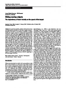
L_f_add: Left side from street number L_t_add: Left side to street number R_f_add: Right side from street number R_t_add: Right side to street number Name: street name Type: ST or AVE Zipl: Left side Zip code Zipr: Right side Zip code Speed: speed limit on this city block Oneway: a Boolean Oneway flag The following attributes are used for computing travel-time and travel-distance. Meters: length of the block in meters Drive Time: typical drive time from one end of the block to the other, in minutes This format corresponds to maps provided by the GDT Co.[6]. An intersection of two streets is the endpoint of the four block-polylines. Thus each map is an undirected graph, with the tuples representing edges of the graph. The map can be used as the underlying layer for locating moving objects (e.g. taxis). An important concept here is the trajectory of a moving object, which, intuitively, gives the route of the object along with the time at which the object will be at each point on the route. Moving Object. The route of a moving object O is specified by giving the starting address or (x,y) coordinate (start_point), the starting time and the ending address or (x,y) coordinate (end_point). An external routine available in most existing Geographic Information Systems, and which we assume is given a priori, computes the shortest cost (distance or travel-time) path in the map graph. This path denoted P(O) is given as a sequence of blocks (edges), i.e. tuples of the map. Trajectory/Route. Since P(O) is a path in the map graph, the endpoint of one block polyline is the beginning point of the next block polyline. Thus the whole route represented by P(O) is a polyline denoted L(O). For the purpose of processing spatiotemporal range queries in the language we define below, the only relevant attributes of the tuples in P(O) are Polyline and Drive-Time. Given that the trip has a starting time, for each straight line segement on L(O) we compute the time at which the object O will arrive to the point at the beginning of the segment, and the distance of the point from the start of the route. The trajectory of an object O, denoted T(O), is a relation with attributes SEQUENCE#, x, y, t, b. A tuple [i, (x,y), ti, b] in this relation indicates that (x,y) is the i'th intermediate point on O's route L(O), and O will be there at time ti. The time ti is computed based on ti-1 and the drive-time parameter for the block. In other words, the map attributes Drive Time and Polyline define an average speed for each block, and we use the length of the line segment and this average speed in order to compute each ti. Furthermore, the time at which the object is at any intermediate point on the line segment is computed by linear interpolation. In other words, a trajectory is a piece-wise linear function in 3D.

A Spatiotemporal Model and Language for Moving Objects on Road Networks

23

t

xI+1,

yI+1,

trajectory

x i , y i , tI

,

route

y x Fig. 1. A moving point representation

A trajectory may represent more than one trip of the same object. If so, the first tuple of the second trip indicates, using the Boolean attribute b, that the line segment between the endpoint of the first trip and the begin-point of the second trip is not part of any route of the object. Namely, if b is False in the i'th tuple of the trajectory, then the whereabouts of the object between ti-1 and ti are unknown. Otherwise, i.e. if b is True, then the object is "alive" between the two time points, and its location in the time interval is computed by interpolation. Next we define the type trajectory in terms of SQL DDL statements [11]: CREATE TYPE trajectory AS OBJECT (SEQUENCE# integer, x integer, y integer, t real, b boolean); The MOVING-OBJECTS relation has additional attributes such as COLOR, WEIGHT, DRIVER, etc. Then the moving objects (M_O) relation can be defined as: CREATE TYPE M_O AS OBJECT (OBJECT_id integer, T trajectory, color integer, weight integer, driver person_id); On the attribute T we use a 3D spatial index, i.e. a spatiotemporal index on 2Dspace+time [16,18]. The query for selecting the trajectory of an object O is: Q1: SELECT M_O.T FROM M_O WHERE OBJECT_id = O; Sometimes, for brevity we will use the term id, instead of OBJECT_id.

24

M. Vazirgiannis and O. Wolfson

We also need a function that returns the distance traveled along the route of an object between two points that belong to the route. Since the route of the object is defined as a polyline P, such a function is defined as: route-distance (Polyline P, 2D_point p1, 2D_point p2). There is an ordering between p1 and p2, i.e. p1 is visited before p2 along the route. Similarly we define the function route-travel-time. Both functions will be registered as a User Defined Functions (UDFs) [9] attached to the M_O type. 2.1

Definition of the Extended Functionality

The problem we address in this paper is two fold: i. the definition of a concise set of data types for moving objects and ii. the design of a small but powerful set of query predicates. The data types have been defined in the previous section. Here we will define the query predicates in terms of SQL extensions. The definition of the query predicates embedded in an SQL statement follows: SELECT LOC(id, t) | WHEN_AT(id, location-L) | FROM T WHERE id WITHIN (DISTANCE s | TRAVELTIME t) FROM R [(ALONG EXISTING PATH) | (ALONG SHORTEST PATH) ] [(ALWAYS BETWEEN) | (SOMETIMES BETWEEN) starttime AND endtime] where: - LOC(id, t) is the location on the map of a moving object identified by id, at a specific time t. The predicate returns a 2D point corresponding to the location of the object. - WHEN_AT (id, location-L) returns the time at which the moving object identified by id was at the location location-L. A set of time values is returned. The cardinality of the result is 0 if the object never passed though location-L, 1 if it passed once, and more than one if it has passed there several times. - WITHIN (DISTANCE s | TRAVELTIME t) FROM R is a predicate that requires one of the two operands: DISTANCE s or TRAVELTIME t, where s and t are real numbers. R is a point (given by its coordinates) on one of the line segments of the map, and can be obtained, for example, by geocoding an address. The predicate returns True when either: i. the object needs to travel less than s distance units in order to arrive to R or ii. the object needs to travel less than t time units in order to arrive to R. This predicate is further refined by the following two groups of quantifiers: a. ALONG EXISTING PATH and ALONG SHORTEST PATH. They are optional mutually exclusive quantifiers. The former requires the WITHIN criterion to hold along the route of the object (which implies that R belongs to the route of the object). Intuitively, this means that the object can reach R within the cost metric while traveling along its existing path. The second quantifier requires that the WITHIN criterion holds when following the shortest path between the object's current location and R. If none of them is present in the query ALONG EXISTING PATH is used as the default value. b. ALWAYS BETWEEN and SOMETIMES BETWEEN starttime AND endtime. These optional quantifiers relate to the temporal duration of the

A Spatiotemporal Model and Language for Moving Objects on Road Networks

25

WITHIN criterion. The former requires that the WITHIN criterion is true for all times between the starttime and endtime values, while the latter requires that the WITHIN criterion is true for some times between starttime and endtime. If none of them is present in the query ALWAYS BETWEEN is used as the default value, and the starttime and endtime are assigned the starttime and endtime of the trip respectively. As is evident, the WHERE clause may have regular SQL atomic conditions on regular database attributes (i.e. other than trajectory). Hereafter we elaborate on the combined semantics of the WITHIN predicate depending on the values of the route related (1. ALONG EXISTING PATH or 2. ALONG SHORTEST PATH) and time related quantifiers (A. ALWAYS BETWEEN or B. SOMETIME BETWEEN). 1A: the condition is satisfied for object if every point on o's route between starttime and endtime is within route-distance s or route-travel-time t from R (observe that using the GDT map format one can compute both travel time and distance as different cost measures). Remember, route distance (route travel time) between two points is the distance (travel time) along the current trajectory, in the forward (increasing time) direction. 2A: the condition is satisfied for an object o if every point on o's route between starttime and endtime is within travel-time t or travel-distance s from R. Here distance means distance along the shortest path. 1B: the condition is satisfied for o if some point on o's trajectory between starttime and endtime is within route-distance s or route-travel-time t from R 2B: the condition is satisfied for o if some point on o's trajectory between starttime and endtime is within distance s or travel-time t from R. Here distance means distance along the shortest path. 2.2

Spatiotemporal Index

We adopt a 3D spatiotemporal indexing scheme similar to the ones proposed in [18][10][16]. The 2D space in which the object moves, and the time dimension form a 3D space. We are interested in subsets of this domain depending on the quantifiers of the WITHIN predicate. We assume the existence of a 3D index in the database management system. Now we consider the insertion of a trajectory into the database index. To do so we enclose each 3D straight line segment into the minimum axes-parallel 3D rectangle that contains the segment. This is the Minimum Bounding Rectangle (MBR) of the trajectory segment. Observe that the trajectory segment is a diagonal of its MBR. Each line segment of a trajectory, its sequence number in the trajectory, its MBR, and the object id are inserted as a record in the 3D index. In this paper we establish the mapping of the query to a 3D query window Q, such that we retrieve all the trajectories that intersect Q. This is the only retrieval from the hard disk assuming that the contents of Q are a small part of the database and can fit into main memory. Then further processing of the query is carried out in memory. Indeed, trajectories in real-life applications like the ones we consider here contain a small number of line segments. For instance if a typical trajectory is 10km long and each city block is about 0.5 km long, then the trajectory consists of nodes.

26

M. Vazirgiannis and O. Wolfson

For Boolean combinations of spatial/temporal predicates (i.e., combination of WITHIN predicates) always the resulting set of trajectories will be the intersection (for conjunctive queries) or the union (for disjunctive ones) of the respective query spaces. Hence the spatiotemporal indexing scheme suffices for Boolean combination of queries.

3 Implementation Design of the Predicates in a Spatial Database Environment Assuming that the data types needed are implemented in an OR-DBMSs [11, 9, 4] we need to implement functions/operators that represent the functionality of these data types. These functions are implemented as user defined functions (UDFs) [4], which implement operators, or methods, that can be applied to user defined data types. In the following we review how commercial DBMSs handle the issues of definition, implementation and retrieval of user defined functions. DB2 Spatial Extender includes pre-defined functions for operations such as spatial calculations (for example, the distance between two points), comparisons (the customers located within a fivemile radius of a store), data exchange, and others. To achieve better performance, Spatial Extender functions run in an “unfenced” mode in the same address space as the database server itself. To support the Spatial Extender, IBM has also extended the notion of UDFs to allow them to be used as user-defined predicates. When a query includes, in a “where” clause, a UDF that is also defined as a predicate, the optimizer knows to look for an index on the column that would help in evaluating the predicate. User-defined predicates can be used, for example, to compare two spatial objects, such as two polygons or a point and a polygon, to see if they overlap or if one is contained within another. As predicates, UDFs trigger the use of indexes. In the case of Informix [9] user-defined routines can be written using Informix’s Stored Procedure Language (SPL), or third-generation languages such as C, C++, or Java. SPL routines contain SQL statements that are parsed, optimized, and stored in the system catalog tables in executable format, making it ideal for SQL-intensive tasks. Routines written in third-generation languages are compiled and loaded into a shared object file or dynamic link library (DLL). The routine and name of the shared object are declared to the server and once invoked, the shared object is linked to the server. Since C, C++, and Java are powerful, full-function development languages, routines written in these languages can carry out much more complicated computations than SPL functions. Commercial DBMSs provide support for alternative indexing methods in order to speed up queries involving user defined operators. In the case of IBM DB2, the DB2 index manager is open so that new index types—called index extensions—can be defined. This includes the type of index, which data types it works with, how index entries are generated from column values, and how the index can be exploited to evaluate queries efficiently. All of these index extensions are implemented through SQL extensions; this high-level API makes it relatively easy for the developer to integrate complex, user- defined index functionality. Especially for spatial data these extensions were used to implement support for spatial indexes, called grids, in the Spatial Extender. In the context of Informix, developers can index new data types using existing access methods, or add new access methods of their own. Two access methods are supported: B-tree index and R-tree index. A B-tree index organizes index information

A Spatiotemporal Model and Language for Moving Objects on Road Networks

27

and is arranged as a hierarchy of pages. The Universal Data Option introduces the Rtree index, optimized for multidimensional data. In the following we propose an implementation design of the proposed query predicates in terms of functions and operators provided by commercial DBMSs. 3.1 Query Processing Scheme for LOC and WHEN_AT Predicate LOC(id o, time t) This function gets as input an object identifier o and a time t and returns the object’s position at time t. The object o is retrieved using an index on the id attribute. If t is before the starttime (or after ending time) of the object trajectory, then the position returned is the start_point (or the end point) of the trajectory. Otherwise, we locate the two times ti, ti+1 in T(o) for which it is true that ti < t < ti+1. Then we can compute the exact position (x,y) of the object at time t by using linear interpolation: x = xi + ((xi+1- xi)/( ti+1- ti)) (ti+1-t) y = yi + ((yi+1- yi)/( ti+1- ti)) (ti+1-t) Then the 2Dpoint (x,y) is the location of the object at time t. When_at(id o, 2D_point p) The algorithm retrieves the object, and performs the following steps: a. Check if the point belongs to the route (the route of the object is obtained by disregarding the time of the Trajectory attribute) of the object. For this one can use the system provided function intersect(position, o.route). If it does not, then null is returned. b. If it belongs, then find the line segment(s) of the route to which point p belongs. c. For each one of them, compute by interpolation the time when the object was at p The object may pass more than once by the same point p so the result of the function can be a set of times. 3.2 Query Processing Scheme for WITHIN Predicate In the sequel we elaborate on the query processing scheme for the predicate WITHIN. (1At): for option 1A (ALONG EXISTING PATH/ALWAYS BETWEEN) assuming that the cost, say 5, is given in terms of travel-time: Then the query is formulated as follows: Q 2: SELECT id FROM M_O WHERE id WITHIN 5 minutes FROM R ALONG EXISTING PATH ALWAYS BETWEEN starttime and endtime /* semantics: retrieve each object for which at every time point between starttime and endtime, the object will reach R within 5 minutes, while traveling on its trajectory. */

28

M. Vazirgiannis and O. Wolfson

We use a filter and refinement approach to process this query. The filter uses the spatiotemporal index, and it is as follows. The query window Q is a line segment in 3D perpendicular to the plane t = starttime. It starts at the plane t = starttime and has length (endtime+5−starttime). Thus the line ends on the plane t = endtime+5. Using the spatiotemporal index we retrieve the set S of all the trajectories that intersect Q. These are the trajectories of objects o, that go through the point R sometime between starttime and endtime+5. The refinement step is as follows. For each trajectory T of S we consider the sub trajectory s between starttime and endtime. If the object is not "alive" on some segment of this sub-trajectory, then the trajectory is eliminated from S. Otherwise, let e1 be the time-point when T crosses R for the first time between starttime and endtime+5; let e2 be the time-point when T crosses R for the second time in the same interval; etc. Note that e1 ≥ starttime by definition. If e1 − starttime > 5, then clearly the location of the object at starttime is more than 5 minutes away from R along the trajectory, thus T is eliminated from S. Otherwise, i.e. if 5 ≥ e1 − starttime, then we consider endtime. If e1≥endtime, this means that at endtime the object has not reached the point R yet; but then clearly, from its location at endtime it will reach the point within 5 minutes, since at starttime it is not more than 5 minutes away. We conclude that the trajectory satisfies the condition, and the algorithm continues to examine the next trajectory. Otherwise, i.e. if endtime > e1, we have to examine whether the subsection of the trajectory between e1 and endtime satisfies the condition with respect to e2, e3, e4, etc. In order to verify this we assign e1 to starttime and repeat the procedure recursively. Specifically, if e2 does not exist or if e2 − starttime > 5, then clearly the location of the object at starttime is more than 5 minutes away from R along the trajectory, thus T is eliminated from S. Otherwise, i.e. if 5 ≥ e2 - starttime, then we consider endtime. If e2 ≥endtime, this means that at endtime the object has not reached the point R (for the second time) yet; but then clearly it will reach R again within 5 minutes. Thus the trajectory satisfies the condition, and the algorithm continues to examine the next trajectory. Otherwise, i.e. if endtime > e2, we have to examine whether the subsection of the trajectory between e2 and endtime satisfies the condition with respect to e3, e4, etc. The trajectories that remain in S after the refinement step constitute the answer to the query. (1Bt): for options 1B (ALONG EXISTING PATH / SOMETIME BETWEEN) assuming that the cost 5 is given in terms of travel-time: Then the query is formulated as follows. Q 3: SELECT id FROM M_O WHERE id WITHIN 5 mins FROM R ALONG EXISTING PATH SOMETIME BETWEEN starttime and endtime /* semantics: give me the objects that sometime between starttime and endtime are less than 5 minutes from R when they travel along their designated trajectory */

A Spatiotemporal Model and Language for Moving Objects on Road Networks

29

The trajectories that satisfy Q3 are the trajectories that intersect R sometime between starttime and endtime+5. This query is simpler than the 1At case. The filter step is the same, and the refinement is much simplified. Specifically, the query window Q is a line segment perpendicular to the plane t = starttime, and having length (endtime+5−starttime). Thus the line ends on the plane t = endtime+5. Using the spatiotemporal index we retrieve the set S of all the trajectories that intersect Q. These are the trajectories that cross R sometime between starttime and endtime+5. The refinement step is as follows. For each trajectory T of S we consider the trajectory segments that are "alive" between starttime and endtime. T is in the answer set if and only if at least one of them is within route-travel-time 5 minutes from R. (1As): ALONG EXISTING PATH/ ALWAYS BETWEEN) assuming that the cost 5 is given in terms of distance: The query is formulated as follows: Q 4: SELECT id FROM M_O WHERE id WITHIN 5 km FROM R ALONG EXISTING PATH ALWAYS BETWEEN starttime AND endtime We again use a filter and refinement approach to process this query. The filter uses the spatiotemporal index, and it is as follows. The query window Q is a prism having a square G as its base on the plane t = starttime, and having height (endtime − starttime). G is a square with R at its center of gravity, and with a side of length 2*5km. Using the spatiotemporal index we retrieve the set S of all the trajectories that intersect Q. All the trajectories of objects o that go through the point R in their route segment between LOC(o, starttime) and [LOC(o, endtime) plus route-distance 5km] are in S. The refinement step is as follows. For each trajectory T of S we consider the sub trajectory s between starttime and endtime. If the object is not "alive" on some segment of this sub-trajectory, then the trajectory is eliminated from S. Otherwise, let e1 be the location when T crosses R for the first time in the route segment between LOC(o,starttime) and [LOC(o,endtime) plus route-distance 5km]; let e2 be the location when T crosses R for the second time in the same interval; etc. Note that the time at e1≥ starttime by definition. If the route-distance between LOC(o,starttime) and e1 is more than 5km, then clearly the location of the object at starttime is more than 5km away from R along the trajectory, thus T is eliminated from S. Otherwise, i.e. if the route-distance between LOC(o,starttime) and e1 is not more than 5km, then we consider WHEN_AT(o,e1). If WHEN_AT(o,e1)≥endtime, this means that at endtime the object has not reached the point R yet; but then clearly, from its location at endtime the distance to R is not more than 5km, since at starttime it is not more than 5km away. We conclude that the trajectory satisfies the condition of the query, and the algorithm continues to examine the next trajectory. Otherwise, i.e. if endtime > WHEN_AT(o,e1), we have to examine whether the sub- trajectory between e1 and LOC(o,endtime) satisfies the condition with respect to e2, e3, e4, etc. In order to verify this we assign e1 to starttime and repeat the procedure recursively. Specifically, if e2 does not exist or if e2 is more than 5km away

30

M. Vazirgiannis and O. Wolfson

from LOC(o,starttime), then clearly the location of the object at starttime is more than 5km away from R along the trajectory, thus T is eliminated from S. Otherwise, i.e. if e2 is not more than 5km away from LOC(o,starttime), then we consider endtime. If endtime WHEN_AT(o,e2), we have to examine whether the sub-trajectory between e2 and endtime satisfies the condition with respect to e3, e4, etc. The trajectories that remain in S after the refinement step constitute the answer to the query. (1Bs): ALONG EXISTING PATH/ SOMETIME BETWEEN) assuming that the cost 5 is given in terms of distance: The trajectories that satisfy this predicate are the trajectories for which R is within a route-distance of 5km from some point on the sub-trajectory between LOC(o,starttime) and [LOC(o,endtime) + route-distance 5]. The query window Q is a prism having a square G as its base on the plane t = starttime, and having height (endtime - starttime). G is a square with R at its center of gravity, and with a side of length 2*5km. Using the spatiotemporal index we retrieve the set S of all the trajectories that intersect Q. All the trajectories of objects o that go through the point R in their route segment between LOC(o,starttime) and [LOC(o,endtime) + route-distance 5] are in S. The refinement step is as follows. For each trajectory T of S we consider the trajectory segments that are "alive" between starttime and endtime. T is in the answer set if and only if at least one of them is within route-distance 5km from R. (2As): ALONG SHORTEST PATH / ALWAYS BETWEEN, assuming that the cost 5 is given in terms of distance: Here we will use again the spatiotemporal index mentioned in previous sections. The query box Q must contain all the space that can be covered by an object starting from R moving along the shortest path in any direction between starttime and endtime. The query box Q will have the following dimensions: - 2D space: it will be a square centered at R having a side equal to 2*5km. (see Fig 2). - time: endtime – starttime

5km R

5km

5km

5km Fig 2. A projection of the query box Q to the x,y plane

A Spatiotemporal Model and Language for Moving Objects on Road Networks

31

It can be shown that the query box Q contains all the potential answers to the query 2As. Let us call S the set of trajectories that intersect the query box Q . We obtain S after the filter step. Consider the refinement step. First we compute the set P of whole or partial route segments that are at distance at most 5km from R. The trajectories that satisfy the predicate 2As are the trajectories of S for which the following condition is satisfied: all the trajectory segments between starttime and endtime are "alive", and their projection on the (x,y) plane is contained in P. (2Bs): ALONG SHORTEST PATH / SOMETIMES BETWEEN, assuming that the cost 5 is given in terms of distance: In this case it must be true that for at least one point in the route of the object between starttime and endtime, it is closer than 5km from R along the shortest path. Again we use the spatiotemporal index, and S as it results from the query 2As. The set P is also similarly defined. Finally, the trajectories that satisfy the predicate 2Bs are the trajectories of S for which the following condition is satisfied: some the trajectory segments between starttime and endtime are "alive", and their projection on the (x,y) plane is contained in P. (2At): ALONG SHORTEST PATH / ALWAYS BETWEEN, assuming that the cost 5 is given in terms of travel time: The filter step constructs the query Q as follows. First we compute the set M of route segments (consisting of the points) that are at travel-time at most 5 minutes from R. We do so by using the standard shortest path algorithm on the map graph. For each route segment r we construct a rectangle in 3D with base r on the plane t = starttime, and a height (endtime−starttime) perpendicular to that plane. The query Q consists of all these rectangles. Then we retrieve the set S of trajectories that intersect this set of rectangles. The refinement step is as follows. For each trajectory T in S we compute the set T.M of route segments that the object travels between starttime and endtime. If the object is not alive on all these route segments, then T is eliminated from S. The trajectories that satisfy the query are: the subset of S consisting of each trajectory T for which T.M is a subset of M. (2Bt): ALONG SHORTEST PATH / SOMETIME BETWEEN, assuming that the cost 5 is given in terms of travel time: The filter step is the same as in 2At. The refinement step is as follows. For each trajectory T in S we compute the set T.M of route segments that the object travels between starttime and endtime, and on which the object is "alive". The trajectories that satisfy the query are: the subset of S consisting of each trajectory T for which the intersection of T.M and M is nonempty.

4 Related Work Temporal data models provide built-in support for capturing one or more temporal aspects of the database entities. It is conceptually straightforward to also associate the database entities with spatial values. Concrete proposals include a variant of Gadia's temporal model [14, Ch. 2], a derivative of this model [2], and STSQL [1].

32

M. Vazirgiannis and O. Wolfson

Essentially, these proposals introduce functions from the product of time and space to base domains, and they provide languages for querying the resulting databases. These proposals are orthogonal to the specifics of types and simply abstractly assume types of arbitrary subsets of space and time; no frameworks of spatiotemporal types are defined. The data model by Worboys [17] represents this approach. Here, spatial objects are associated with two temporal aspects, and a set of operators for querying is provided. However, this model does not provide an expressive type system, but basically proposes only a single type, termed ST-complex, with a limited set of operations. In addition, two papers exist that consider spatiotemporal data as a sequence of spatial snapshots and in this context address implementation issues related to the representation of discrete changes of spatial regions over time [12]. Reference [13] presents a model for moving objects along with a query language. However, the new language constructs there are purely temporal and nonstandard, and the model does not capture full trajectories. In contrast, the constructs in this paper are refinements of standard spatiotemporal range queries. Work in constraint databases is applicable to spatiotemporal settings, as arbitrary shapes in multidimensional spaces can be described. Papers that explicitly address spatiotemporal examples and models include [7, 3]. However, this kind of work essentially assumes the single type "set of constraints," and is not concerned with types in the traditional sense. Operations for querying are basically those of relational algebra on infinite point sets. Recent work recognizes the need to include other operations, e.g., distance [7]. The Informix Dynamic Server with Universal Data Option covers type extensibility [8]. So-called DataBlade modules may be used with the system, thus covering new types and associated functions that may be used in columns of database tables. Of relevance to this paper, the Informix Geodetic DataBlade Module [8] covers types for time instants and intervals as well as spatial types for points, line segments, strings, rings, polygons, boxes, circles, ellipses, and coordinate pairs. Informix does not cover any integrated spatiotemporal data types. Limited spatiotemporal data support may be obtained only by associating separate time and spatial values. The framework put forward in this paper provides a foundation allowing Informix or a third-party developer to develop a DataBlade that extends Informix with expressive and truly spatiotemporal data types. Since 1996, the Oracle DBMS has offered a so-called spatial data option, also termed a Spatial Cartridge, that allows the user to better manage spatial data [11]. Current support encompasses geometric forms such as points and point clusters, lines and line strings, and polygons and complex polygons with holes. However, no spatiotemporal types are available in Oracle. The support offered by Oracle resembles the support offered by DB2's Spatial Extender [4], which offers spatial types such as point, line, and polygon, along with \multi-" versions of these, as well as associated functions, yielding several spatial ADT's. Like Oracle, spatiotemporal types are absent. A recent effort for a foundation of spatiotemporal data types and query language design appears in [5], where all the design is based on the moving point and moving region data types and the associated operations. One of the most recent efforts dealing with indexing of moving points is [10]. There the authors deal mainly with the problem of moving objects on a line and they propose a dual representation that is claimed to give logarithmic response time to range queries. That paper only covers indexing issues (not modeling or linguistic issues as we do here), and considers standard range queries.

A Spatiotemporal Model and Language for Moving Objects on Road Networks

33

In [18] the authors propose a comprehensive approach to embedding moving objects support in a commercial DBMS. Several issues are addressed such as: indexing moving objects, uncertainty regarding the position of an object, dynamic behavior evolving with time. However, the model and language constructs in this paper are new.

5 Conclusions In this paper we introduced a model for moving objects on road networks. The road network is represented by an electronic map. The connection between the moving object trajectory model and the road network represents one of the innovative aspects of this work. We also defined a small set of expressive predicates that can effectively be implemented in terms of existing spatial operators within commercial database/GIS systems. The language we propose handles a large number of reasonable queries about moving objects. Although the model paradigm was build on GDT maps as a running example, the design of the predicates is applicable to other contexts in which objects move in a spatial grid. The design presented in the paper is directly applicable to such contexts, provided that the appropriate spatial grid model and associated support functions (such as the one for shortest path or distance computation) are provided. Another issue that arises is the representation of non polygonal trajectories. This case will be further investigated. As a first approach it can be treated in two ways: - either approximated by polygonal lines using interpolation and or extrapolation techniques - or represented by mathematical expressions – patterns- that represent trajectories in as a continuous function of time. Further work will be committed in the following directions: Deal with uncertainty features. This work will be based on initial work on spatial relationships [15]. - Consider the dual model as the database representations scheme. - Implementation of the predicates defined in the paper, and performance evaluation. We plan to have two parallel implementations based on different database products exploiting their respective type extension facilities. -

Acknowledgement. We wish to thank Goce Trajcevski for helpful discussions

References [1] [2] [3]

M. H. Boehlen, C. S. Jensen, and B. Skjellaug.: Spatiotemporal Database Support for Legacy Applications. In proceedings of ACM Symposium on Applied Computing, 1998. 226-234. T. S. Cheng and S. K. Gadia.: A Pattern Matching Language for Spatiotemporal Databases. In Proceedings of the ACM Conference on Information and Knowledge Management (1994) 288-295. J. Chomicki and P. Revesz.: Constraint-Based Interoperability of Spatiotemporal Dataases. In proceedings of the 5th International Symposium on Large Spatial Databases (1997) 142-161.

34 [4] [5]

[6] [7] [8] [9] [10] [11] [12] [13] [14] [15] [16] [17] [18]

M. Vazirgiannis and O. Wolfson J. R. Davis. IBM's DB2 Spatial Extender: Managing Geo-Spatial Information Within The DBMS. Technical report, IBM Corporation, May 1998. Ralf Hartmut Güting, Michael H. Böhlen, Martin Erwig, Christian S. Jensen, Nikos A. Lorentzos, Markus Schneider, and Michalis Vazirgiannis.: A Foundation for Representing and Querying Moving Objects, in ACM-Transactions on Database Systems journal (2000), 25(1). 1-42. Geographic Data Technology Co. http://www.geographic.com/index.cfm, 2000. S. Grumbach, P. Rigaux, and L. Segoufin: The Dedale System for Complex Spatial Queries: In Proceedings of the ACM SIGMOD International Conference on Management of Data (1998) 213-224 Extending Informix Universal Server: Data Types. Informix Press, March 1997. Informix DataBlade Technology: Transforming Data into Smart Data, 1999 G. Kollios, D. Gunopoulos, V. Tsotras: On indexing mobile objects. In the proceedings of ACM PODS (1999) Oracle8: Spatial Cartridge, An Oracle Technical White Paper, Oracle Corporation, June 1997. H. Raafat, Z. Yang, and D. Gauthier: Relational Spatial Topologies for Historical Geographic Information. International Journal of Geographical Information Systems (1993) 8(2) 163-173 A. P. Sistla, O. Wolfson, S. Chamberlain, and S. Dao: Modeling and Querying Moving Objects. In proceedings of the International Conference on Data Engineering (1997) 422432 A. Tansel, J. Clifford, S. Gadia, S. Jajodia, A. Segev, and R. T. Snodgrass: Temporal Databases: Theory, Design, and Implementation, Benjamin/Cummings Publishing Company, Inc., Redwood City, California, 1993. M. Vazirgiannis: Uncertainty handling in spatial relationships. In proceedings of ACMSAC conference (2000). M. Vazirgiannis, Y. Theodoridis, T. Sellis: Spatiotemporal Composition and Indexing for Large Multimedia Applications. In ACM/Springer-Verlag Multimedia Systems Journal. 6(4), 1998. 284-298. F. Worboys: A unified model for spatial and temporal information. The Computer Journal, 37(1). 25-34. O. Wolfson, B. Xu, S. Chamberlain, L. Jiang: Moving Objects DataBases: Issues and solutions. In proceedings of SSDB conference 1998. 111-122.

Appendix A. Primitives Provided by Commercial Products In this section we refer to the spatial and other functions provided by commercial products and are exploited in our design. The primitives indicates by * are provided by both Informix Spatial Datablade and ArcView. The ones without * are provided only by ArcView. Function name *contains(shape1,shape2) *intersect(shape1,shape2) along(polyline,dist) selectby(shape) traveltime(polyline p).

Semantics returns TRUE if shape1 contains shape2 returns TRUE shape1 intersect shape2 returns a point on a polyline, the route distance of which is "dist" length units away. selects the features that intersect “shape” returns the travel time along the polyline p in time units

A Spatiotemporal Model and Language for Moving Objects on Road Networks

35

Although Arcview/Informix do not use the notion of time, they use the notion of cost. So given GDT maps, cost can be interpreted as travel-time or distance. IBM Spatial Extender [4] provides the following functions for spatial data manipulation: Comparison functions: contains, cross, disjoint, equals, intersects, overlap, touch, within, envelopes intersect Relationship functions: common point, embedded point, line cross, area intersect, interior intersect, etc. Combination functions: difference, symmetric difference, intersection, overlay, union, etc. Calculation functions: area, boundary, centroid, distance, endpoint, length, minimum distance, etc. Data-exchange functions: astext (for Open GIS well-known text representation), asbinary (for Open GIS well-known binary representation), asbinaryshape (for ESRI shape representation), etc. Transformation functions: buffer, locatealong, locatebetween, convexhull, etc.