to determine the most important performance variables to test, and ..... server. Pixel noise is a critical limiting factor in CT since much soft tissue detail is low ...
AAPM REPORT NO. 39
SPECIFICATION AND ACCEPTANCE TESTING OF COMPUTED TOMOGRAPHY SCANNERS
i
Published for the American Association of Physicists in Medicine by the American Institute of Physics
AAPM REPORT NO. 39
SPECIFICATION AND ACCEPTANCE TESTING OF COMPUTED TOMOGRAPHY SCANNERS Report of Task Group 2 Diagnostic X-Ray Imaging Committee AAPM Members Pei-Jan Paul Lin (Task Group Co-Chairman) Thomas J. Beck (Task Group Co-Chairman) Caridad Borras Gerald Cohen Robert A. Jucius Robert J. Kriz Edward L. Nickoloff Lawrence N. Rothenberg Keith J. Strauss Theodore Villafana Additional Contributors Robert K. Cacak Joel E. Gray Thomas N. Hangartner R. Edward Hendrick Raymond P. Rossi May 1993 Published for the American Association of Physicists in Medicine by the American Institute of Physics
DISCLAIMER: This publication is based on sources and information believed to be reliable, but the AAPM and the editors disclaim any warranty or liability based on or relating to the contents of this publication. The AAPM does not endorse any products, manufacturers or suppliers. Nothing in this publication should be interpreted as implying such endorsement. Further copies of this report may be obtained from: American Association of Physicists in Medicine 335 East 45th Street New York, NY 10017
International Standard Book Number: 1-56396-230-6 International Standard Serial Number: 0271-7344 ©1993 by the American Association of Physicists in Medicine
All rights reserved. No part of this publication may be reproduced, stored in a retrieval system, or transmitted in any form or by any means (electronic, mechanical, photocopying, recording, or otherwise) without the prior written permission of the publisher.
Published by the American Institute of Physics, Inc. 335 East 45th Street, New York, NY 10017
Printed in the United States of America
Preface The Computed Tomography (CT) Scanner Task Group was formed to provide a reference document of suggested procedures for acceptance testing of CT systems for clinical medical physicists. The AAPM first addressed performance testing of CT systems with the publication of AAPM Report No. 1, “Phantoms for Performance Evaluation and Quality Assurance of CT Scanners”. Since publication of Report No. 1 in 1977, CT system designs have evolved and research has improved our understanding of principles and limitations of CT systems. These changes in technology and our understanding of them prompted the formation of this task group. This report is intended to be a source of acceptance testing procedures, as well as an educational tool for those medical physicists whose primary responsibilities lie in areas other than diagnostic imaging. In addition to acceptance testing procedures, the related issues of specification writing and radiation shielding design are also discussed.
Preface . . . . . . . . . . . . . . . . . . . . . . . . . . . . . . . . . . . . . . . . . . . . . . . . . . . .iii I.Introduction.................................................................1 A. THE BID REQUEST . . . . . . . . . . . . . . . . . . ........................... . . . . . . . . . . . . . . . . . . . . . . . . . . . . . . .2 B. EVALUATING NEEDS OF THE USER........................................................................................2 C. EQUIPMENT SELECTION...............................................................................................................3 D. SPECIFICATION WRITING ..................... . . . . . . . . . . . . . . . . . . . . . . . . . . . . . . . . . . . . . . . . . . . 3 II. Shielding Design........................................................................................4 III. Performance Evaluation. . . . . . . . . . . . . . . . . . . . . . . . . . . . . . . . . . . . . . . . . . . . . . . . . . . .9 A. PERFORMANCE OF ELECTROMECHANICAL COMPONENTS ....................... . . . . . . . . . . . . . . .13 1. Scan Localization Light Accuracy ............................. ..14 2. Alignment of Table to Gantry . . . . . . . . . . . . . . . . . . . . . . . . . . . . . . . . . . . . . . 15 3. Table/Gantry Tilt .................. . . . . . . . . . . . . .15 4. Slice Localization From Radiographic (Scout) Image . . . . . . .17 5. Table Incrementation . . . . . . . . . . . . . . . . . . . . . . . . . . . . . . . . . . . . . . . . . . . . . . . ...18 6. Collimation . . . . . . . . . . . . . . . . . . . . . . . . . . . . . . . . . . . . . . . . . . . . . . . . . . . . . . . . . . . . . 19 a. Radiation Profile Width . . . . . . . . . . . . . . . . . . . . . . . . . . . . . . . . . . . . . . . . 19 b. Sensitivity Profile Width................................................................20 7. The X-ray Generator..............................................................23 B. IMAGE QUALITY.......................................................................................26 1. Random Uncertainties in Pixel Value...........................................26 2 . Systematic Uncertainties in Pixel Value . . . . . . . . . . . . . . . . . . . . . . ..3 1 a. Image Artifacts . . . . . . . . . . . . . . . . . . .34 1) Geometric Artifacts.......................................................34 a) Aliasing.................................................................34 b) Edge Gradient Streaks .............................................34 c) Geometric Misalignment....................................................35 d) Motion Artifacts......................................................35 2) Reconstruction Algorithm Effects ..........................................35 a) Point Spread Effect..................................................35 b) Edge Enhancement Artifacts . . . . . . . . . . . . . . . . . . . . . . 35 3) Attenuation Measurement Errors . . . . . . . . . . . . . . . . . . . . . . 36 a) Detector or Source Variations . . . . . . . . . . . . . . . . . . . . 36 b) Nonlinear Attenuation Errors . . . . . . . . . . . . . . . . . . . . . 36 b. Measurement of Systematic Pixel Error . . . . . . . . . . . . . . . . . . . 37 1) Field Uniformity........................................................ 37 2) Considerations in Quantitative CT................................ .........39 3. Spatial Frequency Limits...........................................................41 a. High Contrast Spatial Frequency Limits . . . . . . . . . . . . . . . . . .41 1) Measuring Resolution With A Resolution Pattern . . . . . . . . . . . . . . . . . . . . . . . . . . . . . . . . . . . . . 43 2) Modulation Transfer Function Measurement.......44
b. Low Contrast Spatial Frequency Limits . . . . . . . . . . . . . . . . . . . 47 Video Display and Multiformat Camera Image Quality.....49 a. Visual Display Screen Setup and Quality Control......50 b. Setup of Multiformat Camera Image . . . . . . . . . . . . . . . . . . . . . . . 51 C. Radiation Dose . . . . . . . . . . . . . . . . . . . . . . . . . . . . . . . . . . . . . . . . . . . . . . . . . . . . . . . . . . . . . . . 52 1. Ion Chamber Dosimetry . . . . . . . . . . . . . . . . . ...........................54 2. TLD Dosimetry . . . . . . . . . . . . . . . . . . . . . . . . . . . . . . . . . .. . . . . . . . . . . . . . . 56 I V . S u m m a r y . . . . . . . . .................................................................57 REFERENCES . . . . . . . . . . . . . . .......................................................... 5 9 Appendix A: SPECIFIC TECHNICAL AND PERFORMANCE INFORMATION FOR C T SCANNER BID SUBMISSION . . . . . . . . . . 63 Appendix B: PHANTOMS FOR ACCEPTANCE TESTING OF X-RAY TRANSMISSION CT SCANNING SYSTEMS . . . . . . . . . . . . . . 88 4.
I. Introduction The medical physicist can perform a critical role throughout the selection, purchase and acceptance of any complex expensive medical imaging system, such as an x-ray computed tomography (CT) scanner. Early involvement in the writing of the bid request can ensure that the appropriate technical data are supplied by the vendors in a format permitting a reasonable comparison. The expertise of the medical physicist can be used to analyze these specifications so that the nontechnical user can make an informed decision about which equipment best matches the clinical needs. Once the purchase decision is made, the physicist should be involved in site preparation and shielding design to ensure that radiation protection requirements are met and appropriate reports are submitted to regulatory authorities. Prior to acceptance of the system by the user, the physicist should make a thorough evaluation of the system performance and radiation characteristics to be certain that the system meets the specifications of the manufacturer and any additional requirements spelled out in the purchase document. Finally, the medical physicist can employ acceptance test data for x-ray machine inspection/registration reports required by some regulatory authorities. The primary concerns of clinical medical physicists in diagnostic radiology are image quality, radiation dose, and radiation protection. This document, therefore, is concentrated on scanner characteristics which directly or indirectly influence one of these concerns. Emphasis is placed on performance characteristics that can be quantified by a medical physicist using widely available instruments and apparatus. Testing methods described in this document are suggestions and should not be interpreted as the only acceptable methods. Some procedures may require modification to address unique design features of a given scanner. The experienced physicist will find that different tests can be combined to make best use of limited scanner access time. The acceptance test is a series of measurements performed by the physicist to verify that a CT system conforms to vendor technical specifications or to specifications mutually agreed upon by buyer and vendor. Often, a proviso for acceptance testing is written into the bid request which indicates who will do the testing, what tests will be performed, and what level of performance is acceptable to the buyer.
1
A. THE BID REQUEST The bid request is a document submitted by the purchaser to potential CT system vendors which lists, in generic terms, system capabilities desired by the purchaser and any special business terms or conditions required. The physicist should ensure that sufficient technical detail is requested to allow a comparison of performance specifications. In this regard, a typical bid request should solicit the following:
•
A full set of technical specifications detailing system performance in terms of spatial resolution, image noise and radiation dose for all standard scan settings.
•
A set of typical multiformat images annotated with scan parameters used, and showing anatomy of clinical interest to the purchaser.
•
A list of local purchasers to facilitate site visits.
•
Typical architectural layouts indicating space, weight, electrical, and thermal requirements.
•
Typical radiation exposure levels around the CT gantry for shielding design.
•
Details of warranties, service contracts, and projected costs of contract and non-contract service over the first three years after warranty expiration.
Comparison of technical specifications can be difficult when supplied in dissimilar formats. In the interest of uniformity, a sample bid questionnaire is included as Appendix A. B. EVALUATING NEEDS OF THE USER Specific clinical needs to be determined include: patient load, type of patients examined (e.g., ambulatory, inpatient, adult, pediatric) and principal kinds of examinations anticipated. This provides insight into throughput, image archiving requirements and shielding design, and has an impact on system cost. More expensive systems may have more detectors, more pow2
erful computers, more flexible software, faster scan and reconstruction times, and better spatial resolution. Options such as separate diagnostic consoles, multiformat cameras, fast-cycle reconstructions, image archiving devices and special purpose software can add significantly to the total price. A careful technical evaluation can provide maximum value to the purchaser by matching the system configuration to actual needs. C. EQUIPMENT SELECTION After bids are received, technical differences between them can be simplified by tabulating technical specifications of each scanner for a “side-by-side” comparison. This should be accompanied by a non-technical commentary which relates relative importance of specifications to the user’s specific needs. “Trade-offs” of performance levels should be pointed out, i.e., the dose and spatial resolution at optimal settings for low contrast discrimination, the dose and noise level at optimal spatial resolution settings, etc. Prior to the final purchase decision, a site visit may be appropriate, particularly if new or unfamiliar systems arc considered. If a system employs significantly new technology, a few selected performance measurements by the physicist can prove useful. Because CT systems are inherently complex and prone to failure, the availability and quality of service should weigh heavily in the purchase decision. Since service quality varies from one locale to the next, it is wise to confer with other local users prior to purchase. Warranties should be carefully reviewed and compared with regard to duration and components covered. Twelve-month warranties are typical for hardware and may or may not include x-ray tubes. Service contracts are commonly priced as a percentage of total system price (typically 8 to 12%). D. SPECIFICATION WRITING Once the purchase decision is made, the buyer may request that the physicist write performance specifications into the purchase agreement In some institutions, specifications are sent to vendors with the bid request. In any case, the following should be kept in mind: Specify only parameters with a measurably impact on some aspect of performance.
3
•
Ensure that specifications are within the performance capability of the CT system in question.
•
Be certain that a reliable, acceptable means of measurement is available for each specification.
•
Either describe measurement methods or reference standard techniques to allow the manufacturer to know how a given parameter is to be tested.
Specifications may also address system reliability by requesting a guaranteed “up-time” of 95% for the warranty period. The proviso may also include penalties for excessive down-time, such as one month of warranty extension for each 1% of down-time beyond the specified 5% (see Appendix A).
II. Shielding Design Like any radiation emitting system, consideration must be given to protection of personnel and others in the immediate vicinity of the CT system. Unfortunately, the characteristics of a CT system do not readily lend themselves to the standard shielding design methods of NCRP Report No. 491. Two methods will be described: direct use of isoexposure contours, and an isotropic point source method adapted to that of NCRP Report No. 49. Manufacturers can provide measured exposure levels in the gantry vicinity under average scan conditions, typically in the form of isoexposure contours, (see Figure 1). Isoexposure curves show measurements of exposure per scan in air while scanning a cylindrical phantom. Measured values typically represent scatter from the portion of the phantom within the scan field and do not suggest significant contributions from leakage or transmitted primary radiation. All barriers may be reasonably treated as secondary barriers. Isoexposure contours may be used directly in shielding design, in which case two drawings are necessary, one in the horizontal plane (floor plan) and one in the vertical plane (elevation plan) scaled to the architectural plan. Exposure contour drawings can be superimposed on the architectural plan, and exposure levels either read directly or extrapolated (inverse square) to occupied areas, Exposure per scan values are then scaled to the total weekly workload of the scanner. A linear correction should be used, if slice width is different from that under which exposure contours were measured.
4
Figure 1: Typical isoexposure contours around CT gantry during scanning. Units are arbitrary, depending on scanner and scan conditions. (Generally available from scanner manufacturer).
An alternative shielding design method adapted from the standard methodology of NCRP No. 49 is described as follows:
5
For simplicity, secondary radiation is assumed to be isotropically emanating from the center of the gantry axis (the gantry isocenter). This ignores inherent shielding in the “shadow” of the gantry, hence is conservative in certain directions. The assumed exposure rate (X,) is the “worst case” measured value at one meter from the gantry isocenter in mGy/mA-min (air kerma), for the largest slice width on a body size phantom. As shown in Figure 1, the worst case exposure rate is at an angle of roughly 45° to the gantry axis. Some typical values of Xs normalized to one meter for both body and head scans are listed in Table 1. The required barrier transmission (B), at any location to be shielded, can then be obtained from the expression 1:
Workload can be calculated in mA-minutes/week as:
Workloads for 120-130 kV machines may range from 5,000 to as high as 20,000 mA-min/week for heavily used systems, As in most shielding circumstances it is wise to be reasonably conservative, overestimating workloads to allow for changes in technique or patient load. Given the barrier transmission (B) the required shielding thickness of a specific material can be computed from the formalism of Archer et a1. 2:
6
where t is the required barrier thickness (in mm for lead, cm for all other materials) of specific shielding material. B is the barrier transmission, while a, b, and g are fitting constants from Simpkin 3 . The coefficients appropriate for CT energies and beam qualities for a number of common structural and shielding materials are reproduced in Table 2. Use of these coefficients is illustrated in the following example:
A control area is 2.5 m from the gantry isocenter for a system where heavy use is anticipated at a tube potential of 140 kVp. Assuming a workload of 20,000 mA-min/wk, a (conservative) design air kerma of 0.1 mGy/wk, an occupancy factor of 1 and X s (Table 1, GE 9800B, 42 cm phantom) of 3.8 • 10-3 mGy/mA-min @ 1 m, the barrier transmission from Equation [1] is then:
The coefficients for lead at 140 kVp from Table 2 are entered into Equation [3] as follows:
Similarly, using the fitting coefficients from Table 2 for concrete, gypsum board, steel and plate glass results in required thicknesses of 10 cm, 27.0 cm, 1.01 cm and 12 cm, respectively. In practice, the method is considerably simplified by incorporating the mathematics of Equation [3] and the coefficients of Table 2 into a simple computer program or spreadsheet.
7
Table 1:
Normalized scatter air kerma rates (Xs) in mGy/mA-min measured at 1 m for selected CT scanners, and conditions as indicated.
8
Table 2:
Shielding coefficients for computing thickness of shielding material required for Equation [3]. Coefficients yield thickness (t) in cm for all materials except lead, where t is in mm.
III. Performance Evaluation Performance of any scanner varies with operating conditions, and most systems provide more combinations than can be practically tested. Nevertheless, the acceptance test must acquire sufficient data to adequately characterize the system’s performance. Before beginning, consider the following:
•
Review clinical needs, scanner specifications and design principles to determine the most important performance variables to test, and include only those that could affect an important performance measurement.
•
Devise a short list of 4-5 “standard” scanning conditions, either suggested by the manufacturer or by local users. Typically this would include: standard body, standard head, spine, pediatric body and pediatric head, as appropriate to the installation. All pertinent performance tests should be done under each standard condition to provide a performance baseline for comparison.
•
Determine a few more scanning conditions that test performance limits, i.e., the fastest scan, the highest resolution scan, the lowest noise scan, etc., and relate results to baseline conditions.
9
Table 3:
CT image quality and electromechanical acceptance tests.
•
Determine both benefits and trade-offs of a given protocol, e.g., in the highest resolution scan determine the consequences in image noise, dose, presence of artifacts, etc.
Performance may also be influenced by the properties of the computer system, and by major electromechanical components, i.e., x-ray generator, xray tube, collimators, alignment lights, patient table, etc. Computer systems are evolving too rapidly for inclusion, but consideration of image quality is preceded by a discussion of direct and indirect performance measures of major electromechanical components. It is suggested that electromechanical tests precede those for image quality. Major discrepancies may influence image quality or dose and should be corrected prior to proceeding with other tests. An overview of the principal tests, their alternatives and priority are listed in Table 3, together with pertinent comments. For convenience, a listing of tools required for all tests is listed in Table 4. Scanner performance and the interpretation of certain tests are influenced somewhat by scanner design. For the purposes of this document the following conventions are used (most but not all system configurations will fall into one of the following categories): Second Generation Scanner: A mostly outmoded design with multiple detectors which operates in a translational motion during image acquisition, with rotation between projections. Generally employs a stationary anode x-ray tube and a constant potential x-ray generator. Third Generation Scanner: The most common system design which uses a x-ray tube collimated to a fan beam directed at an arc-shaped array of detectors on the opposite side of the patient. Both x-ray tube and detector array rotate during image acquisition. Generally employs a rotating anode x-ray tube, and the generator may or may not be pulsed. Xenon gas detectors are only used with third generation designs. May employ slip rings to permit continuous rotation for spiral scanning. Some less expensive versions employ an asymmetric fan beam coupled to a detector array which samples half of the gantry aperture. Fourth Generation Scanner: A scanner design which incorporates a ring of stationary detectors in which the x-ray tube rotates in a concentric path inside the detector ring. Generally employs a rotating anode x-ray tube and a constant potential generator. May employ slip rings to permit continuous rotation for spiral scanning. A variation on this design uses a nutating
11
motion of the detector ring so that the x-ray tube can be placed outside the detector ring. In this configuration, the detector ring tilts back away from the position of the x-ray tube as it rotates (so the beam doesn’t intercept the outer ring). Opposite the position of the x-ray tube the detector ring tilts forward to intercept the beam transmitted through the patient.
Table 4: Equipment required for CT acceptance tests.
12
A. PERFORMANCE OF ELECTROMECHANICAL COMPONENTS CT scanners incorporate specialized x-ray generators and a number of electromechanical components designed to localize and define the scan plane to the patient’s anatomy. This category includes gantry and patient table motions, scan alignment lights and x-ray beam collimators. Since the x-ray generator and electromechanical components are subject to miscalibration, mechanical misalignment or other problems, careful testing is required.
13
1. Scan Localization Light Accuracy Purpose: To test congruence of scan localization light and scan plane. Patient anatomy to be scanned is often defined by scan alignment lights. Alignment lights may be located within the gantry at the slice plane, outside the gantry at a reference distance from the scan plane, or both. If both internal and external alignment lights are supplied, and are independently aligned, both should be tested. Tools needed: Sheet of therapy localization film, film backing plate, adhesive tape and sharp pin or needle. Method:
•
Tape film to backing plate with film edges aligned parallel to plate edges. Tape plate in position oriented vertically along long axis of table and raise table to head scan position. If both internal and external alignment lights are provided, position plate so that both lights are visible on film surface (if possible).
•
Turn on internal alignment light and mark light location on film by piercing film pack with pin at several points along middle of illuminated line. Repeat for external light, but put unique pattern of pin pricks near each illuminated line for later identification.
•
Expose film at inner light location using narrowest slice setting at ~50-100 mAs, 120-140 kVp. For external light, increment table to light position under software control and repeat scan.
•
For time savings, combine this test using same film for Gantry/table Tilt test (Section III.A.3); use same setup but fresh film for Radiation Profile (Section III.A.6.a).
Interpretation: Measure alignment error from holes in processed film to midpoint of radiation field. In absence of manufacturer’s specifications, error should not exceed ±2.0 mm. Accuracy of external light systems depends on both table incrementation accuracy and light alignment, since they are designed to indicate a plane a specific distance from the scan plane.
14
2. Alignment of Table to Gantry Purpose: To ensure that long axis of table is horizontally aligned with a vertical line through the scanner rotational axis. Rationale: Misalignment can cause image artifacts with large patients if patient extends out of the sampled area. Tools needed: Tape measure and adhesive tape. Optional - a plumb bob (string with a pointed weight on the end). Method:
•
Place piece of tape on middle of tabletop, locate table midline with ruler and mark on tape.
•
With table and gantry untilted, extend tabletop into gantry to tape mark.
•
Locate vertical midline of gantry opening with tape measure across largest horizontal diameter or alternatively hang plumb bob from top midpoint of gantry opening. Mark gantry midline on adhesive tape on tabletop.
Interpretation: Measure horizontal inaccuracy from marks on adhesive tape. In absence of manufacturer’s specifications, gantry midline should be within ±5 mm of table midline. 3. Table/Gantry Tilt Purpose: To determine accuracy of tilt indicators and to ensure that specified tilt can be accomplished under clinical conditions. (See alternative Slice Localization From Radiographic (Scout) Image test). Rationale: Tilt indicators on gantry or table may not correspond to actual tilt or to that indicated on computer display. Some scanners may collide with the patient at extremes of tilt under some clinical conditions. Most scanners accomplish nonorthogonal scan planes by tilting the gantry, but some angle the table. Most table-tilting systems angle the table relative to the horizontal plane; however, pivoting of the table relative to the vertical plane is also seen.
15
Tools needed: Carpenter’s spirit level, protractor, adhesive tape, sheet of therapy localization film, film backing plate, and tape measure with millimeter ruling.
Tape film centered to side of acrylic plate, with film edge carefully aligned to edge of plate. Lower table to body scan position. For systems which tilt the gantry or table in vertical plane: Align plate with long axis of table, parallel to vertical plane (verify with spirit level). Fix in position with tape extending from table edge to table edge across top of plate. For tables tilting in horizontal plane: Place plate flat on tabletop with plate edge aligned to table long axis; tape into position. Move tabletop into gantry opening: center plate to alignment light. Expose the film at inner light location using narrowest slice setting at ~ 50-100 mAs, 120-140 kVp. Tilt gantry (table) to one extreme from operators console: record angle indicated on gantry (table) and operators console, repeat exposure. Measure gantry clearance from closest point on gantry to table midline. Tilt to opposite extreme, record indicated angles, repeat exposure and clearance measurement. Interpretation: Measure tilt angles between density lines on processed film using protractor; express angles relative to density line from untilted position. In absence of manufacturer’s specifications, tilt inaccuracies should be less than 3°; consoIe and gantry angle indicators, however, should agree exactly. Ideally, gantry clearance at the extremes of tilt should permit the scanning of at least a 30 cm patient.
16
4. Slice Localization From Radiographic (Scout) Image Purpose: To determine correspondence of localization image parameters with actual slice position and angle (see alternative Table Gantry Tilt test). Rationale: Errors can be problematic in quantitative CT work in the spine. Using an initial localization image of the patient, the measurement slice must be accurately positioned in the center of the vertebral body at an angle parallel to the end-plates. Errors in axial position or angle can cause inclusion of the dense end-plates in the slice intended to measure only trabecular bone in the center region. Tools needed: Test object with two 45° wire cross-hairs (see Figure B-3, Appendix B) and protractor. Method:
•
Incline test object disk at an angle to be tested (verify with protractor) and position it on the scanner table such that the wire crosshairs are visible in a lateral view. Take lateral localization radiograph. Under computer control define slice position and slice angle to pass through intersections of the two cross-hairs.
•
Scan phantom with narrowest slice and highest resolution settings. The correctly positioned image should show two dense objects in a vertical orientation, corresponding to intersections of the two sets of wires.
•
If one or both cross hairs show the wires vertically separated from each other, repeat scan at one mm spacing and same tilt angle on either side of the first slice. This will permit determination of the displacement and angle error.
•
Repeat procedure for an arbitrary inclination angle in the opposite direction.
Interpretation: Because the two wires in each cross-hair are. 45° apart and one wire is roughly perpendicular to the scan plane, the distance between the two in the image gives the table position error. Combining the position errors of both cross-hairs provides the gantry angulation error. This test
17
should be repeated periodically since indicators for table axial position, height and tilt can change over time. 5. Table Incrementation Purpose: To determine accuracy and reproducibility of longitudinal table motion. Rationale: Under computer control from operators console the patient table must be able to accurately and reproducibly move the patient to any indicated position in the scan field. Accuracy is critical since it determines relative locations of image sections and influences the multi-scan dose. Tools needed: 10-30 cm ruler with mm ruling, bent paper clip for a pointer and adhesive tape. Method:
•
Tape ruler along tabletop edge, near foot end. Tape pointer (end of paper clip) on table frame opposite midpoint of ruler with pointer directed at ruler midpoint. Zero table position.
•
Load table with 70-80 kg (150-180 lb), c.g., have assistant lie on table.
•
From control console, note indicated table position. Under computer control move tabletop 300-500 mm in one direction, and back to original position.
•
Record relative distance from starting position (if any) indicated by pointer and ruler.
•
Repeat measurement twice more with same direction of table motion, then three times in opposite direction.
Interpretation: In the absence of specifications, both the standard deviation and the average error should be less than 3 mm, Note whether error is systematic (in one direction) or random.
18
6. Collimation A CT scan samples a thin slab of tissue; ideally only the imaged slab is irradiated, and its thickness equals the selected slice width. Inaccuracies arise from scanner &sign limitations and calibration of collimator settings. Most systems collimate the z axis dimension of the x-ray beam at both the source (patient collimation) and detectors (postpatient collimation). Width of the imaged slice (from sensitivity profile) is determined by both sets of collimators. Width of the tissue irradiated (from radiation profile) is a function only of the prepatient collimator. Measurements of radiation and sensitivity profiles are best interpreted together. a. Radiation Profile Width Purpose: To determine accuracy of prepatient collimator settings. (See Section III. C for dosimetry). Rationale: The radiation profile describes the distribution of radiation energy within a continuous medium along a line parallel to the scanner rotational axis. Like any x-ray field, radiation energy peaks in the center of the field and falls off diffusely at the edges. Edge fall-off is due to scatter within the field and collimator penumbra. The magnitude of penumbra depends on the z dimension of the focal spot (parallel to scan rotation axis) and focuscollimator-patient geometry. The z axis dimensions for rotating anode x-ray tube foci are typically less than 2 mm, but may be much larger in a stationary anode tube (rarely used in modem systems). Penumbra is typically much worse in the latter. Tools needed: Sheet of therapy localization film, film backing plate and adhesive tape. Method:
•
Tape film pack to backing plate (Can use same film as Localizer Light test).
•
Place plate on table with neither table nor gantry tilted. Raise table so that plate is at gantry center of rotation.
•
Starting at about 2 cm from end of plate and about 2 cm apart, take one slice at each slice width, using 50-100 mAs @ 120-140 kVp
19
(density on processed film should be between 0.8 and 1.5). In systems with dual foci, use the smaller focus. Interpretation: Measure width of density profile on processed film with a caliper. Alternatively, to improve measurement accuracy, project film image onto a rigid surface with overhead transparency projector and a transparent ruler for scaling. Measure each density profile at full width half maximum (FWHM), i.e., between penumbral midpoints on each field edge. Average at least 3 measurements on each profile. Density profiles may also be measured with a scanning microdensitometer. b. Sensitivity Profile Width Purpose: To determine actual width of the imaged slice. Rationale: The sensitivity profile measures system response to an attenuating impulse as a function of z axis position, (through the slice plane). The sensitivity profile is a function of pre- and postpatient collimation, and appears as a blurred square wave which at FWHM should correspond to the nominal slice width. Because effective beam width varies across the scan plane, the sensitivity profile will vary somewhat depending on source-collimator geometry, and scan angle The sensitivity profile should be measured at a specific radius, with respect to the center of rotation, on the midpoint of the scan arc for >T. If I = 0 as in dynamic flow studies, the MSAD is a multiple of the single slice peak dose. In the opposite extreme where slices are widely separated, the MSAD is meaningless because of the essentially unirradiated regions between scans, hence the single slice peak dose should be used. The CTDI or MSAD is usually measured with a special CT ionization chamber, although TLDs may also be used. In either case, measurements are made within standard CT dosimetry phantoms3 1. 1. Ion Chamber Dosimetry The use of the standard CT ionization chamber is considerably easier than TLD dosimetry, but requires some care. The standard “pencil” ionization chamber, first described by Jucius and Kambic 3 4, and Suzuki and Suzuki3 5, employs the principle of volume averaging. These chambers are designed to extend through the slice plane and integrate exposure over the chamber’s active length (10 cm in the standard chamber). The exposure measurement thus obtained is equivalent to the exposure at the midpoint of a series of
54
contiguous slices equivalent to the length of the chamber (i.e., ten 10 mm, twelve 8 mm slices, etc.). Tools needed: Head and body CT dosimetry phantoms (see Appendix B), CT air ionization detector, and acrylic sleeves to lit within CT phantoms, adhesive tape and phantom alignment rod (Appendix B, Figure B-7). Method: . Place CT head dosimetry phantom on the patient table and align phantom axis parallel to scan rotational axis with slice plane through mid length of phantom. .
Put alignment rod in central phantom hole. Take standard head scan with a slice width of 5-6 mm, look at image to see that all three holes in alignment rod are clearly seen, and realign phantom if necessary. Tape phantom in position when aligned.
.
Put ion chamber in hole near surface (1 cm depth hole) corresponding to maximum dose point. If rotation angle of scan mode to be tested is 360° (overscan) then position dosimeter location at middle of overscan region. If this position is unknown, take several measurements with chamber at different positions. Note that with scanners with continuous rotation capability, the maximum dose position varies from one scan to the next; consult manufacturer before proceeding3 6.
.
Measure exposure integrals for all standard head techniques, at all calibrated kVp settings, and with any operator selectable beam filter combinations (appropriate for head scanning). Also measure for all available slice widths.
.
Repeat with body and infant phantoms as appropriate, using above alignment procedure.
Interpretation: MSAD values should be determined for all standard scan conditions, and for any variable which might be expected to influence dose. In interpreting data determine whether parameter changes produce the expected result on dose, e.g., a linear change with mAs or slice width. Ensure
55
that all conditions are comparable when comparing with manufacturer’s specifications. 2. TLD Dosimetry The following assumes that the physicist is familiar with handling, annealing, calibrating and reading of thermoluminescent dosimeters. Collimation accuracy should previously have been checked (see Section III.A.6.). One should be aware that the thickness of the standard LiF TLD ribbon (-0.9 mm) can introduce averaging error in very thin sections and should not be used for slices less than 3 mm. The resolution of TLDs will not give better than 20% estimation of radiation profile width with small slices. Tools needed; Standard head and body CT dosimetry phantoms, TLD holder(s) loaded with LiF TLDs (3 x 3 x 0.9 mm), phantom alignment rod (see Figure B-7) and suitably calibrated TLD reader with all necessary accessories. See Figure B-6 for a TLD holder with fixed spacing or use a holder with a hollow through which TLDs may be packed separated by acrylic spacers of precise dimensions that may be color coded for expediency 3 2. Note for the holder shown in Figure B-6, TLDs can be loaded one at a time by sliding insert along slot in rod to individually expose slots for loading. Tape or screw insert into position when loaded. Reverse process to unload. Method: • Place CT head dosimetry phantom on the patient table. Align phantom with its axis parallel to scan rotational axis and with slice plane through mid length of phantom. •
Put alignment rod in central phantom hole (do not put TLDs in phantom until alignment and all other conditions are assured!).
•
If rotation angle of scan mode to be tested is < 360°, then rotate phantom so that one dosimeter position (at 1 cm depth) is aligned with midpoint of scan arc. If scan angle is > 360° (overscan), then position dosimeter location at middle of overscan region. If these positions are unknown, determine them from peak exposure value measured with CT ion chamber in dosimetry phantom. (See above caveat for scanners with continuous rotation capability.)
•
Take standard head scan with a slice width of 5-6 mm, look at image to see that all three holes in alignment rod are clearly seen and 56
realign phantom if necessary. Tape phantom in position when aligned. .
Making sure that all conditions arc set for standard head scan, put TLD holder in position at 1 cm depth and scan.
.
Repeat alignment procedure and measurement for body and infant phantoms as appropriate.
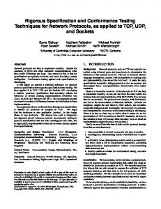
Interpretation: For determination of MSAD from TLDs it is necessary to fit measured dose values to an appropriate function for integration. For scanners without excessive field edge penumbra (most systems with rotating anode x-ray tubes), a function consisting of a square wave superimposed on a single exponential function will suffice. The width of the square wave should be equal to the measured radiation profile width (see collimation tests). Data in the field center are fitted after subtracting scatter tails fitted to single exponential with symmetry about the center of the x-ray field. This is demonstrated in Figure 2 with measured TLD data. In this case, data fit a function of the form:
where: FWHM DZ Dm a, b
= = = =
Radiation profile width at half maximum Fitted dose value at position z Mean measured dose for z within ±FWHM/2 Coefficients of fitted exponential function
IV. Summary The acceptance testing of a CT system is intended to ensure that the user receives a system with known capabilities and limitations, and which is functioning optimally at its design specifications. The methods that are described herein are designed to test all relevant aspects of system performance under conditions which best simulate anticipated clinical conditions. Tests are also designed to determine the limits of scanner performance, e.g., its highest spatial resolution, and highest contrast resolution conditions, as well as determine the compromises in radiation dose or other factors neces-
57
sary to achieve that performance level. Special attention is given to optimization of the multiformat camera image since the diagnosis is commonly done from these images. Once a system is deemed acceptable, the acceptance test data forms a benchmark for future quality assurance testing, so that any degradation in performance can be seen.
Figure 2: Measured TLD dose profile data at 1 cm depth in a head dosimetry phantom, measured with a third generation CT system, with a 10 mm slice width. The solid line represents the fitted curve. (Data courtesy of Center for Devices and Radiological Health, US FDA).
58
REFERENCES
1
NCRP Report No. 49: Structural Shielding Design and Evaluation Medical Use of X-rays and Gamma Rays of Energies Up To 10 MeV, National Council on Radiation Protection and Measurements, Washington: DC 20014, (1976). 2
Archer BR, Thornby JI and Bushong SC: “Diagnostic X-ray Shielding Design Based On An Empirical Model Of Photon Attenuation”, Health Physics, 44:507-517, (1983). 3
Simpkin DA: “Shielding Requirements for Constant Potential Diagnostic X-Ray Beams Determined by Monte Carlo Calculation”, Health Physics, 56:151-164, (1989).
4
L i n P J P : “An Interim Report of Task Group On Acceptance Testing of CT Scanners”, Works-In-Progress, Presented at the 29th Annual Meeting of AAPM, Detroit, Michigan, July 19-23, (1987). 5
Rossi RP, Lin PJP, Rauch PL and Strauss KJ: AAPM Report No.14, Performance Specifications and Acceptance Testing for X-Ray Generators and Automatic Exposure Control Devices, AIP, (1985). 6
Hanson KM: “Noise and Contrast Discrimination in Computed Tomography,” Chapter 113 in Radiology of the Skull and Brain: Technical Aspects of Computed Tomography, TH Newton and DG Potts, Editors, The C.V. Mosby Co., (1981). 7
Cohen G and DiBianca FA: “The Use of Contrast Detail Dose Evaluation of Image Quality in a Computed Tomographic Scanner,” J. Comput. Assist. Tomogr., 3:189-195, (1979). 8
B r o o k s R A a n d D i C h i r o G : “Statistical Limitation in X-ray Reconstruction Tomography”, Med. Phys., 3:237-240, (1976). 9
Haque P and Stanley JH: Detector Systems: “Basic Principles of Computed Tomography Detectors”, Section I, Chapter 118 in Radiology of the Skull
59
and Brain: Technical Aspects of Computed Tomography, TH Newton and DG Potts, Editors, The C.V. Mosby Co., (1981). 10
Riederer SJ, Pelc NJ and Chesler DA: “The Noise Power Spectrum in Computed Tomography”, Phys. Med. Biol., 23:446-454, (1978). 11
Goodenough DJ: “Psychophysical Perception of Computed Tomography Images”, Chapter 115 in Radiology of the Skull and Brain: Technical Aspects of Computed Tomography, TH Newton and DG Potts, Editors, The C.V. Mosby Co., (1981): 12
Storm E and Israel HI: “Photon Cross-sections from 1 keV to 100 MeV for Elements Z=l to Z=lOO”, Nucl. Data Tables A7,565, (1970). 13
ICRU Report 46: Photon. Electron. Proton and Neutron Interaction for Body Tissues, International Commission on Radiation Units and Measurements, (1992). 14 Joseph PM: “Artifacts in Computed Tomography”, Chapter 114 in Radiology of the Skull and Brain: Technical Aspects of Computed Tomography, TH Newton and DG Potts, Editors, The C.V. Mosby Co., (1981).
15
Hangartner TN: “Correction of Scatter in Computed Tomography Images of Bone”, Med. Phys., 14:335-340, (1987). 16
Judy PF and Swensson RG: “Display Thresholding of Images: An Observer Detection Performance Test”, J. Optical Soc. of America, A4:955965, (1987). l7
Glover GH: “Compton Scatter Effects in CT Reconstructions”, Med. Phys., 9:860-867, (1982). l8 Hemmingsson A, Jung B and Ytterbergh C: “Ellipsoidal Body Phantom for Evaluation of CT Scanners”, J. Comp. Asst. Tomogr., 7:503-508, (1983).
60
19
Johns PC and Yaffe M: “Scattered Radiation for Fan Beams”, Med. Phys., 9:231-239, (1982). 20
C a n n C E a n d G e n a n t H K : “Cross-Sectional Studies of Vertebral Mineral Using Quantitative Computed Tomography”, J. Comput. Assist. Tomogr., 6:216 (1982). 21
Yester MV and Barnes GT: “Geometrical Limitations of Computed Tomography (CT) Scanner Resolution”, Proc. SPIE, Appl. Opt. Instr. in Medicine VI, 127:296-303, (1977). 22
Joseph PM and Stockham CD: “The Influence of Modulation Transfer Shape on Computed Tomographic Image Quality”, Radiology, 145:179185, (1982). 23
Judy PF: “The Line Spread Function and Modulation Transfer Function of a Computed Tomographic Scanner”, Med. Phys., 3:233-236 (1976). 24
Bentzen SM: “Evaluation of the Spatial Resolution of a CT Scanner by Direct Analysis of the Edge Response Function”, Med. Phys., l0:579-581, (1983). 25
Droege RT and Morin RT: “A Practical Method to Measure the MTF of CT Scanners”, Med. Phys., 9:758-760 (1982).
26
Nickoloff EL and Riley R: “A Simple Approach for Modulation Transfer Function Determinations in Computed Tomography,” Med. Phys., 12:437442, (1985). 27
Kriz RJ and Strauss KJ: “An Investigation of Computed Tomography (CT) Linearity”, Proc. SPIE Appl. Opt. Instr. in Medicine VII, 555:195204, (1985). 28
Gray JE, Lisk KG, Haddick DH, Harshbarger JH, Oosterhof A, Schwenker R: “Test Pattern for Video Displays and Hard-Copy Cameras”, Radiology, 154:519-527, (1985).
61
2 9
Gray JE, Winkler NT, Stears JG, Frank ED: Qualitv Control Diagnostic Imaging, Aspen Systems, Inc., Rockville, MD (1982). 30
Shope TB, Morgan TJ, Showalter CK, et al.: “Radiation Dosimetry Survey of Computed Tomography Scanners From Ten Manufacturers”, Radiology, 146:288, (1982). 31
DHHS, FDA, 21 CFR Part 1020: “Diagnostic X-ray Systems and Their Major Components; Amendments to Performance Standard; Final Rule”, Federal Register, 49: 171 (1984). 32
Borras C, Masterson ME, Liss MM, et al.: “CT Pilot Study”, National Cancer Institutes Report, (Available from AAPM), (1985). 33
Spokas JJ: “Dose Descriptors for Computed Tomography” Med. Phys. 9:288-292, (1982). 34
J u c i u s R A a n d G X K a m b i c : “Radiation Dosimetry in Computed Tomography”, Appl. of Opt. Instr. Eng. in Med. VI, 127: 286-295, (1977). 35
Suzuki A and Suzuki MN: “Use of a Pencil Shaped Ionization Chamber for Measurement of Exposure Resulting from a Computed Tomography Scan”, Med. Phys., 5:536-539, (1978).
36
Chu RY, Fisher J, Archer BR, Conway BJ, Goodsitt MM, Glaze S, Gray JE and Strauss KJ: Standardized Methods for Measuring Diagnostic X-Ray Exposures, AAPM Report No. 31, American Institute of Physics. (1990). 37
Judy PF, Balter S, Bassano DA, McCullough EC, Payne JT and Rothenberg L: “Phantoms for Performance Evaluation of CT Scanners” AAPM report #1: American Association of Physicists in Medicine, (1977). 38
Judy PF and Adler GJ: “Comparison of Equivalent Photon Energy Calibrations in Computed Tomography”, Med. Phys, 7:685-691, (1980).
62
Appendix A SPECIFIC TECHNICAL AND PERFORMANCE INFORMATION FOR CT SCANNER BID SUBMISSION* Manufacturer: Model: Address:
Phone:
(
)
Response prepared by: Name: Title: Authorized
Signature: Date:
* Use one set of forms for each model bid.
63
A. SYSTEM ENVIRONMENTAL REQUIREMENTS 1. Electrical Power Sources: List voltage, power, and phasing for each; indicate locations on architectural drawings.
2. Power Conditioning: Give manufacturer and model numbers of power conditioning system provided:
3. Air Conditioning Requirements: Control Area:
BTU/hr
Gantry Area:
BTU/hr
Computer Room:
BTU/hr
Other
:
BTU/hr
4. Mechanical Requirements: a. Areas where raised “computer floor” is required:
b. Under-floor cable runways required: (Specify depth, width and locations on architectural drawings) c. Total weight of equipment:
lb. (kg)
Gantry:
lb. (kg)
Control Console:
lb. (kg)
64
HV Generator & Controller:
lb. (kg)
Computer System :
lb. (kg)
Other
lb. (kg)
d. Minimum floor space required (entire system):
sq.ft.(m 2 )
5. Plumbing Requirements: a Number of drains required*: b. Number of water inlets required*: *Specify location, flow rate, temperature range, etc., on architectural drawings. 6. Physical modifications: Specify the extent to which facility modifications will be performed by the vendor, with respect to installation of electrical troughs, plumbing, clinical power, air conditioning, etc.
7. Radiation Protection: Specify measured maximum exposure rate 1 meter in any direction from scan isocenter, for widest slice width and highest kVp using a cylindrical tissue equivalent phantom at least 20 cm in diameter. Kilovoltage: kVP Slice width:
mm
Phantom diameter:
cm
Phantom material: Air kerma:
mGy/mAs (mR/mAs)
65
B. SYSTEM CHARACTERISTICS 1.
X-ray Generator: a. Voltage waveform:
Continuous: pulsed:
b. kVp settings available (List):
c. mA (mAs) stations available (list for each kVp): settings at
kVp
settings at
kVp
settings at
kVp
settings at
kVp
d. Available Scan Times: Time
Scan Angle s s s s s s s
66
°
° ° ° ° ° °
2. X-ray Tube: a. Type:
Rotating anode: Stationary anode:
b. Focal spot sizes (Nominal):
Scan Plane Dimension
Axial Dimension
Focus #l
mm
mm
Focus #2
mm
mm
c. X-ray beam filtrations (operator variable - include both hardening filters and beam flattening or bow tie filters). Material
Thickness*
Intended Use
* Specify for hardening filters only. d. Thermal Characteristics: Housing cooling rate:
J/min
Anode cooling rate:
J/min
Anode heat storage capacity (cold):
J
Housing heat storage capacity:
J
Type of thermal overload protection system provided:
e. Does x-ray tube employ a mechanical shutter? 3. Beam Collimation System: a. List all available (nominal) slice thicknesses in mm:
b. Slice width settings where prepatient collimator is adjustable in axial dimension . c. Slice width settings where prepatient collimator is fixed in axial dimension . d. Slice width settings where postpatient collimator is adjustable . in axial dimension e. Slice width settings where postpatient collimator is fixed in axial dimension 4. Gantry: a. Type of Scan Motion: Rotate/translate: Symmetric fan beam, rotating detectors: Asymmetric fan beam, rotating detectors: Fan beam, stationary detector ring: Fan beam, nutating detector ring: Other: b. Variable geometric magnification available? c. Continuous rotation available?
68
d. Gantry Aperture: Maximum gantry aperture diameter:
cm
Maximum scan (sampled) diameter.
cm
e. Gantry Tilt (maximum): Gantry top toward table:
° °
Gantry top away from table: Angulation accuracy: f. Light-field Localizer: Type:
±
°
Laser: Focused Light Beam:
Configuration: Transaxial : Sagittal: Coronal: Position of transaxial localizer: At scan plane: External to scan aperture: Accuracy of transaxial localizer* ± * Coincidence of light and x-ray field centers. 5. Patient Scanning Table a. Maximum motions: Longitudinal (full out to full in):
mm
cm
Accuracy of table incrementation*
±
mm
Reproducibility* *(Table loaded with 180 lb (80 kg)
±
mm
69
Minimum table height:
cm
Maximum table height:
cm
b. Location(s) of table position indicators: Gantry: Table: Control console: Scan image: c. Table detachable from gantry? Specify cost if optional:
$
Cost of extra beds:
$
ea
°
d. Table tilt (maximum): Head end up: Head end down: Angulation accuracy: 6. Detectors a. Type: Scintillator/photodiode: Scintillator/PM tube: Type of scintillator: Pressurized xenon: Other: b. Number (exclude reference detectors):
70
° -
-
c. Efficiency: Scan Mode
Geometric (%)
kVp
Total (%)
d. Data sampling: # Projections
Scan Time
#Ray Samples*
S S S S S * Give all values if independently variable. e. Recommended calibration frequency: “Air calibration” scans: “Water calibration” scans:
71
7. Computer System: a Image reconstruction time: (measure from scan start to comple tion of display, i.e., include scan time)*.
Scan Mode
Reconstruction Scan Matrix* Time
Standard Head
Reconstruction Time
FOV s
cm
s
s
cm
s
Highest Resolution
s
cm
s
FastestScan
s
cm
s
Standard Adult Body
__
*Indicate when display matrix differs from reconstruction matrix. b. Faster reconstruction options (Specify) Option:
$
Performance (Optional conditions): Scan Mode
Reconstruction Time
Standard Head
s
Standard Adult Body
s
Highest Resolution
s
Fastest Scan
s
c. Simultaneous reconstruction and scanning?
72
d. Data storage and image archiving:
Device
MBytes
Storage Capacity* 5 1 22 2 5 62 Images Images
Raw Data Files
Magnetic tape Magnetic tape Fixed disc drive Fixed disc drive optical disc * Uncompressed data files List optional storage devices and additional cost:
Nondestructive data file compression available? Compression ratio(s): e. Convolution kernels (reconstruction filter functions): Design Purpose Name
73
Convolution kernels (continued): Design Purpose Name
g. Image display system: Pixels displayed (entire screen):
H o r i z o n t a l V e r t i c a l
Image screen size (diagonal): Operator’s console:
in(cm)
Physician’s console:
in(cm)
Gray scale bar displayed? Alphanumeric information displayed (Check where appropriate): On Separate Data Screen On Image Patient’s name: ID number: Age: Sex: Date of exam: Tie of exam:
74
Alphanumeric information displayed (cont.): on Image On Separate Data Screen Slice # kVp: mA(s): Scan time: Slice width: Bed position : Bed increment: Convolution kernel: Gantry tilt angle: Body side (R/L): h. Diagnostic software features (check if standard, give cost if op tional). Standard Cost* Feature Square region-of-interest (ROI):
$
Rectangular ROI:
$
Circular ROI:
$
Arbitrarily shaped ROI :
$
Average CT number within ROI :
$
Std. deviation of CT number:
$
Histogram of CT numbers within ROI :
$
75
Diagnostic Software Features (continued). Feature
Standard
Distance measuring utility:
Cost* $
±
Accuracy: Grid overlay:
mm $
Profile utility (CT number plot between image points):
$
Highlighting of pixels within specific CT number range:
$
Multiple image display (e.g., 2x2, 3x3):
$
Gray scale inversion :
$
Image reversal (left to right):
$
Image inversion (top to bottom):
$
Subtraction of two images:
$
Reconstruction magnification (arbitrary FOV within limits):
$
Non-reconstruction magnification:
$
High density artifact removal:
$
Programmable window settings:
$
Multi-planar
$
reconstruction:
Arbitrary angle reconstructions:
$
Dual windowing (simultaneous display of two CT number ranges):
$
76
Diagnostic Software Features (continued). Feature
Standard Cost*
Three dimensional image display:
$
Surface rendering.
$
Transparency rendering:
$
Bone mineral density measurement?
$
Dual energy material decomposition:
$
Xenon (cerebral blood flow) imaging:*
$
cardiac gating:*
$
Radii therapy treatment planning:*
$
Compiler (Fortran, C, etc.) for research programming:
$
ACR/NEMA image transfer interface:*
$
Gamma correction to match CRT phosphor to sensitivity curve of film? $ SMPTE pattern for QA:
$
Other features* (list): $ $ $ *Include cost of additional hardware required.
77
8. Hardware Accessories: (check if standard, give cost if optional). Standard Cost* Feature Head holder:
$
Infant holder
$
Flat (radiation therapy simulation) table insert:
$
Other: (specify)
$ $
9. Radiographic Scan Made: a. Projections available:
AP: Lateral: Arbitrary angle:
b. Maximum scan dimensions (at gantry axis): length:
mm
width :
mm
c. Software for scan localization from radiograph: Localization of slice positions: Accuracy:
mm
Localization of gantry (table) tilt: Accuracy:
±
78
°
10. Hard Copy Images: a Standard multiformat camera provided: (Manufacture, model)
b. Film sizes and display formats: Film size(s)
Display Format
8” x l 0 ” (20 cm x 25 cm)
1 on 1 4 on 1 9 on 1 other: 1 on 1
10” x 12” (25 cm x 30 cm)
4 on 1 9 on 1 other: 14” x 17” (35 cm x 43 cm)
4on1 9 on 1 16 on 1
other: Other film size:
79
c. Optional hard copy imaging devices available: Device
Cost $ $
$ 11. System Performance: a Specification of Performance Data: Spatial Resolution: Measured in cycles/cm at an MTF of 10%. Image Noise: Measure within an ROI of ≈1 c m2, centered within a 15-21 cm diameter cylindrical water phantom for head and pediatric scans, and a 30-32 cm phantom for adult body scans. Express as a percent of the effective linear attenuation coefficient of water, corrected for the scanner contrast scale 3 1. Radiation Dose: Specify all dose data in cGy (rads) as either multiple scan average dose (MSAD) or computed tomography dose index (CTDI), check as appropriate:
MSAD Doses must be measured at a radial depth of 1 cm in acrylic phantoms meeting specifications of the U.S. CDRH (FDA) 3 1. For all 360° scans measure at the 12 o’clock position in the phantom. Measure at mid scan arc for scans 360°.
Scan Mode
Performance Conditions: Reconstr. FOV Convol. Scan Matrix (cm) Kernel kVp Time
mAs
Slice Width
Std.Head Std. Adult Body
tõ ²…P
Best Resolution
80
scan Mode
Performance Conditions (cont): scan Reconstr. FOV Convol. Matrix (cm) Kernel kVp Time mAs
Fastest scan Lowest Noise Body Lowest Noise
ScanMode
Performance Specifications: Resolution Noise cycles/cm %SD
Std. Head Std. Adult Body Best Resolution Fastest Scan Lowest Noise Body Lowest Noise Head Pediatric Head
81
Slice Width
c. Collimation performance: Measure sensitivity and radiation profiles in mm at full width half maximum (FWHM) within a radius of 5-15 cm of gantry axis. Tolerances should reflect manufacturer’s range of acceptable error. Nominal Slice Setting
Width Tolerance
(min)
(max)
Radiation Profile Width Tolerance
±
±
±
±
±
±
±
±
±
±
±
±
±
±
C. ADMINISTRATIVE DETAILS 1. Warranties: a. Warranty Period (months beyond formal acceptance): Exclusions: x-ray tubes* Other exclusions (specify):
*If excluded, give additional cost of x-ray tube warranty during base warranty period:
$
82
b. Normal service hours:
AM to
(day) through 2.
PM, (day).
Down Time: a. Definition: Down time is defined as time when the scanner is unavailable for patient use due to failure of critical hardware or software component(s). Down time is defined over the base time period from from
AM to
PM,
(day) through
(day).
Excludes time for required preventive maintenance, component failure directly resulting from inadequate (owner- supplied) preventive maintenance or operation beyond performance specifications. % of the base b. Guarantee: Down time shall not exceed time period over any calendar month of the warranty period. c. Penalty: The warranty period will be extended by days for every 1% of down time beyond the guaranteed minimum. 3. Required Preventive Maintenance: hrs per week hrs every two weeks hrs per month 4. Service Contracts: (Use plans B and C as necessary for optional Contracts) Plan A (check all that apply) All parts excluding x-ray tubes: x-ray tubes:
83
All labor from 8:00 AM to 5:00 PM Monday through Friday: Night labor: between PM and Monday through Friday:
AM,
Weekend and holiday labor Cost: Year 1 after warranty:
$
Maximum annual increase in years 2-5 after acceptance:
%
Plan B (Check all that apply): All parts excluding x-ray tubes: x-ray tubes: All labor from 8:00 AM to 5:00 PM Monday through Friday: Night labor: between Monday through Friday:
PM and
AM,
Weekend and holiday labor: Cost: Year 1 after warranty:
$
Maximum annual increase in years 2-5 after acceptance: Plan C (Check all that apply): All parts excluding x-ray tubes: x-ray tubes: All labor from 8:00 AM to 5:00 PM Monday through Friday:
84
%
Night labor: between Monday through Friday:
PM and
AM,
weekend and holiday labor Cost Year 1 after warranty:
$
Maximum annual increase in years 2-5 after acceptance:
%
5. Maximum Service Response Time (normal business hours): hrs. 6. Other Users: If possible, provide list of names, addresses, telephone numbers and a contact person for 3 purchasers of the CT scanner model bid in this document. Name :
Telephone No.: Contact Person:
85
Name :
Telephone No.: Contact Person:
Name :
Telephone No.:
Contact Person:
86
Appendix B Phantoms for Acceptance Testing of X-Ray Transmission CT Scanning Systems It was not the intent of the Task Group on Acceptance Testing of CT Scanners to devise a “new” AAPM phantom. However, for certain tests, commercial phantoms are not always adequate or are not available. The phantoms and test objects described in this appendix include generic objects which will suffice for certain tests, as well as test objects designed specifically for this document. A. CYLINDRICAL UNIFORMITY PHANTOMS: Used for noise and uniformity measurements. All are constructed as hollow right circular cylinders, at least 2 cm in depth. Phantoms may be constructed of solid acrylic or other water simulating plastic, or may be hollow and filled with distilled water. If special phantoms are constructed, hollow phantom walls should be made of 0.5-l cm thick methyl methacrylate (acrylic) or polycarbonate, with a fill space at least 2 cm in depth. Phantom construction should exclude screws, large irregularities in wall thickness, and any artifact-producing high atomic number materials. A head phantom should have a diameter of 15-21 cm and a body phantom should have a diameter of 30-32 cm, Head and body water phantoms provided with the scanner usually suffice. An optional “baby” phantom with a diameter of 8 cm is useful for systems with large pediatric caseloads. For an inexpensive alternative, thin walled, water filled disposable plastic bottles can be used for uniformity phantoms and are often available in appropriate diameters.
87
Figure B-l: Detail of sensitivity profile test object (all dimensions are in cm unless otherwise indicated). B. SENSITIVITY PROFILE PHANTOM: This phantom incorporates a pair of 0.1 mm copper foils, inclined at an inclination ratio of 5:1 and embedded in solid acrylic blocks. As shown in Figure B-l, these blocks can be constructed as four identical and individually machined blocks, then assembled as shown, sandwiching the copper foil between. The assembled blocks are then placed within an acrylic cylinder, with a rectangular cutout to receive them. Make an annular score mark en-
88
circling the outer circumference of the cylinder, and paint the edge white to facilitate alignment with scan alignment lights.
Figure B-2: Elliptical Uniformity Phantom C. ELLIPTICAL UNIFORMITY PHANTOM: Used for uniformity measurements. This phantom is constructed as a right elliptical cylinder, with major diameters of 20 and 30 cm, as shown in Figure B-2. Two designs are acceptable. It may be constructed as a hollow water filled design with construction similar to water phantoms, and a thickness of the water space of at least 2 cm. Alternatively, it can be constructed from a solid piece of acrylic or water equivalent material (e.g., Solid Water tm Radiation Measurements Inc., Middleton, WI) with a total thickness of at least 2 cm. Optionally, for bone mineral analysis, the phantom may have a slightly oversize ≈2 cm diameter cylindrical hole placed as shown in Figure B-2. A set of inserts should then be prepared with solutions of 0, 50, 100, and 200 mg/ml of K2 H P O 4 . Alternatively the inserts could be constructed of trabecular bone equivalent plastic. An acrylic plug should be prepared to fill the hole when quantitative inserts are removed.
89
Figure B-3: Localization Image Angulation Test Object D. LOCALIZATION IMAGE ANGLE TEST OBJECT: This object, shown in Figure B-3, is designed with two pairs of thin crossed copper or steel wires on the surface of a 1 cm thick, 30 cm diameter acrylic disk. The disk is mounted on a central pivot so that it can be tilted to any arbitrary angle. The baseplate is also made of acrylic with nylon mounting screws. Wire length should be 8-10 cm and wires should be carefully aligned so that intersections of both pairs are on the same diameter, at a radius of 10 cm. Wire angles should be as depicted in Figure B-3, and may be placed in surface grooves in the acrylic disk to aid placemcnt.
90
Figure B-4: LSF Test Object E. LSF TEST OBJECT: This test object is constructed as a disk of solid acrylic which sandwiches a .076 mm (0.003”) Cu foil between the two halves so that the foil is oriented orthogonal to the scan plane. The foil should be as wide as the thickness of the disk and 3 cm long. The object is constructed from a rectangular block of acrylic, 1.5-2.5 cm thick, with sides of 20.5 cm and 20 cm. The block is cut in half, cut line parallel to the short side, and the cut surfaces are machined smooth. The copper foil is centered and glued to one of the cut surfaces of the halved block. The block is then glued back together with the foil sandwiched between. The assembly is machined into a right circular disk, 20 cm in diameter. The completed disk is shown in Figure B-4.
91
Figure B-5: Rose Phantom for CT Detail of fifth thin sheet of acetate shown, (see text). F. ROSE PHANTOM TEST OBJECT: This test object is constructed as a stack of cellulose acetate sheets, cut into 20 cm diameter circles sandwiched between a pair of l/8”, 20 cm diameter acrylic disks (to prevent the acetate from curling). Most of the test object is composed of a stack of 40 sheets of .02” (.5 mm) acetate. In the midst of this stack is a stack of 5 sheets, each .004” (0.1 mm) thick acetate. The entire stack of acetate sheets sandwiched between the acrylic disks is aligned and assembled. A series of 5 alignment holes are drilled through the stack around the periphery. The stack is disassembled and the thinner sheets are removed. Align and clamp the thin sheets between two pieces of acrylic with pins through two of the alignment holes. Mark sector hole locations, as in Figure B-5 on the acrylic sheet (becomes a template). The intent is to drill a set of live holes grouped into 10 pie shaped sectors, in a radial array
92
as shown in Figure B-5. The hole sizes within each sector are: 1 mm, 2 mm, 4 mm, 8 mm, 16 mm and 32 mm. One of the thin sheets has all sectors drilled, the fourth has eight drilled, the third six, the second four and the first two. This is done by putting the entire stack of 5 thin sheets in the template and two opposing sectors are drilled each with the live holes as shown. The top sheet is removed and the next pair of opposing sectors is drilled. This is repeated until all sectors are drilled in the final single sheet The thin sheets are then reassembled, with the holes carefully aligned. The thin stack is then sandwiched in the middle of the thick stack of acetate sheets (20 on each side), which is in turn placed between the acrylic plates. Put nylon all-thread through the alignment holes and fasten with nylon nuts. G. DOSIMETRY PHANTOMS: These phantoms are right circular cylinders of solid polymethyl methacrylate (density = 1.19 ± 0.01 g/cm 3 ), with lengths of 14-16 cm and diameters of 16 and 32 cm for the “head” and “body” phantoms, respectively (available from several dosimeter and radiological accessory manufacturers). A pediatric phantom is suggested here, for situations where pediatric scans predominate. This “infant” phantom is otherwise identical to the head and body phantoms, but with a diameter of 8 cm. All phantoms are drilled through their length for placement of dosimeters at different coaxial locations. All phantoms have holes at a depth of 1 cm (center to phantom edge) from the outer surface, at the 3, 6, 9 and 12 o’clock positions, and along the cylinder axis. Dosimeter holes at other radial locations may also be provided. Acrylic plugs provided for each hole location are removed when dosimeters are inserted.
93
Figure B-6: TLD Holder For Dosimetry Phantoms
1. TLD Holder A specially designed TLD holder suitable for sampling over a 14 cm axial distance within dosimetry phantoms is shown in Figure B-6. The holder packs 15 abutted chips over the central 14 mm of the slice, towards the edges, chips are spaced 3 mm apart. The overall length of the assembled rod (less cap) should be equivalent to that of the phantom so that the abutted chips region of the holder is centered within the phantom.
94
Figure B-7: TLD Alignment Rod for Dosimetry Phantoms 2. TLD Holder Centering Rod: This rod (Figure B-7) is identical to the acrylic plugs included with the dosimetry phantoms but at mid length there are three transverse l/16” holes 120° apart. The central hole is exactly at mid-length, while the other two holes are positioned 2.5 mm (center to center) to either side.
95