Specification of Distance Functions Using Semi-and Nonparametric Methods With An Application to the Dynamic Performance of Eastern and Western European Air Carriers1 by
Robin C. Sickles Department of Economics Rice University 6100 South Main Street Houston, Texas 77005-1892
[email protected] David H. Good School of Public and Environmental Affairs Indiana University Bloomington, Indiana 47405
[email protected] and Lullit Getachew Department of Economics Rice University 6100 south Main Street Houston, Texas 77005-1892
[email protected]
Revised September 1998, May 2000
1
Earlier versions of this paper were presented under the title of "East Meets West: A Comparison of the Productive Performance of Eastern and Western European Air Carriers." The authors would like to thank participants of the 1995 Conference on Productivity and Efficiency, Universite Catholique de Louvain, Belgium, the Wissenschaftzentrum Berlin (WZB Institute), Shawna Grosskopf, C.A.K. Lovell, Jacques Mariesse, Edwardo Rhodes and Hendrik Röller for their useful comments on previous drafts of this paper and W.W. Cooper for a lifetime of insight. The usual caveat applies.
ABSTRACT
Specification of Distance Functions Using Semi- and Nonparametric Methods With An Application to the Dynamic Performance of Eastern and Western European Air Carriers by Robin C. Sickles Rice University
David H. Good Indiana University
and Lullit Getachew Rice University
In this paper we examine the productive performance of a group of three East European carriers and compare it to thirteen of their West European competitors during the period 1977-1990. We first model the multiple output/multiple input technology with a stochastic distance frontier using recently developed semiparametric efficient methods. The endogeneity of multiple outputs is addressed in part by introducing multivariate kernel estimators for the joint distribution of the multiple outputs and potentially correlated firm random effects. We augment estimates from our semiparametric stochastic distance function with nonparametric distance function methods, using linear programming techniques, as well as with extended decomposition methods, based on the Malmquist index number. Both semi- and nonparametric methods indicate significant slack in resource utilization in the East European carriers relative to their Western counterparts, and limited convergence in efficiency or technical change between them. The implications are rather stark for the long run viability of the East European carriers in our sample.
Keywords: Distance function, stochastic frontiers, data envelopment analysis, nonparametric methods, European airline industry.
JEL Classification: C6, C14, O3, P5. 1. Introduction The European airline industry has entered a period of significant restructuring. Exempted from the competition rules of the Treaty of Rome for almost 30 years, the West European civil aviation industry faced liberalization starting
in 1986.2 At the time, the European Court of Justice ruled that the industry should be subject to competition rules in place or envisioned for other industries in the European Union. As a consequence, several waves of reforms were introduced which have led to substantial restructuring and reorganization in the industry. Even though full liberalization can hardly be expected within the next few years, air carriers are currently feeling the impact of a more competitive environment. Several carriers are going through strategic evaluations of their competitive position, not only vis-a-vis other European competitors, but also vis-a-vis carriers in the rest of the world. East European carriers are clearly going through an even more traumatic transformation. With an inability to expect large subsidies from their central governments, these airlines must prepare themselves for a more market oriented economic environment. The absorption of Interflug, the East German carrier, by Lufthansa in 1991 provides but one example that they are not up to this challenge. It is, thus, not a surprise that studies point to a gap in the level of economic activity between market and planned economies. Blanchard, et al. (1991) and Portes (1992), among others, have pointed to the disparity of economic performance in planned and market economies. Bergson (1987) examined four planned and seven market economies and found that the former had smaller capital and agricultural land productivities than the latter in 1975. Moroney (1990) found that seven East European planned economies were less efficient than seventeen West European economies during 1978-90. Moroney and Lovell (1992) reexamined the Moroney data using more sophisticated random effects stochastic frontier methods and decomposed performance into relative technical and efficiency changes. The total shortfall in productive performance between planned and market economies was estimated to be about 25% during their 1978-80 sample period, indicating considerable slack in the East European economies. Few empirical studies, however, have been carried out at the firm level. In this paper we examine the productive performance of a group of three Eastern European carriers, and compare it to thirteen of their Western European competitors during the period 1977-1990. This expands on earlier work by Good, Röller and Sickles (1993a,b, 1995), in terms of the number of carriers covered, the period under study, and the modeling framework, and complementing work by Barla and Perelman (1989).3 We model productive performance using semiparametric and nonparametric techniques. We first model the stochastic distance frontier using a semiparametric efficient estimator of a panel frontier (Park, Simar and Sickles, 1997).4 The endogeneity of multiple outputs is addressed in part by introducing multivariate kernel estimators for the joint
2
For a description of the institutional aspects of regulation and deregulation in international air transport, see de Murias (1990) or Kaspar (1991). 3
The impact of differing carrier specific institutional constraints, due to varying regulatory climates and efficiency incentives, also has been studied by Captain and Sickles (1997), Röller and Sickles (2000), Park, Sickles, and Simar (1998) for Western Europe and the U.S. during the 1970's and 1980's, and by Coelli, Perelman, and Romano (1999), Oum and Yu (1998), Good,Nadiri and Sickles (1997), and Good, Postert and Sickles (1997) for a set of international carriers through more recent periods. 4
Elsewhere, Adams, Berger, and Sickles (1999) have used such a stochastic distance function to examine efficiencies in the U. S. banking industry.
2
distribution of the multiple outputs and potentially correlated firm random effects. The semiparametric estimator is efficient within the class of estimators which make minimal assumptions about the parametric form of the stochastic structure of firm inefficiencies and other random disturbances that are usually appended to the regression model. The model imposes rather weak distributional assumptions and economic structure on the data. Details of the estimator are outlined in the Appendix. We also compare our estimates to those generated with nonparametric methods based on Data Envelopment Analysis and a Malmquist decomposition of productivity into two components--one measuring a catchup or movement to the frontier by a firm--and the other technological change--a shift in the frontier itself.5 We compare the efficiency results from these three modeling approaches by modifying the nonparametric efficiency scores to control for differences in the characteristics of the inputs of the carriers, as these are controlled for in the semiparametric stochastic frontier distance model. The paper is organized as follows. Section 2 outlines the modeling details of the three alternative constructions of productive efficiency. Section 3 describes the sample of 13 West European and 3 East European carriers which we follow with annual observations between 1977 and 1990. Section 4 discusses our empirical findings while section 5 concludes.
2. Estimation and Construction of Technical Efficiency from the Distance Function The radial measures of technical efficiency we consider in this paper are based on the output distance function.6 The goal of both the semiparametric and linear programming approaches is to identify the distance function and hence
m
D(x, y) = ∑ q ji y ji /
(1)
j
p
∑r
ki
x ki le 1
k
relative technical efficiencies. For a particular observation i, the output distance function is given by:
5
The Malmquist nondeterministic and nonparametric index number approach stands in contrast to the regression based approaches used in the macroeconomic convergence literature by, among others, Dowrick (1992). Recently, it has been modeled using time series methods by Alam and Sickles (2000) and using dynamic stochastic frontiers by Ahn, Good, and Sickles (1999, 2000) and Hultberg, Nadiri, and Sickles (1999). Recent applications using the Malmquist index have examined regulatory reform in Spanish banking (Grifell-Tatjé and Lovell, 1996), and public service production (Bjurek, Førsund , and Hjalmarrson, 1997). For recent comprehensive studies of the Malmquist index see Førsund (1997) and Färe, Grosskopf and Russell (1997). 6
Formally the Shepard output distance function is defined as:
y D( x, y ) : min λ : ∈ L( x) λ where L(x) is the set of output vectors that can be obtained with input vector x. This distance function is scalar-valued,
x, linearly homogeneous and convex in y, and non-decreasing. D(x, y) ≤ 1 if y ε L(x) and equality holds if y ∈ isoquant L(x) = {y : y ∈ L(x),θ y _ L(x), for θ > 1} (Lovell, Richardson, Travers and Wood, 1994).
decreasing in
3
where xki and yji are the levels of input k and output j, respectively. The qji and rki are weights which describe the tradeoffs among outputs and inputs that are imposed by the technology. These tradeoffs will vary from one point on the transformation function to another. A distance function takes the value of 1 if the decision making unit is productively efficient. When the firm is not efficient, the distance function describes the fraction of the efficient aggregated output, given the chosen inputs, that is actually produced by the decision making unit. As such, it provides a measure of the firm's productive efficiency. The semiparametric approach finds its roots in the distance function (1) and stresses from the outset a process where production is incompletely measured: the stochastic error term of this model incorporates measurement errors in addition to inefficiency. If we let the aggregator functions in the numerator and denominator of (1) be linearized in the natural logarithms of the outputs and inputs, then we can approximate (1) with a Cobb-Douglas distance function. An alternative form which we use in estimation is the translog distance function (c.f. Lovell, Richardson, Travers and Wood, 1994). In particular, we follow the normalization used in Lovell et al. (1994) which takes advantage of the linear homogeneity of the output distance function by renormalizing outputs in terms of one of the outputs, in our case capacity output, and placing it as a left-hand side dependent variable. We specify a translog production process which is separable in inputs (capital, labor, and network size) and outputs (revenue and capacity output) for parsimony.7 The equation we estimate then becomes
(2) where
m
m
p
p
l
j
h
k
0 = ∑∑ 12γ lj ln y l ,it ln y j ,it − ∑∑ 12 β o ,hk ln x h ,it ln x k ,it − β 1 z it − α i − ε it i = 1...N ; t = 1...T ; the z' s are conditioning variables which include time trend and variables which account
for firm heterogeneities not accounted for by the outputs and inputs; and where the effects
i
model firm differences
in efficiency. We adopt the notational conventions used by Park and Simar (1994), and Park, Sickles, and Simar (1998) in their work on semiparametric efficient estimators for generic panel models. The latter study develops the framework for estimating the sort of model in which we are interested: Namely, a panel model in which the stochastic efficiency effects are allowed to be correlated with selected regressors, in particular the y's. This ensures the endogenous treatment of multiple outputs in this regression-based distance function specification. The basic motivation for constructing a semiparametric efficient estimator of the distance frontier is to provide an improvement, in terms of a reduction in standard errors, to standard fixed effect panel treatments of (2). This is done by relying on kernel based estimates of the joint distribution of the effects and the regressors with which they are potentially correlated. In our case, all terms on the right-hand-side of (2) involving the outputs are treated as endogenous regressors which are correlated with the firm
7
The separability assumption is made to because of the curse of dimensionality problem that arises in the semiparametric estimation. In particular, the focus on the correlation between the inefficiency effect and the output ratio (a single regressor) is due to the curse of dimensionality problem of multivariate kernel density estimation in higher dimensions.
4
random effects. Essentially we are trying to soak up as much potential endogeneity in the right-hand-side outputs as possible via a Hausman-Taylor type random effects model while at the same time maintaining statistical efficiency by utilizing information that the other rgressors and the effects are orthogonal. In this particular model, it is clear that if the only source of unexplained variation that is orthogonal to the disturbance term is due to radial technical inefficiency, then by assumption it should be orthogonal to the output ratios (or their logarithms). These are what appear on the right-handside after the linear homogeneity restriction is imposed. Our estimator can be viewed as illustrative of how one could begin to bridge the gap between fully nonparametric (DEA) and fully parametric (MLE stochastic frontier) models of inefficiency. It can also be viewed as an empirical fix up to unobserved firm-specific heterogeneity that is not due to radial technical inefficiency in output levels but rather in output allocations. Ideally, a nonparametric treatment of endogenous right-hand-side output ratios would be handled by specifying multivariate kernels for the random disturbance and the appropriate regressors correlated with them. Unfortunately, the data size requirements for the proper limiting behavior of such kernels based methods are extreme (Park, et al., 1998) and are not pursued in this empirical illustration. Derivation of the semiparametric efficient estimator for the slope coefficients and the corresponding estimator for the boundary function, which leads naturally to the construction of a relative efficiency measure in terms of the distance function, is sketched in the Appendix. The effects are allowed to vary over time. We regress the estimated firm effects against a constant and time trend as in Cornwell, Schmidt and Sickles (1990). Further discussion of this type of estimator for single output stochastic panel frontier analysis can be found in Park and Simar (1994), and Park, Sickles and Simar (1998). A second frontier modeling approach is constructed by linear programming using the Data Envelopment Analysis (DEA) framework introduced by Charnes, Cooper and Rhodes (CCR) (1978). Their approach can be described in terms of the output distance function evaluated for observation i. The rationale used in DEA is to find a set of positive weights relevant to the portion of the technology for firm i which leads to the largest possible value of efficiency but is also consistent with no firm in the sample being more than 100% efficient. This criteria leads to a sequence of fractional programming problems:
(3)
max
∑q
ji
y ji
j
/ ∑r
ki
x ki
k
with respect to Ri= [r1i,...,rpi] and Qi= [q1i,...,qmi] subject to
∑q j
ji
y ji
/ ∑r
ki
x ki ≤ 1
k
The result is a piecewise linear description of the production technology which envelops all of the data. Operationally, the problem is one of obtaining the weights. CCR show that the qji and rki weights are the dual variables in the following linear programming problem for each observation, i, in the sample:
5
max φ i
φ i ,λ i ... λ NT where λ ≥ 0 subject to :
φ i yij −
(4)
∑λ
l
y jl ≤ 0 for all outputs j = 1,..., M
lnei
xki − ∑ λ l xkl ≥ 0 for all inputs k = 1...P lnei
CCR also prove that the optimal values of the linear and fractional programming problems are identical. Thus,
φi
provides a measure of the productive efficiency of the firm in observation i . While several embellishments have been made to the CCR formulation (for surveys see Charnes and Cooper, 1985, Sieford and Thrall, 1990 or Cooper, Seiford and Tone, 2000), the original formulation of the model with its constant returns to scale assumption is consistent with the vast majority of the airline literature and is not rejected in our own tests using our semimparametric model with this data.8 The panel nature of our data requires that we evaluate efficiency both across time and across firms and control for variables other than just the inputs and outputs. This is accomplished with a two step process. The first step leads to an initial evaluation of efficiency for every firm at every time period using information from all other firms and time periods to construct the weights. The subscripts and sums for firms in equation (4) are replaced with firm and time subscripts and sums. This initial evaluation of efficiency does not necessarily reflect the true performance of the firm since it excludes effects due to technological change and measurable quality variations in inputs (particularly the mix of types of airplanes in the fleets of different carriers). Consequently, the second stage projects the DEA efficiency scores on the vector of input characteristics (zi), firm specific intercepts and time variables. These yield measures of the firm specific and time varying efficiency scores as well as those of relative technical efficiency scores that are comparable to those based on the regression model introduced in section 3 above. It is important to mention that our DEA efficiencies are based on the output distance function much the same way that our semiparametric model is. We might expect then the results to be similar. They differ primarily in the way 8
Because of the complex nature of output in the air transport industry, care needs to be taken as to what scale economies mean and how they are interpreted. There are three competing ideas which have been referred to in the literature as economies of equipment size, economies of density and economies of scale. Larger aircraft are more productive than smaller ones since fixed inputs for the pilot, landing fees and terminal facilities can be spread across a larger number of passengers. These can be accommodated in our model by controlling for equipment size in the distance function. Economies of density occur when more flights, holding aircraft size fixed, are offered in individual routes. Caves, Christensen and Tretheway (1984) find that there are substantial fixed costs associated with the size of airline networks (number of cities served and average distance between those cities). Empirical work as early as Eads (1974) has suggested that economies of scale are exhausted after a carrier reaches five or six aircraft, that is, economies of scale in the production of capacity output (measured by available seat kilometers). To this discussion of the production of capacity, there are potential economies associated with how that capacity is actually filled. We might call this economies of network feed. This last feature is, in part, responsible for the international alliances formed between carriers. By funneling passengers and coordinating schedules, one partner may make the effective market size larger for the other partner.
6
that the weights in equation (1) are determined. Our semiparametric model uses global information in the determination of those weights while DEA uses only local information from observations with similar output/input mixes. This has some implications with how the technology is “filled out” where there are insufficient numbers of reference firms and involves the use of slacks, nonradial efficiency components.9 Because our semiparametric model incorporates a parametric description of the frontier, these slacks are not necessary: The reference technology is specified for all efficient or inefficient input and output combinations. Both methodologies are operationally similar in the determination of inefficiency. The DEA model identifies the convex hull of the data and, in effect, minimizes the sum of the inefficiencies. Our semiparametric model separates out stochastic movements of the frontier from inefficiencies. It attributes as much explanatory power to the measured variables as possible, minimizing a function of the residuals, which are directly related to inefficiency. As a final approach we consider the Malmquist productivity index. This method allows us to determine whether or not the gap between the inefficient and efficient carriers was being closed during the sample period. This convergence approach extends those currently used in the economic growth literature to test how productivity components of technology and efficiency have moved over our sample period in the European industry. The Malmquist productivity index procedure was introduced by Caves, Christensen and Diewert (1982) and further developed by Färe, Grosskopf, Lindgrin and Ross (1992), Färe, Grosskopf, Norris and Zang (1993) and Färe, Grosskopf and Russell (1997). These authors note that the Shephard distance function, which is the basis of the Malmquist index, and the Farrell (1957) measure of technical efficiency are reciprocals. Färe, Grosskopf, Norris and Zang (1993) show that a decomposition based on the geometric mean of two Malmquist indices can account for changes in both technical efficiency (catching up) and changes in frontier technology (innovation). The production technology, output distance function and DEA linear programming problem are amended to use only data at time t. The programming problem then becomes a series of DEA problems using only the contemporaneous information set to facilitate a comparison between the distance functions for two adjacent time periods. The distance function scales the outputs in time t+1 such that (yt+1, xt+1) is feasible in period t. It is possible that this observed input-output combination was not possible in time t, and thus the value of this expression could exceed unity, representing technical change. The output based Malmquist index is then defined as a geometric mean of two Malmquist indices, which are themselves ratios of output distance functions: (5)
D (y , x ) D (y , x ) M ( y t +1 , xt +1 , y t , xt ) = t t +1 t +1 t +1 t +1 t +1 Dt ( y t , xt ) Dt +1 ( y t , xt )
1/ 2
which has an equivalent representation as:
9
In particular, output slack occurs when a firm forms part of the envelope or efficient frontier, but in the piecewise linear construct of the frontier in DEA, the observation from the firm falls on the section of the frontier which is parallel to an axis. In this case, it is possible to increase the amount of output produced using the same amount of input. Hence, to the extent that slacks are present, the DEA gives measures which overstate technical efficiency.
7
D ( y , x ) D ( y , x ) Dt ( y t , xt ) M ( y t +1 , xt +1 , y t , xt ) = t +1 t +1 t +1 t t +1 t +1 Dt ( xt , y t ) Dt +1 ( y t +1 , xt +1 ) Dt +1 ( y t , xt )
(6)
1/ 2
= E t+1 T t+1 The first term in (6) reflects changes in relative efficiency between period t and t+1 and the second term relates changes in technology between the time periods. This index can capture productivity change by accounting for technical and efficiency advances which incorporate data from two adjacent time periods. Once the four programming problems are solved for each set of observations we can substitute these into equation (6) to obtain the Malmquist index and its two components of efficiency and frontier advances. To capture quality differences in inputs, the z-variables are also included as inputs in the linear programming problems used to calculate the Malmquist indices and their two components. Since the Malmquist index uses data from adjacent periods, there is no natural way of projecting this index on the input characteristics and time: Hence, the inclusion of the zvariables as inputs. An index less than unity indicates productivity decline while a value greater than unity indicates growth.
3. Data Our study follows sixteen European carriers with annual observations from 1977 through 1990. We have thirteen West European carriers along with thier Official Airline Guide two letter ticket designation: Air France (France, AF), Alitalia (Italy, AZ), Austrian Airlines (Austria, AU), British Airways (Great Britain, BA), Finnair (Finland, FN), Iberia (Spain, IB), KLM (Netherlands, KL), Lufthansa (Germany, LF), Olympic (Greece, OL), Sabena (Belgium, SN), SAS (Sweden, Denmark, Norway, SA), Swissair (Switzerland, SW), and TAP (Portugal, TP); and three carriers from East Europe: CSA (Czechoslovakia, CS), JAT (Yugoslavia, JA), and MALEV (Hungary, MA).10 The source of information is the International Air Transport Association's (IATA) World Air Transport Statistics (issues 1977 through 1990). This has some advantages and disadvantages when compared to data based on International Civil Aviation Organization (ICAO) information which has been used in our previous work (see, for example, Good, Röller and Sickles (1993,1995) for detailed construction of international airline data using ICAO information). The primary advantage of our data is that IATA provides systematic information on all of the carriers in our sample while ICAO systematically excludes the East European carriers. The IATA annual report provides detailed information on Association members’ physical inputs and outputs. But, unfortunately unlike ICAO, it provides virtually no information on financial variables that could be used to generate price series for inputs or outputs, or details about broad categories of inputs such as fuel or materials where measurement is based on financial data. For that reason, we 10
Except for Ireland and Luxembourg, our sample of Western European airlines includes all of the European Union (EU) member countries and also those of Finland and Switzerland. The Eastern European sample includes airlines of Hungary and Czech/Slovak Republics, which are countries that have applied for membership in the EU.
8
restrict our attention to construction of distance functions which do not require information on prices. Our assumption is that these variables are strongly correlated with other variables which are explicitly included in our model, notably the correlation between labor and materials, or that these variables may be a small factor in cost (for U.S. carriers fuel and materials expenditures comprise about 25% of total cost with the bulk of expenditures being on capital and labor). At any rate, it is not clear how meaningful such price information would be in the East European command economies. The output variables are the total revenue output and capacity output. These two measures classify output into purchased output and available output respectively. Revenue output measures passengers and cargo actually flown. Capacity output measure seats flown whether or not they are occupied by a passenger. The capacity output measure describes the potential output of the airline and provides an important measure of service quality. A carrier offering a lot of flights (and consequently having a large capacity output) will be more likely to have a seat available when a passenger wants it. Both outpus are nominally measured in tonne-kilometers with the standard assumption made that an average passenger and associated baggage weigh 100 kilograms.11 The input variables used in this study are the total number of employees, the number of aircraft, and scheduled network size (in route kilometers). Our use of network size as an input stems from the view that international air travel is not an open, competitive market. Service can be provided between two points only when bilateral agreements are negotiated between the two countries. Further, those airlines which operate more extensive networks typically must keep personnel at more diverse parts of the world, increasing their costs. A final reason for including this important variable is that it interacts importantly with capital. Previous work has shown that econonomies of route density can be important (see, Caves, Christensen and Tretheway, 1984). Network size also allows us to include one more correlate of fuel consumption as an input, minimizing the consequences of our inability to measure it directly. In addition, we construct two variables which more completely describe the nature of the fleet (proportion jet and proportion wide bodied jet). These two additional variables, which we interpret as controls for input heterogeneity, incorporate the productivity advantages of speed (with proportion jet) and the advantages of increasing returns to equipment size (with proportion wide bodied jets). Jet aircrafts lead to approximately twice the speed and consequently twice the number of revenue tone kilometers for aircrafts of the same size. Wide bodied aircrafts spread out landing slots, pilots, airport gates, fuel consumption and other factors over more passengers. Alternatively, larger aircrafts are more difficult to fill in a competitive environment. While more characteristics describing the capital stock may be useful under some circumstances, our need for parsimony, particularly with DEA models, requires we keep only the most important fleet characteristic measures. Variable means and standard deviations for the East and West European carriers in our sample are provided in Table 1.
11
Note that capacity output is a ratio of revenue output and passenger load factor. The actual equation in the SDF formulation we estimate shows that our multi-output consists of capacity output - LHS variable - and load factor - RHS variable. These two variables describe the multi-output production of an airline firm in a satisfactory way since they are not much correlated.
9
4. Estimation Results Parameter estimates from the semiparametric stochastic distance frontier are presented in Table 2 while relative efficiency scores during the sample period, exp[
it
- max(
jt)],
are presented in Table 3.12 We tested a number of
hypotheses regarding model specification. Our analysis indicated no explanatory power for the second-order terms involving input variables. Consequently, our final estimates in Table 2 are based on a functional form that is a translog model in outputs and Cobb-Douglas in inputs. We test a hypothesis of constant returns to scale and could not reject it at nominal significance levels. This is a particularly important feature in our model since Eastern European carriers tend to be much smaller than Western European carriers. Our finding of approximately constant returns to scale is consistent with the vast majority of empirical work in the airline industry over the last fifty years and our own work in a variety of aviation contexts (U.S. domestic aviation: Eads, 1972; White, 1979; Caves, Christensen and Tretheway; 1984, Sickles (1985), Alam and Sickles, 2000; Ahn, Good and Sickles, 2000; and in international aviation: Good and Rhodes, 1990, Avmark, 1992, Good, Röller and Sickles, 1993a, 1993b, 1995, and Ahn, Good and Sickles, 1999). It should be noted that our economies of scale measure is very different from economies of equipment size: We hold equipment size approximately constant by controlling for jet and wide body aircraft. Larger aircraft are more productive than smaller ones. To the extent that larger carriers have a higher tendency to employ larger planes it is a potential source of competitive advantage. Our results suggest that the size of the airline “plant” is the aircraft level and that larger airlines do not have access to different technologies, they simply replicate the same “plant” more times. To the extent that there are cost advantages associated with operating more aircraft and larger networks, they are offset by increasing complexities in network and managerial coordination. Our efficiency modeling describes the supply side of the industry only, and does not preclude advantages which operate on the demand side of the market. For example, the strategic alliances which are common in the industry do nothing to alter the carrier’s cost of providing service. These alliances can have a major effect in increasing the demand for services at a point where the carriers connect. We also tested for and rejected at nominal significance levels heterogeneity as well as non-linearities in technical change for the East and West European carriers and thus have proxied technical change with a single time trend. Heterogeneity controls for the inputs, the z variables in equation (2), are the proportions of a fleet which utilizes wide bodied aircraft (PWIDEB) and jet aircraft (PJET), with the omitted category being the proportion of a fleet that is turboprop aircraft. The parameter estimates of the three heterogeneity controls based on the DEA method are 0.013 for time trend, 0.420 for PWIDEB and -0.0864 for PJET with t-statistics of 6.84, 5.58 and -1.29 respectively. The DEA programming estimates of efficiency and relative scores are presented in Table 4. The Malmquist indices and their decomposition into the technical and efficiency change components are presented in Tables 5, 6, and 7. Our findings point to substantial agreement between the semiparametric stochastic distance frontier (SDF)
12
The parameter estimates from the SDF given in Table 2 can be interpreted as input and load factor elasticities of capacity output.
10
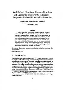
estimates of firm technical efficiency and those from conventional DEA programming methods. This is not surprising given the radial nature of our efficiency measurement and the reliance of both techniques on the output distance function. Lufthansa and KLM are the most efficient while CSA and MALEV are the least efficient with the remaining twelve firms in between, some showing quite similar levels. It is also sensible that JAT, the Yugoslavian carrier, is the most efficient among the East European airlines since its form of socialism was quite different from either Hungary or Czechoslovakia. This finding may also be a result of JAT having access to western equipment; they could purchase Boeing and McDonnel-Douglas aircraft while other Eastern European carriers were politically prohibited from doing so. One interesting discrepancy between the SDF and DEA estimates is the temporal pattern of efficiency change for British Air, where the two methods registered a relative efficiency of about 60% and 70% in 1977, but only the SDF estimates showed the dramatic efficiency gains from privatization by 1990. Figures 1 and 2 show the relative difference in levels and the relative comparability in temporal patterns for SDF and DEA efficiency scores during the sample period for the East and West European carriers. Taken together, the results point to a relatively wide gap in the technical efficiencies between the Eastern and Western firms of about 45% in 1977 and decreasing to only 43% in 1990. The dynamics of potential catching-up and convergence of the productivity of East European carriers to that of their more efficient West European competitors can be examined by focusing on the nonparametric Malmquist index and its decomposition. The indices are constructed so that values larger than one indicate progress while those less than one indicate regress. Figures 3, 4 and 5 display the temporal patterns of the Malmquist index and its decompositions. On average, results indicate that the efficiency and technical change components for East European carriers are slightly below those for their Western counterparts at the beginning of the study period and that this pattern was rather stable over the sample period; the malmquist index averages to 0.9557 over the12 year period for the East European carriers compared to 1.0176 for the Western airlines. Moreover, East European carriers had an annual technical change which was somewhat below that for the Western firms, 0.9846 versus 1.0177. The se figures are, however, close enough which is not surprising given the ubiquitousness of the technology of commercial aviation and its rapid international diffusion; for example, JAT's fleet consisted of Boeing and McDonnell-Douglas aircraft during the study period. These results of efficiency and technical change point to little change in the relative position of the two European airline industries. Together with the other two methodologies, they point to a substantial disparity in technical efficiency differences between the East and West commercial airline industries, averaging about 43% in 1990, the end of the sample period, and suggesting substantial underutilization of productive resources in the East. A large reservoir of commercial airline service could be launched by the East European firms if they implement the market incentives and organizational changes contemplated by, or already in place in, their West European counterparts. Even with a robust growth of 2% per year, the East European airlines could provide service through the early next century with the factor inputs in place. Alternatively, a 30% reduction in labor force in the commercial airline industry could put the East European carriers in a productively competitive posture vis-a-vis Western Europe. The wrenching changes in labor markets under way in the former East Germany, for example, point to unemployment rates in excess of 20% as a result of integration with West Germany and imply a rather stark future for East Europe. Our results point to comparable
11
reallocation in other East Europan countries for one of its most most modern and technological industries, its commercial aitr transportation industry.
5. Conclusions In this study we have outlined a general methodology which can be employed to examine the productive performance of multiproduct technologies. The statistical method, which has previously been applied to estimate stochastic frontier production functions, has been extended here to handle multi-output distance function estimation as well. The programming alternatives, DEA and the Malmquist index, are approaches which have been used extensively to model productive performance in multi-product technologies. Their use has often been motivated on the basis of not requiring the price data necessary to estimate parametric multi-output technologies through the dual cost function. Our semiparametric stochastic distance frontier, besides extending prior statistical methods to estimate multi-output distance functions, reveals differences in productive performance at the firm level between East and West European carriers. Our study also expands on previous studies of efficiency by covering the performance of more carriers over longer periods. Our new estimator, along with the DEA and Malmquist index number approaches, uncovers a disparity in productive performance between West and East European airline firms suggesting substantial slack in resource utilization by the Eastern carriers. The implications of our analysis are rather stark. Either the East European carriers adopt a more rational production strategy or receive increasing subsidies, which will place further strains on already financially stretched national economies. Appendix Assume there are N independent observations (X*i , Yi), where X*i' = ( xi1 ,....,xiT ,zi1,...,ziT)' and Yi' = (y1,i1 ,..., y1,iT , where Yi* contains terms involving all outputs except the level of the first dependant variable which is moved to the left-hand-side of (2); Xi* and Y*i are i.i.d. (L x T) and (M-1 x T)-dimensional random vectors. The Xi* have an Yi*)',
β = (β o , β 1 ) and γ * are (Lx1) and (M-1 x 1)-dimensional unknown vectors of parameters. The ( α i i, Y*i) are i.i.d. from unknown distribution h and ε it are considered i.i.d. random variables from N(o, σ 2) with unknown σ 2. The support of the marginal density of α i i is considered bounded from above. Let ( α ,Y)
unknown density function g;
denote generic observations from ( α i ,Yi*) and
T
1 * Y = T ∑ Y i . Consider the joint distribution h and assume the *
i=1
following form:
(a.1) α
h( α ,Y * ) = h M ( α ,Y * )p( Y * )
where hM is the joint density function of
( α ,Y * ) and p(Y*) is an arbitrary function. This distribution assumes that *
changes in Y* depend on only through changes in Y , through long run changes in Yi*. In other words, firm specific effects depend only on the long run mix of product outputs. To derive the semiparametric efficient estimator for the distance function (2) we need to first derived the information bound. Let (X*,Y) represent a "generic" observation and θ = ( β , γ ) . Let P represent the set of all possible joint distributions of (X*,Y). Consider a regular subset P0 of all the possible joint distributions endowed with *
12
L( X * ,Y,θ ,η ) denote the log likelihood of an observation from * * P( θ ,η ) and lθ ( X ,Y) and lη j ( X ,Y) be the derivative of the log likelihood function with respect to θ and the vector of nuisance parameters η . The information bound for θ is then given by: a set of regularity conditions discussed therein. Let
(a.2)
I(P;θ , P0 ) = E p l* l* ′ ( X * ,Y)
* l = lθ - Π( lθ | lη ) where and the notation Π( l | [ lη ]) denotes the vector of projections of each component of l onto the space l in L2(P),
(a.3)
that is, based on the least squares projections. The information bound for equation (2) above is gotten by first letting St( θ ) = y1,t - X*t - Yt* * and Ut=St( ) - S t ( θ ) , where T
-1 S t ( θ ) = T ∑ S t ( θ ). t =1
Next let
(a.4)
(a.5)
ω ( z1 , z 2 ) = ∫ φ σ ( z1 - u) h M (u, z 2 )du = φ*σ h M (., z 2 )( z1 )
Io= ∫
( ω ′ )2 ( z1 , z 2 ) dz 1 d z 2 ( ω )2
σ , and T be the Fisher information for location of ω , where ω ' is the derivative with respect to the first component of the vector. be the joint density of
( S t , Y * ) , where σ =
T
(a.6)
* * * 1 * * ΣW ( X ) = E p T ∑ ( X t − X )( X t − X )′ t =1
T
(a.7)
* * * * * 1 Σ B ( X ) = E p T ∑ ( X − E p ( X ))( X − E p ( X ))′ t=1
T
(a.8) (a.9)
* * * 1 * * ΣW ( Y *) =*E p T ∑ 1( YT t − Y* )( Y* t − Y * )′ * ΣW ( X ,Y ) = E pt=1 T ∑ ( Y t − Y )( X t − X )′ t=1
Consider the within and between covariances, which are defined as follows:
13
* * * ΣW ( X ) ΣW ( X ,Y ) ΣW = ( * , * )′ * ΣW ( Y ) ΣW X Y
(a.10)
T
where
1 * X = T ∑ X t . Assume that I0 < ∞ and ΣW (X) and Σ B (X) both exist and are nonsingular. In this model the *
t =1 *
*′ *′ l = ( lβ ,lγ * )′ and information bound can be obtained by maximizing the log likelihood function with * respect to β and γ and then by subtracting the conditional expectations of these derivatives from the actual derivative
efficient score
T
(a.11)
l* β = σ 2 ∑U t X *t ( X * E p ( X * )) t =1
ω′ ( S ,Y * ) ω
T
(a.12)
l*γ * = σ 2 ∑U tY *t t =1
to get the efficient score function (Theorem 2.1, Park and Simar, 1994):
0 σ 2 ΣW ( X * ) + I 0 Σ B ( X * ) . (a.13) I = 2 * 0 σ ΣB ( Y ) To construct an estimator of ω we use the logistic kernel estimator, (a.14)
N
J
i=1
j= 2
ω ( t 1 , t 2 , ..., t j+1 ;θ ) = N -1 ∑ K S N ( t 1 - S i )∏ K S N ( t j+1 - Y *ji )+ o p (1) -t
-t -2
where Ks = K(t/s)/s, K(t) = e (1+ e ) . Define the estimate of
∑ ∑U~ ( θ ) N
(a.15)
σ~ 2 ( θ ) =
T
2 it
i=1 t =1
N(T 1)
14
σ 2 and the between covariance as:
T
* ~ ΣB ( X ) =
(a.16)
N
where
T
∑( X
* t
* * * X )( X t X )′
t =1
N
* it
X is the population mean. The efficient estimator is now defined by: * X = ∑∑ i=1 t=1 (NT)
* ~ ~ * ~2 0 ~ T ΣW ( X )/ σ + I o Σ B ( X ) I= 2 ~ * ~ 0 T ΣW ( Y )/ σ
(a.17 ) and where
~ θ N is any consistent estimator, and where any expression superscripted by "~" has been evaluated at this
initial consistent estimator. In our empirical work we use the within estimator of Cornwell, Schmidt and Sickles (1990) as the initial consistent estimator and the bootstrap method for selecting the bandwidth in constructing the multivariate kernel density estimates in eq. (16) discussed in Park and Simar (1994) and Park, Sickles and Simar (1998).
(a.18)
αˆ i = S i ( θˆ N,T ) Given the efficient estimator
θˆ N,T ,
i
are predicted by:
Under the assumptions of the model above Park and Simar prove that as T and T
(a.19)
2 N,T
go to infinity:
L P = ( T ( αˆ i α i ) → N(0,σ ). 2
Relative technical inefficiencies of the i-th firm with respect to the j-th firm can be predicted by: αˆ i interested in firm relative efficiencies with respect to the most efficient firm:
15
max j=1,...,N ( αˆ j ) .
αˆ j . We are most
References
Adams, R. A., Berger, A., and R. C. Sickles (1999), “Semiparametric approaches to stochastic panel frontiers with applications to the banking Industry,” Journal of Business and Economics Statistics 17: 349-358. Ahn, S., D. Good, and R. C. Sickles (1999), “Assessing the relative efficiency of Asian and North American airline firms,” Economic Efficiency and Productivity Growth in the Asia Pacific Region, Tsu-tan Fu, Cliff J. Huang, C. A. K. Lovell (eds.), UK: Edward Elgar Publishing Limited: 67-94. Ahn, S., D. Good, and R. C. Sickles (2000), “Estimation of long-run inefficiency levels: a dynamic frontier approach”, Econometric Reviews, forthcoming. Aghion, P. (1993), "Economic reform in Eastern Europe," European Economic Review 37, 525-532. Alam, I. S., and R. C. Sickles (2000), “Time series analysis of deregulatory dynamics and technical efficiency: the case of the U. S. airline industry, International Economic Review 41, 203-218. Avmark (1992), The Competitiveness of the European community’s Air Transport Industry, prepared for the Commission of the European Communities. Barla, P. and S. Perelman (1989), "Technical efficiency in airlines under regulated and deregulated environments," Annales de l'Economie Publique Sociale et Cooperative 60, 61-80. Bergson, A. (1987), "Comparative productivity: the USSR, Eastern Europe, and the West," American Economic Review 77, 342-57. Blanchard, O., R. Dornbusch, P. Krugman, R. Layard and L.Summers (1991), Reform in Eastern Europe, M.I.T. Press, Cambridge, MA. Bjurek, H., Førsund, F. R., and L. Hjalmarrson (1997), “Malmquist productivity indexes: an empirical comparison,” in Index Numbers; Essays in the honor of Sten Malmquist, R. Färe, S. Grosskopf, and R. R. Russell (eds), Boston: Kluwer Academic Publishers. Captain, P., and R. C. Sickles (1997), “Competition and market power in the European airline industry: 1976-1990,” Managerial and Decision Economics 18(3),209-225. Caves, D.W., L.R. Christensen and W.E. Diewert (1982), "Output, input and productivity using superlative index numbers," Economic Journal 92, 73-96. Caves, D.W., L.R. Christensen and M.W. Tretheway (1984), "Economies of density versus economies of scale: Why trunk and local service airline costs differ," The Rand Journal of Economics 15: 471-489. Charnes, A., and W.W. Cooper (1985), "Preface to topics in data envelopment analysis," Annals of Operations Research 2, 95-112. Charnes, A., W.W. Cooper, and E.L. Rhodes (1978), "Measuring the efficiency of decision making units," European Journal of Operational Research 2, 429-444. Coelli, T., S. Perelman, and E. Romano (1999), “Accounting for environmental influences in stochastic frontier models with application to international airlines,” Journal of Productivity Analysis 11: 251-273.
16
Cooper, W. W., L. M. Seiford and K. Tone (2000) Data Envelopment Analysis Boston: Kluwer Academic Publishers. Coricelli, F. and G. M. Milesi-Ferretti (1993), "A note on wage claims and soft budget constraints in economies in transition," European Economic Review 37, 387-395. Cornwell, C., P. Schmidt and R.C. Sickles (1990), "Production frontiers with cross-sectional and time-series variation in efficiency levels," Journal of Econometrics 46, 185-200. Dewatripoint, M., and G. Roland (1992), “The virtues of gradualism and legitimacy in the transition to a market economy," Economic Journal 102, 291-300. Dowrick, S. (1992), "Technological catch up and diverging incomes: patterns of economic growth 1960-1988," Economic Journal 102, 600-610. de Murias, R. (1990), The Economic Regulation of International Air Transport. Jefferson, NC: McFarland and Company. Eads, G.C. (1972), The Local Service Airline Experiment. Washington, D.C.: Brookings Institution. Färe, R., S. Grosskopf, B. Lindgren, and P. Ross (1992), "Productivity changes in Swedish pharmacies 1980-1989: a non-parametric Malmquist approach," Journal of Productivity Analysis 3, 85-101. Färe, R., S. Grosskopf, M. Norris, and Z. Zhang (1993), "Productivity growth, technical progress, and efficiency change in industrialized Countries," American Economic Review 84, 66-83. Färe, R., S. Grosskopf, and C. A. K. Lovell (1994), Production Frontiers, New York: Cambridge University Press. Färe, R., S. Grosskopf, and R. R. Russell (eds.) (1997), Index Numbers; Essays in the Honor of Sten Malmquist, Boston: Kluwer Academic. Farrell, M. J. (1957), “The measurement of productive efficiency,” Journal of the Royal Statistical Society Series A, 120(3) pp253-282. Førsund, F. R. (1997) “The Malmquist Productivity Index, TFP and Scale,” University of Oslo, mimeo. Good, D. H., M.I. Nadiri, L.-H. Röller and R. C. Sickles (1993a) "Efficiency and productivity growth comparisons of European and U.S. air carriers: a first look at the data," Journal of Productivity Analysis 4, J. Mairesse and Z. Griliches (eds.), 115-125. Good, D. H., L.-H. Röller, and R. C. Sickles (1993b), “U. S. airline deregulation: implications for European transport," Economic Journal 103, 1028-1041. Good, D. H., L.-H. Röller, and R. C. Sickles (1995), “Airline efficiency differences between Europe and the U.S.: implications for the pace of E. C. integration and domestic regulation," European Journal of Operations Research 80, 508-518. Good, D. H., M. I. Nadiri, and R. C. Sickles (1997a), “Index number and factor demand approaches to the estimation of productivity,” Handbook of Applied Econometrics, Volume II-Microeconometrics, Chapter 2, M. H. Pesaran and P. Schmidt (eds.), Cambridge, UK: Basil Blackwell, 14-80. Good, D. H., A. Postert, and R. C. Sickles (1997b), “A model of world aircraft demand,” mimeo. Grifell-Tatjé, E., and C. A. K. Lovell (1996), “Deregulation and productivity decline: the case of Spanish savings banks,”
17
European Economic Review 40, 1281-1303. Hughes, G. and P. Hare (1992), "Industrial restructuring in eastern Europe," European Economic Review 36, 670-676. Hultberg, P., M. I. Nadiri, and R. C. Sickles (1999), “An International Comparison of Technology Adoption and Efficiency: A Dynamic Panel Model,” Annales D’Économie et de Statistique, Special Issue in Commemoration of the 20th Anniversity of the Panel Data Conference, (ed.) Patrik Sevestre: 55-56: 449-474. Kaspar, D.M. (1991), Deregulation and Globalization: Liberalizing International Trade in Air Services, Cambridge MA: Ballinger Publishing Co. Lovell, C. A. K., S. Richardson, P. Travers, and L. Wood (1994), "Resources and functionings: A new view of inequality in Australia, in Models and Measurement of Welfare and Inequality, W. Eichhorn (ed.), Heidelberg: SpringerVerlag, 787-807. Moroney, J. R. (1990), "Energy consumption, capital, and real output: a comparison of market and planned economies," Journal of Comparative Economics 14, 199-220. Moroney, J. R., and C. A. K. Lovell (1992), "The performance of market and planned economies revisited," mimeo. Oum, T. H., and C. Yu (1998), “Cost competitiveness of major airlines: an international comparison,” Transportation Research Part A 32(6), 407-422. Park, B., and L. Simar (1994), "Efficient semiparametric estimation in stochastic frontier models,” Journal of the American Statistical Association 89, 929-936. Park, B., R. C. Sickles, and L. Simar (1998), "Stochastic panel frontiers: a semiparametric approach," Journal of Econometrics, 84, 273-301. Portes, R. (1992), "Structural reform in central and eastern Europe," European Economic Review 36, 661-669. Röller, L.-H., and R. C. Sickles (2000) “Capacity and product market competition: measuring market power in a ‘puppydog’ industry,” forthcoming in the International Journal of Industrial Organization. Roland, G. (1993), "The political economy of restructuring and privatization in eastern Europe," European Economic Review 37, 533-540. Sickles, R. C. (1985), “A Nonlinear Multivariate Error-Components Analysis of Technology and Specific Factor Productivity Growth with an Application to the U. S. Airlines,” Journal of Econometrics 27, 61-78. Sieford, L., and R. M. Thrall (1990), "Recent developments in DEA: the mathematical approach to frontier analysis," Journal of Econometrics 46, 7-38. Taneja, N.K. (1988), The International Airline Industry, Lexington, MA: Lexington Books. White, L.J. (1979), “Economies of scale and the question of natural monopoly in the airline industry,” Journal of Air Law and Commerce, 44: 545-573. Wyploz, C. (1993), "The transformation of eastern Europe: macroeconomic issues," European Economic Review 37, 379-386.
18
Table 1 Summary Statistics For the Eastern and Western Airline Firms
EASTERN EUROPE _________________________________________________________________ Variable Mean Std. Dev. _________________________________________________________________ Revenue Output Capacity Output Number of Planes Labor(workers) Network Size Proportion Jet Aircraft Proportion Wide Body
249,167.73 381,988.14 35.94 5,942.08 109,713.24 0.770 0.030
142,326.71 212,459.25 10.22 1,099.08 37,255.09 0.235 0.045
WESTERN EUROPE ________________________________________________________________ Variable Mean Std. Dev. ________________________________________________________________ Revenue Output Capacity Output Number of Planes Labor(workers) Network Size Proportion Jet Aircraft Proportion Wide Body
2,097,418.49 3,239,202.99 67.42 18,804.08 304,470.75 0.931 0.257
19
1,887,366.54 2,793,744.67 44.01 12,726.94 217,803.28 0.104 0.157
Table 2 Semiparametric Efficient Parameter Estimates of the Stochastic Distance Frontier
Variable
Parameter Estimate
Standard Error
T-Statistic (Ho: Parameter=0)
ln(Revenue Output)
1.712
0.5180
3.31
ln(Rev. Output)2
0.864
0.4881
1.77
ln(Planes)
-0.151
0.0628
-2.40
ln(Labor)
-0.675
0.0663
-10.2
ln(Network)
-0.175
0.0465
-3.76
PWideB
-0.273
0.1222
-2.23
PJet
0.802
0.1071
0.75
Time trend
-0.036
0.0055
-6.45
Adjusted R2 = 0.998
20
Table 3 Stochastic Distance Frontier Relative Efficiencies Year 1977 1978 1979 1980 1981 1982 1983 1984 1985 1986 1987 1988 1989 1990
AF 0.91661 0.91152 0.90646 0.90143 0.89642 0.89145 0.88650 0.88158 0.87669 0.87182 0.86698 0.86217 0.85739 0.85263
AU 0.43650 0.42991 0.42342 0.41702 0.41072 0.40451 0.39840 0.39238 0.38646 0.38062 0.37487 0.36920 0.36363 0.35813
AZ 0.77787 0.77551 0.77315 0.77080 0.76845 0.76611 0.76378 0.76146 0.75914 0.75683 0.75453 0.75224 0.74995 0.74767
BA 0.73680 0.75015 0.76375 0.77759 0.79168 0.80603 0.82064 0.83552 0.85066 0.86608 0.88177 0.89776 0.91403 0.93059
CS 0.20834 0.20786 0.20738 0.20690 0.20642 0.20594 0.20546 0.20499 0.20451 0.20404 0.20357 0.20309 0.20262 0.20215
FN 0.37153 0.37523 0.37896 0.38274 0.38654 0.39039 0.39427 0.39820 0.40216 0.40616 0.41020 0.41428 0.41841 0.42257
IB 0.62596 0.62203 0.61813 0.61425 0.61039 0.60656 0.60275 0.59897 0.59521 0.59147 0.58776 0.58407 0.58040 0.57675
JA 0.41938 0.41858 0.41779 0.41700 0.41620 0.41541 0.41462 0.41384 0.41305 0.41227 0.41148 0.41070 0.40992 0.40914
Year
KL
LF
MA
OL
SA
SB
SW
TP
1977
0.99135
1.00000
NA
0.54652
0.77396
0.75606
0.79248
0.41011
1978
0.98977
1.00000
NA
0.53288
0.75012
0.76205
0.78210
0.40931
1979
0.98820
1.00000
NA
0.51958
0.72702
0.76809
0.77186
0.40852
1980
0.98663
1.00000
NA
0.50662
0.70463
0.77418
0.76176
0.40774
1981
0.98506
1.00000
NA
0.49398
0.68294
0.78314
0.75178
0.40695
1982
0.98349
1.00000
NA
0.48165
0.66190
0.78649
0.74194
0.40616
1983
0.98193
1.00000
NA
0.46964
0.64152
0.79273
0.73223
0.40538
1984
0.98037
1.00000
0.19093
0.45792
0.62177
0.79901
0.72264
0.40460
1985
0.97881
1.00000
0.18814
0.44649
0.60262
0.80534
0.71318
0.40381
1986
0.97725
1.00000
0.18540
0.43535
0.58406
0.81172
0.70384
0.40303
1987
0.97570
1.00000
0.18270
0.42449
0.56607
0.81815
0.69463
0.40226
1988
0.97415
1.00000
0.18003
0.41390
0.54864
0.82464
0.68553
0.40148
1989
0.97260
1.00000
0.17741
0.40357
0.53175
0.83117
0.67656
0.40070
1990
0.97105
1.00000
0.17482
0.39350
0.51537
0.83776
0.66770
0.39993
21
Table 4 DEA Relative Efficiencies Year 1977
AF 0.77331
AU 0.37319
AZ 0.69636
BA 0.55862
CS 0.16354
FN 0.39872
IB 0.71604
JA 0.28152
1978
0.77592
0.37894
0.68677
0.54579
0.15969
0.38252
0.71150
0.30134
1979
0.77992
0.37957
0.68569
0.55026
0.15927
0.37371
0.70346
0.33208
1980
0.78787
0.38578
0.68936
0.55530
0.16103
0.37415
0.71081
0.33953
1981
0.81495
0.39534
0.73555
0.57647
0.17295
0.39614
0.72444
0.34975
1982
0.85845
0.40919
0.76770
0.60757
0.18955
0.40379
0.73484
0.35721
1983
0.86195
0.41720
0.76852
0.62016
0.20781
0.42678
0.74635
0.36164
1984
0.85570
0.42779
0.76207
0.62756
0.18478
0.43899
0.75673
0.36696
1985
0.85405
0.43431
0.76354
0.62647
0.20071
0.44113
0.76352
0.38689
1986
0.85598
0.43645
0.76917
0.63186
0.20693
0.44519
0.77295
0.39870
1987
0.84146
0.43049
0.68838
0.61357
0.20664
0.44702
0.76336
0.39488
1988
0.88422
0.46385
0.69783
0.60426
0.21678
0.45921
0.77076
0.41340
1989
0.92638
0.48912
0.70659
0.59544
0.22592
0.46940
0.77813
0.43952
1990
0.96214
0.50423
0.71123
0.58350
0.23783
0.47286
0.78086
0.42401
Year
KL
LF
MA
OL
SA
SB
SW
TP
1977
0.90002
1.00000
NA
0.64605
0.71715
0.90115
0.60943
0.33387
1978
0.88498
1.00000
NA
0.63464
0.70727
0.88744
0.60021
0.30902
1979
0.86905
1.00000
NA
0.64314
0.69728
0.89221
0.59444
0.29827
1980
0.87278
1.00000
NA
0.67370
0.69562
0.90028
0.60299
0.31586
1981
0.88053
1.00000
NA
0.68348
0.71283
0.90313
0.63604
0.33093
1982
0.89529
1.00000
NA
0.69321
0.72078
0.91811
0.66562
0.35219
1983
0.89787
1.00000
NA
0.71461
0.72256
0.92643
0.69321
0.35957
1984
0.89965
1.00000
0.22476
0.72754
0.72492
0.93329
0.70192
0.37459
1985
0.89697
1.00000
0.21915
0.75132
0.72722
0.94458
0.72035
0.38412
1986
0.90843
1.00000
0.21849
0.73875
0.73694
0.94265
0.73069
0.39299
1987
0.87414
1.00000
0.21569
0.71993
0.69297
0.97967
0.72695
0.39192
1988
0.86616
1.00000
0.22275
0.71316
0.71986
0.98852
0.71635
0.44714
1989
0.85860
1.00000
0.22637
0.71474
0.72591
0.99710
0.71347
0.48928
1990
0.84648
0.99460
0.23610
0.73380
0.72607
1.00000
0.71659
0.49776
22
Table 5 Malmquist Indices Year
AF
AU
AZ
BA
CS
FN
IB
JA
1977 - 1978
0.87112
0.83599
0.96608
0.79797
0.73020
0.95601
1.07885
1.08334
1978 - 1979
0.98497
0.87405
0.95060
1.02008
0.85488
0.98614
1.04658
1.01011
1979 - 1980
0.9613
0.92670
1.08677
0.86952
0.67552
1.07840
0.99573
0.99959
1980 - 1981
0.97246
0.94102
0.96479
0.86418
0.75952
1.04957
0.83609
0.98703
1981 - 1982
1.00851
0.98674
0.98812
0.85987
0.67388
1.07417
0.88064
0.97230
1982 - 1983
0.95725
0.96825
1.06860
0.94910
0.88420
1.06930
0.93768
0.98565
1983 - 1984
1.01175
1.00391
1.06473
1.05589
1.06450
0.95366
1.04121
1.06971
1984 - 1985
0.98433
0.96395
1.20726
1.01696
1.05042
1.05960
1.06711
1.13626
1985 - 1986
1.04417
1.03044
1.07337
1.01410
1.00295
1.03838
1.00021
1.07675
1986 - 1987
0.99682
1.03007
0.90936
1.01591
1.02309
1.03975
1.04310
1.04575
1987 - 1988
1.03164
1.03317
1.04108
1.11547
0.98466
1.04933
1.15844
1.00837
1988 - 1989
1.02794
1.05886
1.04488
1.10697
0.98479
1.01908
1.15348
1.02680
1989 - 1990
0.99791
1.07031
1.00744
1.07944
0.85619
1.15208
1.04331
0.94261
MA
OL
1977 - 1978
Year
0.94433
KL
0.89312
LF
NA
1.19132
1.01850
1.06133
1.06329
1.26228
1978 - 1979
0.95342
0.98429
NA
1.21625
0.95735
1.13275
0.99963
1.01440
1979 - 1980
1.06733
0.97576
NA
1.12799
0.95438
0.95851
1.02448
0.95022
1980 - 1981
1.00118
0.96281
NA
0.94916
0.93272
0.96695
1.04603
0.77178
1981 - 1982
1.07383
0.97692
NA
0.95329
0.95725
1.12418
1.04579
0.99024
1982 - 1983
1.02736
0.98363
NA
0.95689
1.00373
1.07906
1.04110
1.03529
1983 - 1984
0.99330
1.07294
NA
1.01358
1.11435
1.01339
1.02495
1.11058
1984 - 1985
1.09480
0.98563
0.92854
0.94879
0.95581
1.04171
0.97803
1.01864
1985 - 1986
0.97647
1.09847
1.02103
0.95793
1.07085
0.97780
0.96982
1.05381
1986 - 1987
1.03157
0.91496
1.03660
0.97802
1.09119
0.90953
1.10518
1.07471
1987 - 1988
1.12286
1.03514
0.98035
0.91543
0.99704
1.23215
1.02767
1.08049
1988 - 1989
1.02000
1.03196
0.98928
0.97647
1.00808
1.26658
1.04773
1.13259
1989 - 1990
1.01137
1.02035
1.08814
1.10843
0.99655
1.22395
1.01539
0.98182
23
SA
SB
SW
TP
Table 6 Efficiency Change Component of the Malmquist Index Year
AF
AU
AZ
BA
CS
FN
IB
JA
1977 - 1978
1.00000
1.00000
0.95327
1.00000
1.00000
0.89481
1.02336
1.06301
1978 - 1979
1.00000
1.00000
0.91915
1.00000
1.00000
0.94285
0.97652
1.05101
1979 - 1980
1.00000
1.00000
1.01537
1.00000
1.00000
1.01790
0.98544
0.92935
1980 - 1981
1.00000
1.00000
0.94359
1.00000
1.00000
1.00560
0.92421
0.94875
1981 - 1982
1.00000
1.00000
0.92408
1.00000
1.00000
1.00741
0.92345
0.91354
1982 - 1983
1.00000
1.00000
1.05602
1.00000
0.70076
1.04555
0.88265
0.95838
1983 - 1984
1.00000
1.00000
0.99765
0.97930
0.84519
0.91429
0.92688
1.00799
1984 - 1985
1.00000
1.00000
1.18676
1.02113
0.97215
1.06882
1.07032
1.11479
1985 - 1986
0.99086
1.00000
0.94841
0.94752
1.00000
0.91764
0.87484
0.97535
1986 - 1987
1.00922
1.00000
0.96601
1.05539
1.00000
1.06822
1.09449
1.04322
1987 - 1988
1.00000
1.00000
0.98634
1.00000
1.00000
1.02460
1.13362
0.98153
1988 - 1989
1.00000
1.02584
1.02071
1.00000
1.00000
0.99731
1.15036
0.99761
1989 - 1990
1.00000
1.00972
1.02694
1.00000
1.00000
1.16126
1.02637
0.87717
Year
KL
LF
MA
OL
SA
SB
SW
TP
1977 - 1978
1.00000
1.00000
NA
1.11622
1.01496
1.02504
1.03521
1.17475
1978 - 1979
1.00000
1.00000
NA
1.06072
0.92269
1.17320
0.96000
0.99078
1979 - 1980
1.00000
1.00000
NA
1.14940
0.93090
0.88005
0.98429
0.94718
1980 - 1981
1.00000
1.00000
NA
0.89627
0.90378
0.93480
0.99120
0.77010
1981 - 1982
1.00000
1.00000
NA
0.91034
0.91625
1.03479
0.97832
0.94524
1982 - 1983
1.00000
1.00000
NA
0.99775
1.04659
1.03800
1.00438
1.04100
1983 - 1984
1.00000
1.00000
NA
0.92414
1.01484
1.00420
1.01485
1.00852
1984 - 1985
1.00000
1.00000
1.00000
0.94218
0.94915
0.96568
0.93553
0.99517
1985 - 1986
1.00000
1.00000
1.00000
0.91962
1.02802
0.96745
0.92270
1.00228
1986 - 1987
1.00000
1.00000
1.00000
1.06604
1.14668
0.90682
1.14839
1.07080
1987 - 1988
1.00000
1.00000
1.00000
0.90708
0.96551
1.17983
0.96687
0.99251
1988 - 1989
1.00000
1.00000
1.00000
0.96877
1.00570
1.20373
1.04161
1.12472
1989 - 1990
1.00000
1.00000
1.00000
1.06346
0.93783
1.00000
1.03000
0.95512
24
Table 7 Technical Change Component of the Malmquist Index Year
AF
AU
AZ
BA
CS
FN
IB
JA
1977 - 1978
0.87112
0.83599
1.01344
0.79797
0.73020
1.06839
1.05423
1.01913
1978 - 1979
0.98497
0.87405
1.03422
1.02008
0.85488
1.04591
1.07174
1.06164
1979 - 1980
0.96130
0.92670
1.07032
0.86952
0.67552
1.05943
1.01045
1.07558
1980 - 1981
0.97246
0.94102
1.02247
0.86418
0.75952
1.04372
0.90465
1.04035
1981 - 1982
1.00851
0.98674
1.06930
0.85987
0.96164
1.06627
0.95364
1.06432
1982 - 1983
0.95725
0.96825
1.01190
0.94910
1.04641
1.02271
1.06235
1.02845
1983 - 1984
1.01175
1.00391
1.06724
1.07821
1.03461
1.04306
1.12335
1.06123
1984 - 1985
0.98433
0.96395
1.01727
0.99591
1.05042
0.99137
0.99700
1.01926
1985 - 1986
1.05380
1.03044
1.13176
1.07027
1.00295
1.13157
1.14331
1.10396
1986 - 1987
0.98772
1.03007
0.94136
0.96259
1.02309
0.97334
0.95305
1.00242
1987 - 1988
1.03164
1.03317
1.05549
1.11547
0.98466
1.02413
1.02189
1.02735
1988 - 1989
1.02794
1.03220
1.02367
1.10697
0.98479
1.02184
1.00271
1.02926
1989 - 1990
0.99791
1.06001
0.98101
1.07944
0.85619
0.99210
1.01651
1.07460
Year
KL
1977 - 1978 1978 - 1979 1979 - 1980 1980 - 1981 1981 - 1982 1982 - 1983 1983 - 1984 1984 - 1985 1985 - 1986 1986 - 1987 1987 - 1988 1988 - 1989 1989 - 1990
0.94433 0.95342 1.06733 1.00118 1.07383 1.02736 0.99330 1.09480 0.97647 1.03157 1.12286 1.02000 1.01137
LF 0.89312
MA NA
OL 1.06728
SA 1.00350
SB 1.03540
SW 1.02713
TP 1.07450
0.98429 0.97576 0.96281 0.97692 0.98363 1.07294 0.98563 1.09847 0.91496 1.03514 1.03196 1.02095
NA NA NA NA NA NA 0.92854 1.02103 1.03660 0.98035 0.98928 1.08814
1.14663 0.98137 1.05901 1.04718 0.95905 1.09679 1.00702 1.04166 0.91954 1.00920 1.00795 1.04229
1.03757 1.02523 1.03202 1.04475 0.95905 1.09805 1.00702 1.04166 0.95161 1.03266 1.00236 1.06261
0.96552 1.08915 1.03440 1.08638 1.03956 1.00915 1.07873 1.01070 1.00298 1.04434 1.05221 1.22395
1.04128 1.04083 1.05532 1.06896 1.03656 1.00995 1.04543 1.05106 0.96237 1.06289 1.00587 0.98582
1.02383 1.00322 1.00217 1.04760 0.99452 1.10120 1.02358 1.05141 1.00365 1.08865 1.00699 1.02796
25
26
27
28
29
30
31
32
33
34
35