Specifying and executing reactive scenarios with Lutin - Verimag

Specifying and executing reactive scenarios with Lutin Pascal Raymond, Yvan Roux, Erwan Jahier

1

VERIMAG (CNRS, UJF, INPG) Grenoble, France 2

Abstract This paper presents the language Lutin and its operational semantics. This language specifically targets the domain of reactive systems, where an execution is a (virtually) infinite sequence of input/output reactions. More precisely, it is dedicated to the description and the execution of constrained random scenarios. Its first use is for test sequence specification and generation. It can also be useful for early execution, where Lutin programs can be used to simulate modules that are not yet fully developed. The programming style mixes relational and imperative features. Basic statements are input/output relations, expressing constraints on a single reaction. Those constraints are then combined to describe non deterministic sequences of reactions. The language constructs are inspired by regular expressions, process algebra (sequence, choice, loop, concurrency). The set of statements can be enriched with user defined operators. A notion of stochastic directive is also provided, in order to finely influence the selection of a particular class of scenarios. Keywords: Reactive systems, synchronous programming, language design, test, simulation.

1

Introduction

The targeted domain is the one of reactive systems, where an execution is a (virtually) infinite sequence of input/output reactions. Examples of such systems are control/command in industrial process, embedded computing systems in transportation etc. Testing reactive software raises specific problems. First of all, a single execution may require thousands of atomic reactions, and thus as many input vector values. It is almost impossible to write input test sequences by hand: they must be automatically generated according to some concise description. More specifically, the relevance of input values may depend on the behavior of the program itself: the program influences the environment which in turn influences the program. As a matter of fact, the environment behaves itself as a reactive system, whose environ1 2

Emails: [email protected], [email protected], [email protected]. URL: http://www-verimag.imag.fr

Raymond, Roux, Jahier

ment is the program under test. This feed-back aspect makes off-line test generation impossible: testing a reactive system requires to run it in a simulated environment. All these remarks have lead to the idea of defining a language for describing random reactive systems (in the sense that they are not fully predictable). Since testing is the main goal, the programming style should be close to the intuitive notion of test scenarios, which means that the language is imperative and sequential. Note that, even if testing is the main goal, such a language can be useful for other purposes. In particular, for early prototyping and simulation, where constrained random programs can implement missing modules. For programming random systems, one solution is to use a classical (deterministic) language together with a random procedure. In some sense, non-determinism is achieved by relaxing deterministic behaviors. We have adopted an opposite solution where non-determinism is achieved by constraining chaotic behaviors; in other terms, the proposed language is mainly relational, not functional. In the language Lutin, non predictable atomic reactions are expressed as input/output relations. Those atomic reactions are combined using statements like sequence, loop, choice or parallel composition. Since simulation (execution) is the goal, the language also provides stochastic constructs to express that some scenarios are more interesting/realistic than others. Since the first version [1], the language has evolved with the aim of being a user-friendly, powerful programming language. The basic statements (inspired by regular expressions), have been completed with more sophisticated control structures (parallel composition, exceptions and traps) and a functional abstraction has been introduced in order to provide modularity and reusability. This work is indeed related to synchronous programming languages [2]. Some constructs of the language (traps and parallel composition) are directly inspired by the imperative synchronous language Esterel [3], while the relational part (constraints) is inspired by the declarative language Lustre [4]. Related works are abundant in the domain of models for non-deterministic (or stochastic) concurrent systems: Input/Output automata [5], and their stochastic extension [6]; stochastic extension of process algebra [7,8]. There are also relations with concurrent constraint programming [9], particularly with works that adopt a synchronous approach of time and concurrency [10,11]. A general characteristic of these models is that they are defined to perform analysis of stochastic dynamic systems (e.g., model checking, probabilistic analysis). On the contrary, Lutin is designed with the aim of being a user-friendly programming language. On one hand, the language allows to concisely describe, and then execute a large class of scenarios. On the other hand, it is in general impossible to decide if a particular behavior can be generated and even less with which probability. The paper is organized as follows: it starts with an informal presentation of the language. Then the operational semantics is formally defined in terms of constraints generator. Some important aspects, in particular constraints solving, are parameters of this formal semantics: they can be adapted to favor the efficiency or the expressive power. These aspects are presented in the implementation section. Finally, we conclude by giving some possible extensions of this work. 2

Raymond, Roux, Jahier

2

Overview of the language

2.1

Reactive, synchronous systems

The language is devoted to the description of reactive systems. Those systems have a cyclic behavior: they react to input values by producing output values and updating their internal state. We adopt the synchronous approach, which in this case simply means that the execution is viewed as a sequence of pairs “input values/output values”. Such a system is declared with its inputs and output variables; they are called the support variables of the system. Example 2.1 We illustrate the language with a simple example that receives a Boolean (c) and a real (t) and produces a real x. The high-level specification is that x should get closer to t when c is true, or should tend to zero otherwise. The header of the program is: system foo(c: bool; t: real) returns (x: real) = statement The core of the program (statement) will be developed later. During the execution, input values are provided by the environment: they are uncontrollable variables. The program reacts by producing output values: they are controllable variables. 2.2

Variables, reactions and traces

The core of the system is a statement describing a sequence of atomic reactions. In Lutin, a reaction is not deterministic: it does not define precisely the output values, but just states constraints on these values. For instance, the constraint ((x > 0.0) and (x < 10.0)) states that the current output should be some value comprised between 0 and 10. Constraints may involve inputs, for instance: ((x > t - 2.0) and (x < t)). In this case, during the execution, the actual value of t is substituted, and the resulting constraint is solved. In order to express temporal constraints, previous values can be used: pre id denotes the value of the variable id at the previous reaction. For instance (x > pre x) states that x must increase in the current reaction. Like inputs, pre variables are uncontrollable: during the execution, their values are inherited from the past and cannot be changed: this is the non-backtracking principle. Performing a reaction consists in producing, if it exists, a particular solution of the constraint. Such a solution may not exist: Example 2.2 In the constraint: (c and (x > 0.0) and (x < pre x + 10.0)) c (input) and pre x (past value) are uncontrollable, so, during the execution, it may appear that c is false and/or that pre x is less than −10.0. In those cases, the constraint is unsatisfiable: we say that the constraint deadlocks. Local variables may be useful auxiliaries for expressing complex constraints. They can be declared within a program: 3

Raymond, Roux, Jahier

local ident : type in statement A local variable behaves as a hidden output: it is controllable and must be produced as long as the execution remains in its scope. 2.3

Composing reactions

A constraint (Boolean expression) represents an atomic reaction: it is in some sense a snapshot of the current variable values. Scenarios are built by combining such snapshots with temporal statements. We use the term trace to design expressions made of temporal statements; constraints are implicitly traces of length 1. The basic trace statements are inspired by regular expression: sequence (fby), unbounded loop (loop) and non-deterministic choice (|). Because of this design choice, the notion of sequence differs from the one of Esterel, which is certainly the reference in control-flow oriented synchronous language[3]. In Esterel, the sequence (semicolon) is instantaneous, while the Lutin construct fby “takes” one instant of time. Example 2.3 With those operators, we can propose a first version for our example. In this version, the output tends to 0 or t according to a first order filter. The nondeterminism resides in the initial value, and also in the fact that the system is subject to failure and may miss the c command. ((-100.0 < x) and (x < 100.0)) fby -- initial constraint loop { (c and (x = 0.9*(pre x) + 0.1*t)) -- x gets closer to t | ((x = 0.9*(pre x)) -- x gets closer to 0 } Initially, the value of x is (randomly) chosen between -100 and +100, then, forever, it may, tend to t or to 0. Note that, inside the loop, the first constraint (x tends to t) is not satisfiable unless c is true, while the second is always satisfiable. If c is false, the first constraint deadlocks. In this case, the second branch (x gets closer to 0) is necessarily taken. If c is true, both branches are feasible: one is randomly selected, and the corresponding constraint is solved. This illustrates an important principle of the language: the reactivity principle states that a program may only deadlock if all its possible behaviors deadlock. 2.4

Traces, termination and deadlocks

Because of non-determinism, a behavior has in general several possible first reactions (constraints). According to the reactivity principle, it deadlocks only if all those constraints are not satisfiable. If at least one reaction is satisfiable, it must “do something”: we say that it is startable. Termination, startability and deadlocks are important concepts of the language; here is a more precise definition of the basic statements according to those concepts: •

A constraint c, if it is satisfiable, generates a particular solution and terminates, 4

Raymond, Roux, Jahier

• • • •

•

otherwise it deadlocks. st1 fby st2 executes st1, and, if and when it terminates, executes st2. If t1 deadlocks, the whole statement deadlocks. loop st, if st is startable, behaves as st fby loop st, otherwise it terminates. Intuitively, the meaning is “loop as far as possible”. {st1 |... |stn } randomly chooses one of the startable statements from st1...stn. If none of them are startable, the whole statement deadlocks. The priority choice {st1 |>... |>stn } behaves as st1 if st1 is startable, otherwise behaves as st2 if st2 is startable, etc. If none of them are startable, the whole statement deadlocks. try st1 do st2 catches any deadlock occurring during the execution of st1 (not only at the first step). In case of deadlock, the control passes to st2.

2.5

Well-founded loops

Let’s denote by ε the identity element for fby (i.e. the unique behavior such that b fby ε = ε fby b = b). Although this “empty” behavior is not provided by the language, it is helpful for illustrating a problem due to the loops. As a matter of fact, the simplest way to define the loop is to state that “loop c” is equivalent to “c fby loop c |>ε”, that is, try in priority to perform one iteration, and if it fails, stop. According to this definition, nested loops may generate infinite, instantaneous loops, as shown in the following example: Example 2.4 loop {loop c} Performing an iteration of the outer loop consists in executing the inner loop loop c. If c is not currently satisfiable, loop c terminates immediately, and thus, the iteration is actually “empty”: it generates no reaction. However, since it is not a deadlock, this strange behavior is considered by the outer loop as a normal iteration. As a consequence, another iteration is performed, which is also empty, and so on: the outer loop keeps the control forever but does nothing. One solution is to state that such programs are incorrect. Statically checking whether a program will infinitely loop or not is impossible. Some overapproximation is necessary, which will reject all the incorrect programs, but also lots of correct ones. For instance, a program as simple as: “loop { {loop a} fby {loop b } }” will certainly be rejected as potentially incorrect. We think that such a solution is far to restrictive and tedious for the user, and we prefer to slightly modify the semantics of the loop. The solution retained is to introduce the well-founded loop principle: a loop statement may stop or continue, but if it continues it must do something. In other terms, empty iterations are forbidden. The simplest way to explain this principle is to introduce an auxiliary operator st \ε : if st terminates immediately, st \ε deadlocks, otherwise it behaves as st. The correct definition of loop st follows: • if st \ε is startable, behaves as st \ε fby loop st, • otherwise terminates. 5

Raymond, Roux, Jahier

2.6

Influencing non-determinism

When executing a non-deterministic statement, the problem of which choice should be preferred arises. The default is that, if k of the n choices are startable, each of them is chosen with a probability 1/k. In order to influence this choice, the language provides a mechanism of relative weights: {st1 weight w1 |... |stn weight wn } Weights may be integer constants, or, more generally, uncontrollable integer expressions. In other terms, the environment and the past may influence the probabilities. Example 2.5 In a first version (example 2.3), our example system may ignore the command c with a probability 1/2. This case can be made less probable by using weights (when omitted, a weight is implicitly 1): loop { (c and (x = 0.9*(pre x) + 0.1*t)) weight 9 | ((x = 0.9*(pre x)) } In this new version, a true occurrence of c is missed with the probability 1/10. Note that weights are not commands, but rather directives. Even with a big weight, a non startable branch has a null probability to be chosen, which is the case in the example when c is false. 2.7

Random loops

We want to define some loop structure where the number of iterations is not fully determined by deadlocks. Such a construct can be based on weighted choices, since a loop is nothing but a binary choice between stopping and continuing. However, we found it more natural to define it in terms of expected number of iterations. Two loop “profiles” are provided: • loop[min,max]: the number of iterations should be between the constants min and max • loop~av:sd: the average number of iteration should be av, with a standard deviation sd. Note that random loops, just like other non-deterministic choices, follow the reactivity principle: depending on deadlocks, looping may sometimes be required or impossible. As a consequence, during an execution, the actual number of iterations may significantly differ from the “expected” one (see §3,§4.2). Moreover, just like the basic loop, they follow the well-founded loop principle, which means that, even if the core contains nested loops, it is impossible to perform “empty” iterations. 2.8

Parallel composition

The parallel composition of Lutin is synchronous: each branch produces, at the same time, its local constraint. The global reaction must satisfy the conjunction of all 6

Raymond, Roux, Jahier

those local constraints. This approach is similar to the one of temporal concurrent constraint programming [11]. The termination of the concurrent execution is directly inspired by the language Esterel. During the execution: • if one or more branches abort (deadlock), the whole statement aborts, • otherwise, the parallel composition terminates if and when all the branches have terminated. The concrete syntax may seem strange since it suggests a non-commutative operator, this choice is explained in the next section. {st1 &>... &>stn }

2.9

Parallel composition versus stochastic directives

It is impossible to define a parallel composition which is fair according to the stochastic directives, as shown in the following example. Example 2.6 Consider the statement: { {X weight 1000 |Y } &> {A weight 1000 |B } } where X, A, X∧B, A∧Y are all startable, but not X∧A. The priority can be given: • to X∧B, but it does not respect the stochastic directive of the second branch, • to A∧Y, but it does not respect the stochastic directive of the first branch. In order to solve the problem, the stochastic directives are not treated in parallel, but in sequence, from left to right: • the first branch “plays” first, according its local stochastic directives, • the second one makes its choice, according to what has been chosen by the first one etc. In the example, the priority is then given to X∧B. Note that the concrete syntax (&>) has been chosen to reflect the fact that the operation is not commutative: the treatment is parallel for the constraints (conjunction), but sequential for stochastic directives (weights). 2.10

Exceptions

User-defined exceptions are mainly a means for by-passing the normal control flow. They are inspired by exceptions in classical languages (Ocaml) and also by the trap signals of Esterel. Exceptions can be globally declared outside a system ( exception ident ) or locally within a statement, in which case the standard binding rules hold: exception ident in st An existing exception ident can be raised with the statement: raise ident and caught with the statement: catch ident in st1 do st2 7

Raymond, Roux, Jahier

If the exception is raised in st1, the control immediately passes to st2. The do part may be omitted, in which case the control passes in sequence.

2.11

Modularity

An important point is that the notion of system is not a sufficient modular abstraction. In some sense, systems are similar to main programs in classical languages: they are entry point for the execution but are not suitable for defining “pieces” of behaviors.

Data combinators. A good modular abstraction would be one that allows to enrich the set of combinators. Allowing the definition of data combinators is achieved by providing a functional-like level in the language. For instance, one can program the useful “within an interval” constraint: let within(x, min, max : real) : bool = (x >= min) and (x {Y fby raise Stop} }

Note that the type trace is generic: it denotes behaviors on any set of support variables.

Local combinators. A macro can be declared within a statement, in which case the classical binding rules hold; in particular, it may have no parameter at all. let id (params): type = statement in statement

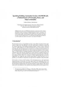
Example 2.9 We can now write more elaborated scenarios for the system of example 2.3. In this new version, the system works almost properly for about 1000 reactions: if c is true, x tends to t 9 times out of 10, otherwise it tends to 0. During this phase, the gain for the filters (a) randomly changes each 30 to 40 reactions. At last, the system breaks down and x quickly tends to 0. system foo(c: bool; t: real) returns (x: real) = within(x, -100.0, 100.0) fby local a: real in let gen gain() : trace = loop { within(a, 0.8, 0.9) fby loop[30,40] (a = pre a) } in as long as ( gen gain(), loop~1000:100 { (c and fof(x, a, t)) weight 9 | fof(x, a, 0.0) } } fby loop fof(x, 0.7, 0.0) The following timing diagram shows an execution of this program where the input t is constant (150), and the command c toggles each about 50 steps. 160 140 120 100 80 60 40 20 0

_c _t _x

0

200

400

600 steps

9

800

1000

1200

Raymond, Roux, Jahier

3

Operational semantics

3.1

Abstract syntax

For the sake of simplicity, the semantics is given on the flat language (user defined macros are inlined). We use the following abstract syntax, where the intuitive meaning of each construct is given as a comment: | |

(constraint)

| ε

(empty behavior)

| t\ε

(empty filter)

(ω ,ω ) t (priority loop) | tk c s (random loop) | ni=1 ti (priority) | |ni=1 ti /wi (choice) | ∗

x

| t·t

(sequence)

x

(raise) | [t ,→ t0 ] (catch) &ni=1 ti (parallel)

,→

t ::= c

This abstract syntax slightly differs from the concrete one on the following points: •

the empty behavior (ε) and the empty behavior filter (t\ε) are internal constructs that will ease the definition of the semantics,

•

random loops are normalized by making explicit their weight functions: · the stop function ωs takes the number of iteration already performed and returns the relative weight of the “stop” choice, · the continue function ωc takes the number of iteration already performed and returns the relative weight of the “continue” choice. These functions are completely determined by the loop profile in the concrete program (interval or average, together with the corresponding static arguments). See §4.2 for a precise definition of these weight functions.

•

the number of already performed iterations (k) is syntactically attached to the loop; this is convenient to define the semantics in terms of rewriting (in the initial program, this number is obviously set to 0).

Definition 3.1 T denotes the set of trace expressions, and C the set of constraints. 3.2

The execution environment

The execution takes place within an environment which stores the variable values (inputs and memories). Constraint resolution, weight evaluation and random selection are also performed by the environment. We keep this environment abstract. As a matter of fact, resolution capabilities and (pseudo)random generation may vary form one implementation to another, and they are not part of the reference semantics. The semantics is given in term of constraints generator. In order to generate constraints, the environment should provide the following procedures: Satisfiability. The predicate e |= c is true iff the constraint c is satisfiable in the environment e. Priority sort. Executing choices first requires to evaluate the weights in the environment. This is possible because weights may dynamically depends on uncontrollable variables (memories, inputs), but not on controllable variables (outputs, locals). Some weights may be evaluated to 0, in which case the corresponding choice is forbidden. Then a random selection is made, according to the actual weights, to determine a total order between the choices. 10

Raymond, Roux, Jahier

For instance, consider the following list of pairs (trace/weight), where x and y are uncontrollable variables: (t1 /x + y), (t2 /1), (t3 /y), (t4 /2) In a environment where x = 3 and y = 0, weights are evaluated to: (t1 /3), (t2 /1), (t3 /0), (t4 /2) The choice t3 is erased, and the remaining choices are randomly sorted according to their weights. The resulting (total) order may be: •

t1 , t2 , t4 with a probability 3/6 × 1/3 = 1/6

•

t1 , t4 , t2 with a probability 3/6 × 2/3 = 1/3

•

t4 , t1 , t2 with a probability 2/6 × 3/4 = 1/4

•

etc.

All these treatments are “hidden” within the function Sorte which takes a list of pairs (choice/weights) and returns an ordered choices list. 3.3

The step function

,→

An execution step is performed by the function Step(e, t), taking an environment e and a trace expression t. It returns an action which is either: c • a transition →n, which means that t produces a satisfiable constraint c and rewrite itself in the (next) trace n, x • a termination , where x is a termination flag which is either ε (normal termination), δ (deadlock) or some user-defined exception. Definition 3.2 A denotes the set of actions, and X denotes the set of termination flags. 3.4

The recursive step function

The run function is defined via a recursive function Se (t, g, s) where the parameters g and s are continuation functions returning actions. • g : C × T 7→ A is the goto function, defining how a local transition should be treated according to the calling context. • s : X 7→ A is the stop function, defining how a local termination should be treated according to the calling context. At the top-level, Se is called with the trivial continuations: x

,→

c

Step(e, t) = Se (t, g, s) with g(c, v) = →v and s(x) =

Basic traces. The empty behavior raises the termination flag in the current context. A raise statement terminates with the corresponding flag. At last, a constraint generates a goto or raises a deadlock, depending on its satisfiability. Se (ε, g, s) = s(ε) ,→

x

Se ( , g, s) = s(x) Se (c, g, s) = if e |= c then g(c, ε) else s(δ) 11

Raymond, Roux, Jahier

Sequence. The rule is straightforward: Se (t · t0 , g, s) = Se (t, g 0 , s0 ) where: 0 0 g (c, n) = g(c, n · t ) s0 (x) = if x = ε then Se (t0 , g, s) else s(x) Priority choice. We only give the definition of the binary choice, since the operator is right-associative. This rule formalizes the reactivity principle: all possibilities in t must have deadlock before t0 is taken into account. δ

,→

Se (t  t0 , g, s) = if r 6=

then r else Se (t0 , g, s) where r = Se (t, g, s)

Empty filter and priority loop. The empty filter intercepts the termination of t and replaces it by a deadlock: Se (t \ ε, g, s) = Se (t, g, s0 ) where s0 (x) = if x = ε then s(δ) else s(x) The semantics of the loop is then defined according to the equivalence: t∗ ⇔ (t \ ε) · t∗  ε Catch. This case covers the operators try (z = δ) and catch (z is an exception): z

Se ([t ,→ t0 ], g, s) = Se (t, g 0 , s0 )

where:

z

g 0 (c, n) = g(c, [n ,→ t0 ]) s0 (x) = if x = z then Se (t0 , g, s) else s(x) Parallel composition. We only give the definition of the binary case, since the operator is right-associative. Se (t & t0 , g, s) = Se (t, g 0 , s0 ) where: 0 s (x) = if x = ε then Se (t0 , g, s) else s(x) g 0 (c, n) = Se (t0 , g 00 , s00 ) s00 (x) = if x = ε then g(c, n) else s(x) g 00 (c0 , n0 ) = g(c ∧ c0 , n & n0 ) Weighted choice. The evaluation of the weights, and the (random) total ordering of the branches, are both performed by the function Sorte (cf. §3.2). if Sorte (ti /wi ) = ∅: Se (|ni=1 ti /wi , g, s) = s(δ) otherwise: Se (|ni=1 ti /wi , g, s) = Se ( Sorte (t1 /w1 , · · · , tn /wn ), g, s) Random loop. The semantics is defined according to the equivalence: (ωc ,ωs )

ti 3.5

⇔

(ω ,ωs )

(t \ ε) · ti+1c

/ωc (i) | ε/ωs (i)

A complete execution

Solving a constraint. The main role of the environment is to store the values of uncontrollable variable: it is a pair of stores “(past values, input values)”. For such an environment e = (ρ, ι), and a satisfiable constraint c, we suppose given a procedure able to produce a particular solution of c: Solveρ,ι (c) = γ (where γ is a store of controllable variables). We keep this Solve function abstract, since it may vary from one implementation to another (see §4). Execution algorithm. A complete run is defined according to: 12

Raymond, Roux, Jahier

a given sequence of input stores ι0 , ι1 , · · · , ιn , an initial (main) trace t0 , • an initial previous store (values of pre variables) ρ0 It produces a sequence of (controllable variables) stores γ1 , γ2 , ..., γk , where k ≤ n. For defining this output sequence, we use intermediate sequences of traces (t1 , · · · , tk+1 ), previous stores (ρ1 , · · · , ρk ), environments (e0 , · · · , ek ), and constraints (c0 , · · · , ck ). The relation between those sequences are listed below, for all step j = 0 · · · k: • the current environment is made of previous and input values: ej = (ρj , ιj ) cj • the current trace makes a transition: ej : tj →tj+1 • a solution of the constraint is elected: γj = Solvee (cj ) j • the previous store for the next step is the union of current inputs/outputs: ρj+1 = (ιj ⊕ γj ) At the end, we have: • either k = n, which means that the execution has run to completion, x • or (ρk+1 , ιk+1 ) : tk+1 which means that it has been aborted. •

,→

•

4

Implementation

A prototype has been developed, which implements the operational semantics presented in the previous section. This tool can: • interpret/simulate Lutin programs in a file-to-file (or pipe-to-pipe) manner. This tool serves for simulation/prototyping: several Lutin simulation sessions can be combined with other reactive process in order to animate a complex system. • compile Lutin programs into the internal format of the testing tool Lurette. This format, called Lucky, is based on flat, explicit automata [12]. In this case, Lutin serves as a high level language for designing test scenarios. 4.1

Notes on constraint solvers

The core semantics only defines how constraints are generated, not how they are solved. This choice is motivated by the fact that there is no “ideal” solver. A required characteristic of such a solver is that it must provide a constructive, complete decision procedure: methods that can fail and/or that are not able to exhibit a particular solution are clearly not suitable. Basically, a constraint solver should provide: • a syntactic analyzer for checking if the constraints are supported by the solver (e.g. linear arithmetics); this is necessary because the language syntax allows to write arbitrary constraints, • a decision procedure for the class of constraints accepted by the checker, • a precise definition of the election procedure which selects a particular solution (e.g. in terms of fairness). Even with those restriction, there is no obvious best solver: • it may be efficient but limited in terms of capabilities, • it may be powerful, but likely to be very costly in terms of time and memory. 13

Raymond, Roux, Jahier

The idea is that the user should choose between several solvers (or several options of a same solver) the one which best fits his needs. Actually, we use the solver that have been developed for the testing tool Lurette [13,14]. This solver is quite powerful, since it covers Boolean algebra and linear arithmetics. Concretely, constraints are solved by building a canonical representation which mixes Binary Decision Diagrams and convex polyhedra. Because it is very powerful, this method is also costly. However the solver benefits from several years of experimentation and optimizations (partitioning, switch form polyhedra to intervals whenever it is possible). The election of a particular solution is also quite sophisticated: • The basic rule is to ensure some fairness between the solutions. This is achieved by simulating a uniform choice among the solutions domain. Since uniform selection within a polyhedron is a complex problem, several options are available ranging from a simple, rough approximation to a very accurate, and thus costly one. • The solver can also be parameterized to select some class of interesting solutions (e.g. limit values corresponding to the polyhedra vertices).

4.2

Notes on predefined loop profiles

In the operational semantics, loops with iteration profile are translated into binary weighted choices. Those weights are dynamic: they depend on the number of (already) performed iterations k. Interval loops. For the “interval” profile, those weights functions are formally defined, and thus, they could take place in the reference semantics of the language. For a given pair of integer (min, max), such that 0 ≤ min ≤ max, and a number k of already performed iterations, we have: • if k < min then ωs (k) = 0 and ωc (k) = 1 (loop is mandatory), • if k ≥ max then ωs (k) = 1 and ωc (k) = 0 (stop is mandatory), • if min ≤ k < max then ωs (k) = 1 and ωc (k) = 1 + max − k Average loops. There is no obvious solution for implementing the “average” profile in terms of weights. A more or less sophisticated (and accurate) solution should be retained, depending on the expected precision. In the actual implementation, for an average value av and a standard variation sv, we use a relatively simple approximation: • First of all, the underlying discrete repartition law is approximated by a continuous (Gaussian) law. As a consequence, the result will not be accurate if av is too close to 0, and/or if st is too big comparing to av. Concretely we must have 10 < 4 ∗ sv < av. • The Gaussian repartition, for which it is well known that there is no algebraic form, is itself approximated by using an interpolation table (512 samples with a fixed precision of 4 digits). 14

Raymond, Roux, Jahier

5

Conclusion

We propose a language for describing constrained-random reactive system. Its first purpose is to describe test scenarios, but it may also be useful for prototyping and simulation. We have developed a compiler/interpreter which strictly implements the operational semantics presented here. Thanks to this tool, the language is integrated into the framework of the tool Lurette, where it is used to describe test scenarios. Further works concerns the integration of the language within a more general prototyping framework. Other works concern the evolution of the language. We plan to introduce a notion of signal (i.e. event), which is useful for describing values that are not always available (this is related to the notion of clocks in synchronous languages). We also plan to allow the definition of (mutually) tail-recursive traces. Concretely, that means that a new programming style would be allowed, based on explicit concurrent, hierarchic automata.

References [1] Raymond, P., Roux, Y.: Describing non-deterministic reactive systems by means of regular expressions. In: First Workshop on Synchronous Languages, Applications and Programming, SLAP’02, Grenoble (2002) [2] Halbwachs, N.: Synchronous programming of reactive systems. Kluwer Academic Pub. (1993) [3] Berry, G., Gonthier, G.: The Esterel synchronous programming language: Design, semantics, implementation. Science of Computer Programming 19 (1992) 87–152 [4] Halbwachs, N., Caspi, P., Raymond, P., Pilaud, D.: The synchronous dataflow programming language Lustre. Proceedings of the IEEE 79 (1991) 1305–1320 [5] Lynch, N.A., Tuttle, M.R.: An introduction to Input/Output automata. CWI-Quarterly 2 (1989) 219–246 [6] Wu, S.H., Smolka, S.A., Stark, E.W.: Composition and behaviors of probabilistic I/O automata. Theoretical Computer Science 176 (1997) 1–38 [7] Jonsson, B., Larsen, K., Yi, W.: Probabilistic extensions of process algebras (2001) [8] Bernardo, M., Donatiello, L., Ciancarini, P.: Stochastic process algebra: From an algebraic formalism to an architectural description language. Lecture Notes in Computer Science 2459 (2002) [9] Saraswat, V.A., ed.: Concurrent Constraint Programming. MIT Press (1993) [10] Saraswat, V.A., Jagadeesan, R., Gupta, V.: Foundations of timed concurrent constraint programming. In: LICS. (1994) 71–80 [11] Nielsen, M., Palamidessi, C., D.Valencia, F.: Temporal concurrent constraint programming: Denotation, logic and applications. Nord. J. Comput 9 (2002) 145–188 [12] Raymond, P., Jahier, E., Roux, Y.: Describing and executing random reactive systems. In: SEFM 2006, 4th IEEE International Conference on Software Engineering and Formal Methods, Pune, India (2006) [13] Raymond, P., Weber, D., Nicollin, X., Halbwachs, N.: Automatic testing of reactive systems. In: 19th IEEE Real-Time Systems Symposium, Madrid, Spain (1998) [14] Jahier, E., Raymond, P., Baufreton, P.: Case studies with lurette v2. In: Software Tools for Technology Transfer. Volume 8. (2006) 517–530

15