Spectral Interpretation Based on Multisensor Fusion for Urban Mapping

Spectral Interpretation Based on Multisensor Fusion for Urban Mapping Be´ata Csath´o

Toni Schenk and Suyoung Seo

Byrd Polar Research Center The Ohio State University 1090 Carmack Rd., Columbus, OH 43210 Email: [email protected]

CEEGS 2070 Neil Ave., The Ohio State University Columbus, OH 43210 Email: [[email protected], [email protected]]

Abstract— This paper is concerned with fusing aerial imagery, LIDAR point clouds, and hyperspectral imagery for the purpose of automated urban mapping. Instead of performing traditional supervised and unsupervised classification of hyperspectral data we propose a region growing approach from seed pixels that originate from fusing LIDAR and aerial imagery. This requires a thorough alignment of all sensors involved—a problem that is solved with sensor invariant features. The common system is the geodetic reference frame in which the LIDAR points are computed. The alignment results in transformations from sensor space to object space and back, avoiding resampling the sensor data. After describing the major aspects, an example demonstrates the feasibility of the proposed fusion approach.

I. INTRODUCTION

By combining sensors that use different physical principles and record different properties of the object space, complementary and redundant information becomes available. If merged properly, multisensor data may lead to a more stable and consistent scene description. The cardinal question of future research is how to exploit the potential these different data sources offer in order to tackle object recognition more effectively. Ideally, proven concepts and methods in remote sensing, digital photogrammetry and computer vision should be combined in a synergistic fashion. In this paper, we propose a unified framework for object recognition and multisensor data fusion for reconstructing urban scenes. Photogrammetry is the traditional method of surface reconstruction such as the generation of DTMs. Recently, LIDAR emerged as a new technology for rapidly capturing data of physical surfaces. The high accuracy and automation potential enables a quick delivery of DEMs/DTMs derived from the raw laser data for urban areas. Multispectral and even multisensor data can provide further clues about surface properties, such as composition, roughness and slope. The increasing spatial resolution and accuracy, together with the rich information content of hyperspectral image data opens new avenues for automating surface reconstruction and object recognition of urban environments. Most researchers use proven processing techniques, such as image enhancement, computation of spectral indices, spectral unmixing and patternrecognition, for extracting information from hyperspectral imagery (for example [8] and [5]). The interpretation of the

data set usually ends with classifying the pixels into different cover types, or with the determination of the percentage of cover types by using subpixel estimation techniques. To increase the reliability and robustness of classification many researchers favor supervised techniques. These techniques are comparable to early vision processes and they work efficiently on data sets with low spectral dimensions, such as Landsat or SPOT satellite imagery. However, when increasing the number of channels, two problems arise: the classification time increases significantly and there may be not enough training pixels in small classes for reliably estimating the class statistics. Band reduction techniques and multistage algorithms are recommended to overcome these limitations ([4], [7] and [2]). Unfortunately, the use of supervised classification reduces the degree of automation. Also the interactive training is tedious, time consuming, and subjective. Moreover, the band reduction techniques usually rely on the statistics of the whole image, therefore spectral signatures caused by small objects are not well preserved. spectra This paper suggest to use the explicit surface description obtained from LIDAR data and aerial photography by segmentation and grouping processes to guide the segmentation of the hyperspectral data set. Photogrammetry, LIDAR mapping and hyperspectral imaging deliver complementary surface information. Thus it makes sense to combine data from the different sensors to arrive at a more robust and complete surface reconstruction. II. MAPPING URBAN SCENES BY SPECTRAL IMAGING

The majority of multi- and hyperspectral sensors (also called imaging spectrometers) sample the reflective portion of the EM spectrum that extends from the visible region (0.4-0.7 µm) through the near-infrared (about 2.5 µm). Spectral reflectivity of the ground materials can be inferred from the measured signal. Hyperspectral sensors measure the spectral irradiance at the sensor in many, often in hundreds, of narrow, contiguous spectral bands. Multispectral sensors have fewer discrete, wide spectral bands. The scanning principle of spectral imaging sensors includes pushbroom (linescanner), or whiskbroom (rotating mirror, similar to laser scanning).

Spectral imaging dates back to the first Landsat satellite program, which started in 1972. Its synoptic, repeat coverage, and the spectral information made the Landsat and other satellite imagery ideal for earth science applications and for mapping land cover changes. The low spectral and spatial resolution of these images did not allow detailed mapping of urban areas, however. Hyperspectral sensors depict important details of the EM spectrum, such as the shape of narrow absorption bands allowing delineation and in some cases even identification of surface materials. This capability taken together with the few meter spatial resolution will make airborne hyperspectral sensors suitable for providing surface composition information to urban mapping. The traditional procedure to map surface materials from hyperspectral imagery starts with dimensionality reduction followed by supervised classification. Landgrebe [5] reduced the number of bands by analyzing the spectral characteristics and separability of the classes defined by the training samples. The classification was performed by a spectral and spatial quadratic maximum likelihood classifier. McKeown et al., [8] simply averaged the reflectivity of neighboring spectral bands prior to applying a spectral maximum likelihood classification. Both authors pointed out the importance of careful and tedious training and the large number of subclasses needed to describe the variety of different roof and road materials. The spatial resolution of most hyperspectral data sets is a few meters and therefore they may not able to depict the details of small urban structures. To deal with the large number of mixed pixels over object boundaries, Roessner et al., [10] developed a technique that combines the advantages of classification with linear spectral unmixing. Unlike these supervised methods the Gibbs-based algorithm developed by Rand and Keenan [9] is suitable for automation. This algorithm, using spectral angle as disparity metric and a random initialization, partitioned moderate-high scene complexity test images into homogeneous, structured regions of different urban and natural objects. III. PROPOSED FUSION SCHEME Over the years, several fusion models and archtictures for fusion system have been introduced. The Joint Directors of laboratories (JDL) Data Fusion Working Group created a data fusion process model and undertook efforts to unify terminology. An excellent overview of this model and its variants is presented in [3]. Other efforts to categorize fusion include attempts to break it down into the three levels of data fusion, information fusion, and decison fusion. In contrast to existing data fusion models, we propose a clear separation between fusion processes (functionality) and fusion tasks (applications). The motivation for this distinction stems from the observation that fusion tasks such as sensor alignment, surface reconstruction, object extraction and identification, are independently solved by employing the same fusion functionality. Fig. 1 depicts the flowchart of the proposed multisensor fusion framework. The processes on the left side are devoted to establishment of a common reference frame for the sensory

input data. The result is a unique transformation between the sensor systems and the reference frame. L

A

H

L’

A’

H’

sensor-invariant feature extraction

geometric & semantic feature extraction

feature correspondence

feature-based fusion

common reference frame

reconstructed 3D surface

Fig. 1.

Schematic diagram of a feature based fusion system.

The establishment of a common reference frame is an absolute prerequisite. We solve this alignment problem by utilizing sensor-invariant features. Such features correspond to the same object space phenomena, for example to breaklines and surface patches. Matched sensor invariant features from the three different data sets lend themselves to establishing a common reference frame. Feature-level fusion of the LIDAR and the aerial imagery is then performed with sensor specific features that are related to surface characteristics. Details of the proposed approached are described in [11]. We have shown that the synergism between these features resulting in a richer and more abstract surface description. This explicit surface description obtained from LIDAR data and aerial photography by segmentation and grouping processes is used to guide the segmentation of the hyperspectral data set. First seed pixels are selected in object space based on the surface description derived from the LIDAR data and the aerial photography. A region growing algorithm is then applied to find uniform regions within the hyperspectral data set. Results from the hyperspectral segmentation are fused with features extracted from the aerial imagery and the LIDAR data set to improve the surface description. The fusion process is embedded in an inference scheme. For example, unlike in traditional classification, labels of landcover types are not assigned to each pixel, but to the regions detected by region growing. To make the labeling process more robust additional (non-spectral) information, for example elevation data and edges extracted and grouped from aerial imagery are also considered. During the inference process, hypotheses are formed about objects and their interrelationships. An important aspect is the verification of these hypotheses, for example by examining interrelationships among objects or by testing alternative hypothesis. At this stage it may be necessary to go back to the original data with expectations what to look for. As an example, a new segmentation of the hyperspectral scene may be started with modified parameters that take into

account the current knowledge about the scene. IV. STUDY AREA, DATA AND PREPROCESSING OF HYPERSPECTRAL IMAGERY

We demonstrate the feasibility of the proposed fusion approach by using data from the Ocean City test site. Aerial photography, laser scanning data, and multispectral imagery were collected on April 25 and 30, 1997. Details about the data acquisition and processing are described in [1]. AVIRIS hyperspectral imagery were acquired on November 5, 1998, when the AVIRIS system was first deployed on a relatively low altitude platform to collect high quality, high spatial resolution imagery. The flight altitude of 4000 meter resulted in a pixel size of about 3.8 meter. The AVIRIS sensor is a whiskbroom imaging spectrometer using an oscillating mirror to cover a 30 degree field of view at a rate of 12 Hz. Upwelling radiance is measured through 224 contiguous spectral channels at 10 nm interval across the visible and nearinfrared spectrum. The processing of the AVIRIS data at JPL included the rectification of raw images by estimating the exterior orientation of each pixel from the scanner geometry and GPS/INS data. To convert the radiance to surface reflectance we applied empirical line calibration using field reflectance data collected during the overflight. The data set provided by hyperspectral sensors is a set of coregistered imagery, one image for each spectral band. A convenient way to visualize the data set is to use a data cube, whose face is a function of spatial coordinates and the depth is a function of the spectral band or wavelength. That is a spectrum, characterizing the materials within the pixel is provided for each image pixel. The organization and the rich information content of the data set is illustrated in Fig. 2 and Fig. 3 .

Fig. 2. AVIRIS image cube from a sub-scene of the Ocean City imagery. Cover plane is a simulated color infrared image from bands 15 (0.51 µm), 25 (0.61 µm)and 45 (0.78 µm). Coloring on sides shows reflectance (warm colors=high reflectance).

Fig. 3.

Spectra of common urban materials from the AVIRIS scene.

V. FUSION OF AERIAL PHOTOGRAPHS, LIDAR AND HYPERSPECTRAL DATA SETS

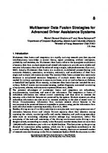
In this section we briefly explain the major processing steps and demonstrate the feasibility of the proposed approach to reconstruct surfaces of the Ocean City scene. A. Establishment of A Common Reference Frame The first step in our fusion approach involves the establishment of a common reference frame for the sensory input data. This entails a geometric transformation, accomplished with features extracted from the sensors that are also known in object space. Hence, the sensors to be aligned must partially respond to the same phenomena in object. Such features are called sensor invariant in this paper. First we oriented the aerial photographs with respect to the laser point cloud by using sensor invariant features, including straight lines and surface patches ([11]). The AVIRIS scene distributed by JPL was registered to a flat earth. While this may suffice for satellite imagery with relatively coarse ground resolution, it does not meet the requirements of large-scale, urban fusion applications. To derive the transformation, the geometry of the whiskbroom scanner is emulated by that of a line scanner. The advantage of this approach is that existing solutions for orienting line scanners can be employed. As shown in [6], every line of a line scanner can independently be oriented by using linear features. In contrast to the traditional direct solution that depends entirely on GPS/INS data, the indirect solution uses the navigation data only as approximations. Linear features in object space are slightly distorted in the line image due to changes in the exterior orientation of every line. For example, a straight line appears jagged or curved (Fig. 4). The basic principle of the indirect line sensor orientation is to change the orientation parameters of every line by minimizing the shape differences between image and object space features. B. Surface Reconstruction from Multiple Sensors A small sub-area of the southern part of Ocean City is selected to demonstrate the surface reconstruction (Fig. 5(a,b)). It contains a large building with a complex roof structure,

Fig. 4. Salient features used for registration of AVIRIS scene. Linear feaures are shown on the aerial imagery in Fig. 4(a). Corresponding features are extracted from the AVIRIS scene by region growing (Fig. 4(b). Seed pixels are selected within regions of low variance and the boundaries are refined by dilation and skeleton definition.

surrounded by parking lots, garden, trees and foundation plants that are in close proximity to the building. The result of fusing aerial images and LIDAR data is shown in Fig. 5(c). The regions 0 to 18 are planar surface patches obtained from the perceptual organization of the laser points. The straight edges are either from the stereopair or from intersecting adjacent planar surface patches. The AVIRIS scene reveals a variety of man-made materials (roof tops, roads, boardwalks, etc.) with very different spectral shapes and absorption bands (Fig. 3 ). The large number of different spectral classes taken together with the small total area of some object and the presence of mixed pixels would pose a difficult problem for unsupervised classification. Therefore we apply a simple region growing algorithm to segment the AVIRIS scene into spectrally homogeneous regions. The spectral similarity is measured by a spectral angular metric (often called SAM). The SAM metric is a good indicator of differences in spectral shape, while insensitive to brightness differences. To guide the region growing process, the surface patches obtained by fusing the aerial images and lidar data (Fig. 5(c) are back-projected to the AVIRIS scene using the geometric transformation established between the different data sets in Section V.A. Seed pixels are selected within the backprojected patches (Fig. 5(d,e)). The regions of the segmented hyperspectral scene in Fig. 5(f) correspond to the different regions of the scene as it is verified by visual inspection of the aerial photograph and by comparing it with the result of the linear spectral unmixing of the AVIRIS subscene (Fig. 5(g,h)). Finally, Fig. 5(i) shows the result of the fusion process. The segmented surface (Fig. 5(c)) is now augmented with surface property information, stemming from the region growing process of the hyperspectral data. VI. CONCLUSIONS AND FUTURE WORK We have presented a new approach for multisensor data fusion that is particularly suited for urban mapping, using the combination of aerial and satellite imagery, LIDAR point clouds, and hyperspectral imagery. A key element is the sensor

alignment with rigorous transformations from sensor systems to object space and back. This offers the advantage of working with the raw sensory data, rather than with resampled data sets that may suffer a potential loss in geometric and radiometric resolution. In order to avoid time consuming training sessions for segmenting hyperspectral data we propose a region growing approach that starts with seed regions obtained from the perceptual organization of the laser point cloud and the fusion of aerial imagery. This approach greatly facilitates automation, an important objective of urban mapping. The region growing approach takes all spectral bands into account and can be driven by application know-how or scene knowledge gained during the fusion process. The precise registration of hyperspectral data is still quite problematic, especially in the case of whiskbroom sensors. We are currently investigating improved sensor models. Another area that needs more attention is higher level reasoning to better guide the the fusion processes. Acknowledgement The authors would like to thank NASA JPL, NASA WFF and NGS for data collection and processing, Impyeong Lee for sharing results of perceptual organization of laser surfaces, Grady Tuell for providing help in processing AVIRIS data, and Tzu-lung Sun for his help in segmenting hyperspectral data. References [1] Csath´o, B., W. Krabill, J. Lucas and T. Schenk, "A multisensor data set of an urban and coastal scene," ISPRS Intern. Archives, vol. 32, part 3/2, pp. 15–21, 1998. [2] Green, A. A., M. Berman, P. Switzer and M. D. Craig, "A transformation for ordering multispectral data in terms of image quality with implications for noise removal," IEEE Trans. Geosci. Remote Sensing, vol. 26, pp. 65– 74, 1988. [3] Hall, D. and J. Llinas (1997). An Introduction to Multisensor Data Fusion. Proc. IEEE, 85(1), pp.6-23. [4] Jia, X., and J. A. Richards, "Efficient maximum likelihood classification for imaging spectrometer data sets, " IEEE Trans. Geosci.Remote Sensing, vol. 32, pp. 274–281, 1994. [5] Landgrebe, D., "Hyperspectral image data analysis", IEEE Signal Processing Magazine, pp. 17–28, January 2002. [6] Lee, Y. Pose estimation of line cameras using linear features. PhD dissertation, Department of Civil and Environmental Engineering and Geodetic Science, OSU, 162 p., 2002. [7] Lee, C. and D. A. Landgrebe, "Fast likelihood classification," IEEE Trans. Geosci. Remote Sensing, vol. 29, pp. 509–517, 1991. [8] McKeown, D. M., S. D. Cochran, S. J. Ford, C. McGlone, J. A. Shufelt and D. A. Yosum, "Fusion of HYDICE hyperspectral data with panchromatic imagery for cartographic feature extraction," IEEE Trans. Geosci. Remote Sensing, vol. 37, pp. 1261–1277, 1999. [9] Rand, R. S. and D. M. Keenan, "A spectral mixture process conditioned by Gibbs-based partitioning," IEEE Trans. Geosci. Remote Sensing, vol. 39, pp. 1421–1434, 2001. [10] Roessner, S., K. Segl, U. Heiden, and H. Kaufmann, "Automated differentiation of urban surfaces based on airborne hyperspectral imagery," IEEE Trans. Geosci. Remote Sensing, Vol. 39, No. 7, pp. 1525–1532, 2001. [11] Schenk, T. and B. Csath´o, "Fusion of LIDAR data and aerial imagery for a more complete surface description," ISPRS Intern. Archives, Vol. 34, Part 3A, 310–317, 2002.

(a)

(b)

(c)

(d)

(e)

(f)

(g)

(h)

(i)

Fig. 5: Results of fusing hyperspectral imagery with aerial photograph photographs and lidar data. Fig. 5(a) shows the test site of Ocean City on a color composit e of three bands from the AVIRIS image and (b) depicts the subarea that was used to demonstr ate the detailed surface reconstruction indicate d by white box in a). In Fig. 5(c) the surface reconstructed from aerial images and LIDAR data is shown from [11]. Fig. 5(d) shows the AVIRIS color composit e of the subarea. Fig. 5(e) contains the result of segmentati on of AVIRIS imagery obtained by region growing. Seed pixels are selected as centroid s of the surface patches reconstructed from LIDAR and aerial photographs (see also in Fig. 5(d)). Fig. 5(f) shows the spectra of the surface material at the seed points marked in Fig. 5(d,e). Fig. 5(g,h) depicts the distribution of ’roof’ and ’vegetation ’ from spectral linear unmixing of the AVIRIS scenes by using ’roof ’, ’asphalt’ and ’vegetation ’ spectra for spectral endmembers. Fig. 5(i) summariz es the results of the surface reconstruction. The color code of the region boundaries corresponds to: black: AVIRIS; yellow and green: LIDAR and aerial imagery.