Speech Text-independent Segmentation Using an Improvement Method for Identification of Phoneme Boundaries Ricardo Sánchez Jurado, Pilar Gómez-Gil, Carlos A. Reyes García Instituto Nacional de Astrofísica, Óptica y Electrónica
[email protected],
[email protected],
[email protected]
Abstract The determination of right boundaries during phoneme segmentation of a speech signal is an important part in the process of automatic speech recognition. However, when no information is provided about the meaning of the signal, this segmentation process becomes very difficult. Currently, most of the methods used to detect boundaries of phonemes are based in the identification of variations in distances calculated over a set of features, which are obtained from segments of the signal. Here we present a modification of a previous work, that is based on a different calculation of the distances and a modification in the selection of a boundary. The proposed modification showed to improve the correct segmentation percentage when compared with the previous work, tested in Spanish and English corpus. The improved method obtained 82.59% of correct segmentation over Spanish data, and 80.28% over English data. In addition, the proposed method obtained at average an oversegmentation of 0%.
1. Introduction Automatic speech recognition is an area of pattern recognition that has obtained important advances lately. A main component of speech recognition is segmentation, which is the process of dividing a speech signal into small units, in a fully automatic way. Segmentation may be based in phonemes, syllables or words. Phoneme segmentation has an important advantage over other types of segmentation, because few tokens are generated to be used in the next recognition step, which is phoneme transcription. Determination of the right boundaries in a signal where each phoneme starts and finishes is a difficult task if the only information provided to the system is the signal. In the last years, several works related to speech text-independent segmentation (for example [2,3,4,9]) have look for ways to improve the performance of this task. In this article we present
some improvements over the work developed by Huerta [3]. Such improvements were obtained by modifications of the calculation of distances and boundary selection (see figure 1). The performance of the proposed modifications is evaluated with both English and Spanish corpus.
Figure 1. Segmentation process for text independent speech recognition This paper is organized as follows: section 2 briefly introduces the process for text-independent speech segmentation. Section 3 shows the details for the codification method used in this research; section 4 describes metrics used for distance calculations; section 5 shows the method to select candidates for boundaries; section 6 presents the results obtained. Finally, section 7 comments on conclusions and future work.
2. Text-independent segmentation process This type of speech segmentation takes place without any prior knowledge of the signal being processed. Segmentation starts with a codification of the signal to reduce the amount of information and to get features. Some well known codification methods are MFCC (Mel-frequency cepstral coefficient) and Melbanks (Mel Filter Banks). Huerta [3] and Esposito [4] reported that Melbanks obtained better results than MFCC when applied to speech signals, partly because Melbanks gets a small number of features of the original signal for each frame. After coding the signal, the produced features are used to measure variations among frames. A set of distance
To be published at the proceedings of the 2009 International Conference on Electrical, Communications, and Computers, CONIELECOMP 2009, Cholula, México. IEEE Computer Society Press. Feb. 2009
values is obtained and analyzed to identify the place where a transition among phonemes exists. Such positions are known as phoneme boundaries. Two contiguous phoneme boundaries correspond to initial and final values of a phoneme.
one. Membership values are in [0,1]. Using fuzzy representation, there are 3 values for each entry at matrix C.
3. Signal codification 3.1 Melbanks Melbanks resembles the way in that human listens. It is known that human ear may perceive sounds in a frequency range from 20 to 20,000 Hz [5], and that variations of frequencies are perceived following a logarithmic scale. Some researchers have concluded that the hearing process is based on frequency decomposition of the listening signal using something similar to a bank filter [1]. Melbanks uses filters that overlap and are centered in frequencies located in a non-linear Mel scale, as proposed by Stevens y Volkman [6]. Figure 2 shows this scale. The number of filters, which can have a triangular or Hamming shape, depends on the number of features. Codification takes place as follows: first, the signal is divided in segments of 20 ms. with an overlap of 10 ms. Second, each segment enters to the filters, where each sub-band (S) is analyzed calculating the “log energy” entropy:
E (S ) = ∑ log( S i ) 2
Figura 2. Mel scale.
Figure 3. Getting n features for one signal frame
(1)
i
which is used as the representing features of the frame. For the experiments reported here, 8 and 12 filters were used, getting an nxm matrix C, where n is the number of signal frames and m is the number of filters. The codification process is shown at figure 3 for one frame. Figure 4. Fuzzy sets used in this work
3.2 Fuzzy Features. Due to the fact that transactions among frames may be not clearly defined, Huerta [3] proposed to assign a fuzzy value to each feature using fuzzy sets. When features of each frame are compared using similar numerical values (real values), fuzzy values allow the generation of prominent distances using the distance metrics presented at section 4. In this work three fuzzy sets were used: High, medium and low, represented by triangular functions overlapped by 50% (figure 4). A fuzzy space for these sets is defined for each sub-band, calculating the maximum and minimum value for each
4. Distances among frames. From the calculation of distances among features of frames, it is possible to generate prominent values that show transitions among phonemes identifying a phoneme boundary. Vector distances can be calculated using different formulas, as Manhattan’s, Euclidian’s, Chevishev’s or others. Euclidian’s (equation 2) and a modification of Chebyshev’s distance (equation 3) are used in this research. Such modification consists on squaring the obtained distance value, as shown in equation 3.
To be published at the proceedings of the 2009 International Conference on Electrical, Communications, and Computers, CONIELECOMP 2009, Cholula, México. IEEE Computer Society Press. Feb. 2009
1
n
d ( X , Y ) = (∑ ( xi − yi) 2 ) 2
(2)
i =1
d ( X , Y ) = max i =1... n {( xi − y i ) 2 }
(3)
The number of contiguous frames involved in the calculation of this metric and the use of fuzzy values are other important issues to be considered. If two contiguous frames are used, a good resolution, that is, transactions nearby can be detected, but in the other hand, it is possible that such transactions may refer to the same phoneme, generating over segmentation. We used four contiguous using the formula:
D( fm,..., fm + 3) =
m +1 m + 3
n
( Ai ,k − A j ,k ) 2 +
∑ ∑ ∑(M i = m j = m + 2 k =1
i ,k
English and Spanish corpuses were used to test the method: DIMEx100 [7] is a Spanish corpus with 6,000 phrases coming from 100 subjects, each recording 60 different phrases. They were sampling in mono mode with 16 bits at 44.1 KHz. TIMIT [8] contains 630 speakers with 8 dialects of American English. Each speaker recorded 10 sentences at 16K Hz, therefore 6,300 sentences were recorded.
(4)
− M j ,k ) 2 +
( Bi ,k − B j ,k ) 2
where {A, M, B} represent membership values for each of the n frame features. The distance used for the proposed modification to Chevyshev is calculated by: ( Ai ,k − A j ,k ) 2 , (5) D( fm,..., fm + 3) = ∑ ∑ ∑ max ( M i ,k − M j ,k ) 2 , i = m j = m + 2 k =1 B 2 ( i ,k − B j ,k ) m +1 m +3
5. Choosing candidates for boundaries After calculating distances, these are analyzed to figure out if the maximum values indicate a transaction. Distances can be seen as points in a graph (see figure 5), where local maxima are considered transactions among phonemes, that is, boundaries [3, 4]. To be considered a boundary, a local maximum must satisfy the following conditions: 1) ( Dt −1 < Dt ) y ( Dt +1 < Dt + 2 ) 2) Dt , Dt +1 > Φ
(6) (7)
where Φ is a threshold and Dt y Dt+1 are distance values calculated among contiguous frames. Index t represents the time where such value occurs. Each t increment represents 10 milliseconds. Figure 5 shows how 2 maximum points are selected to represent a candidate for a boundary.
6. Results 6.1 Data set
Figure 5. Selection of boundary candidates
n
6.2 Data for the experiments Eight sentences of 30 speakers (18 men and 12 women) were selected from DIMEx100 to test the method, giving a total of 240 sentences. The total of real phoneme boundaries in this test is 11,046. Eight sentences of 60 speakers (30 men and 30 women) were selected from TIMIT corpus, giving a total of 480 sentences. This data set contains 18,162 phoneme boundaries.
6.3 Performance evaluation The method was evaluated using the common metrics: percentage of right detections and percentage of over-segmentation. We consider a time instance detected correct if it is under ±20 mili-seconds with respect to the real phoneme boundary in the data set. Correct segmentation percentage Pc is calculated as:
Pc = 100 * (
Sc ) St
(8)
where Sc is the total of correct boundaries detected and St is the number of real boundaries. An insertion occurs where the detected phoneme boundary is not in the tolerance of ±20 milliseconds. The number of inserted point is used to calculate the
To be published at the proceedings of the 2009 International Conference on Electrical, Communications, and Computers, CONIELECOMP 2009, Cholula, México. IEEE Computer Society Press. Feb. 2009
percentage of over segmentation (also known as percentage of insertions). This is calculated as:
Pi = 100 * (
Sd ) St
(9)
Sd is the total number of detected boundaries. For an ideal case Pc =100% and Pi = 0%.
6.4 Segmentation Results Table 1 presents the results obtained by the proposed method when applied to the DIMEx100 data set. Twelve filters were used in this case. The method was applied to the 240 sentences. This and next table report the average of the percentages obtained for each sentence, as well as the best and worst cases. Table 2 presents the results for TIMIT database, where 7 filters were used. In this case 480 sentences were processed. Table 3 compares the results obtained in this work with the results obtained by Huerta [3]. Notice that for both corpuses our method obtained better results that [3]. In average, Segmentation rate in all cases was bigger than Huerta’s as well as over segmentation percentage was kept at 0%.
The obtained results show that the modification on the distance calculation and selection of candidates for boundaries improve the segmentation process in English and Spanish corpuses. The improvement in the performance over TIMIT corpus (English) is greater than over DIMEx100 (Spanish). It should be pointed out that these results are equivalent to the work reported at [4], which is one of the best results obtained currently in Spanish corpus. As future work, we propose to include in this method the use of Wavelets as a codification schema, which have proved to be an alternative to Melbanks [9]. Also the effect of noise in the proposed method requires to be studied. Table 1. Segmentation results for DIMEx100 data set Real Boundaries Total boundaries detected Correct Boundaries Incorrect Boundaries Correct segmentation
Best case in data set
0%
0%
-25%
Table 2. Segmentation results for TIMIT data set. Average over 480 sentences Real Boundaries Total boundaries detected Correct Boundaries Incorrect Boundaries Correct segmentation Pc Oversegmentation
Method Proposed Huerta’s [3]
Best case in data set
Worst case in data set
18,162
17
27
18,165
17
19
14,571
16
13
3,591
1
6
80.28%
94.12%
48.15%
0%
0%
-29.6%
Table 3. Comparative results Corpus Pc Pi DIMEx100 82.58% 0.00% TIMIT 80.28% 0.00% DIMEx100 79.89% 0.08% TIMIT 76.50% -0.08%
8. References
7. Conclusions and Future Work
Average over 240 sentences
Pc Oversegmentation
Worst case in data set
11,046
50
40
11,047
50
30
9,122
46
26
1,925
4
4
82.58%
92%
65%
[1] J. Bernal, J. Bobadilla, P. Gómez. “Reconocimiento de Voz y Fonética Acústica”. Editorial RA-MA, Madrid, España. 2000. [2] J. Adell, A. Bonafonte, J. A. Gómez, M. J. Castro. “Análisis de la Segmentación Automática de Fonemas para la Síntesis de Voz”. Universidad Politécnica de Cataluña (UPC), 2004. [3] L. D. Huerta. “Segmentación del habla con independencia de texto”. Tesis de Maestría en Ciencias Computacionales. Instituto Nacional de Astrofísica Óptica y Electrónica. Tonantzintla, Puebla, México, 2006. [4] A. Esposito, G. Aversano. “Text independent Methods for Speech Segmentation”. In: Proc. Lecture Notes in Computer Science, pp. 261-290, 2005 [5] Manfred R. Schroeder. “Computer Speech Recognition, Compression, Synthesis”. Springer series in information science Vol. 35. 1999 [6] Volkman J. Stevens S. “The relation of pitch to frequency”. American Journal of Psychology, 1940. [7] Pineda, L.A., Villaseñor-Pineda, L., Cuétara, J., Castellanos, H. & López, I. “DIMEx100: A New Phonetic and Speech corpus for Mexican Spanish”. Proceedings of the 9th Ibero-American Conference on AI, (IBERAMIA), Puebla,
To be published at the proceedings of the 2009 International Conference on Electrical, Communications, and Computers, CONIELECOMP 2009, Cholula, México. IEEE Computer Society Press. Feb. 2009
Mexico, November 22-25, 2004. Lecture Notes in Artificial Intelligence, Vol. 3315, pp. 974-983, Springer 2004. [8] Lamel L. Garofolo J. “Darpa timit acoutic-phonetic continuous speech corpus”. Technical report, U.S Departament of Commerce. 1993. [9] Analía S. Cherniz, María E. Torres, Hugo L. Rufiner, Anna Esposito. “Multiresolution analysis applied to textindependent phone segmentation”. 16th Argentine Bioengineering Congress and the 5th Conference of Clinical Engineering. IOP Publishing. Journal of Physics: Conference Series 90, 2007
To be published at the proceedings of the 2009 International Conference on Electrical, Communications, and Computers, CONIELECOMP 2009, Cholula, México. IEEE Computer Society Press. Feb. 2009