Segmentation Using an Adaptive Multi-Cost

SS symmetry Article

Accurate Dense Stereo Matching Based on Image Segmentation Using an Adaptive Multi-Cost Approach Ning Ma 1,2 , Yubo Men 1 , Chaoguang Men 1, * and Xiang Li 1 1

2

*

College of Computer Science and Technology, Harbin Engineering University, Nantong Street 145, Harbin 150001, China; [email protected] (N.M.); [email protected] (Y.M.); [email protected] (X.L.) College of Computer Science and Information Engineering, Harbin Normal University, Normal University Road 1, Harbin 150001, China Correspondence: [email protected]; Tel.: +86-451-86207610

Academic Editor: Angel Garrido Received: 23 August 2016; Accepted: 12 December 2016; Published: 21 December 2016

Abstract: This paper presents a segmentation-based stereo matching algorithm using an adaptive multi-cost approach, which is exploited for obtaining accuracy disparity maps. The main contribution is to integrate the appealing properties of multi-cost approach into the segmentation-based framework. Firstly, the reference image is segmented by using the mean-shift algorithm. Secondly, the initial disparity of each segment is estimated by an adaptive multi-cost method, which consists of a novel multi-cost function and an adaptive support window cost aggregation strategy. The multi-cost function increases the robustness of the initial raw matching costs calculation and the adaptive window reduces the matching ambiguity effectively. Thirdly, an iterative outlier suppression and disparity plane parameters fitting algorithm is designed to estimate the disparity plane parameters. Lastly, an energy function is formulated in segment domain, and the optimal plane label is approximated by belief propagation. The experimental results with the Middlebury stereo datasets, along with synthesized and real-world stereo images, demonstrate the effectiveness of the proposed approach. Keywords: stereo matching; multi-cost; image segmentation; disparity plane fitting; belief propagation

1. Introduction Stereo matching is one of the most widely studied topics in computer vision. The aim of stereo matching is to estimate the disparity map between two or more images taken from different views for the same scene, and then extract the 3D information from the estimated disparity [1]. Intuitively, the disparity represents the displacement vectors between corresponding pixels that horizontally shift from the left image to the right image [2]. Stereo matching serves an important role in a wide range of applications, such as robot navigation, virtual reality, photogrammetry, people/object tracking, autonomous vehicles, and free-view video [3]. A large number of techniques have been invented for stereo matching, and a valuable taxonomy and categorization scheme of dense stereo matching algorithms can be found in the Middlebury stereo evaluation [1,4,5]. According to the taxonomy, most dense stereo algorithms perform the following four steps: (1) initial raw matching cost calculation; (2) cost aggregation; (3) disparity computation/optimization; and (4) disparity refinement. Due to the ill-posed nature of the stereo matching problem, the recovery of accurate disparity still remains challenging due to textureless areas, occlusion, perspective distortion, repetitive patterns, reflections, shadows, illumination variations and poor image quality, sensory noise, and high computing load. Thus, the robust stereo matching algorithm has become a research hotspot recently [6].

Symmetry 2016, 8, 159; doi:10.3390/sym8120159

www.mdpi.com/journal/symmetry

Symmetry 2016, 8, 159

2 of 22

By using a combination of multiple single similarity measures into composite similarity measure, itmulti-cost has been proven to be an effective method for calculating the matching cost [7–10]. Stentoumis et al. proposed a multi-cost approach and obtained excellent results for disparity estimation [7]. This is the most well-known multi-cost approach method and represents a state-of-the-art multi-cost algorithm. On the other hand, segmentation-based approaches have attracted attention due to their excellent performance for occlusion, textureless areas in stereo matching [3,11–16]. Our work is directly motivated by the multi-cost approach and the segmentation-based framework therefore, the image segmentation-based framework and an adaptive multi-cost approach are both utilized in our algorithm. The stereo matching problem can be formalized as an energy minimization problem in the segment domain, which ensures our method will correctly estimate large textureless areas and precisely localize depth boundaries. For each segment region, the initial disparity is estimated using an adaptive multi-cost approach, which consists of a multi-cost function and an adaptive support window cost aggregation strategy. An improved census transformation and illumination normal vector are utilized for the multi-cost function, which increases the robustness of the initial raw matching cost calculation. The shape and size of the adaptive support window based on the cross-shaped skeleton can be adjusted according to the color information of the image, which ensures that all pixels belonging to the same support window have the same disparity. In order to estimate the disparity plane parameters precisely, an iterative outlier suppression and disparity plane parameters fitting algorithm is designed after the initial disparity estimation. The main contribution of this work is to integrate the appealing properties of multi-cost approach into the segmentation-based framework. The adaptive multi-cost approach, which consists of a multi-cost function and an adaptive support window, improves the accuracy of the disparity map. This ensures our algorithm works well with the Middlebury stereo datasets, as well as synthesized and real-world stereo image pairs. This paper is organized as follows: In Section 2, related works are reviewed. In Section 3, the proposed approach is described in detail. In Section 4, experimental results and analysis are given using an extensive evaluation dataset, which includes Middlebury standard data, synthesized images, and real-world images. Finally, the paper is concluded in Section 5. 2. Related Works The stereo matching technique is widely used in computer vision for 3D reconstruction. A large number of algorithms have been developed for estimating disparity maps from stereo image pairs. According to the analysis and taxonomy scheme, stereo algorithms can be categorized into two groups: local algorithms and global algorithms [1]. Local algorithms utilize a finite neighboring support window that surrounds the given pixel to aggregate the cost volume and generate the disparity by winner takes all (WTA) optimization. It implicitly models the assumption that the scene is piecewise smooth and all the pixels of the support window have similar disparities. These methods have simple structure and high efficiency, and could easily capture accurate disparity in ideal conditions. However, local algorithms cannot work well due to the image noise and local ambiguities like occlusion or textureless areas. In general, there are two major research topics for local methods: similarity measure function and cost aggregation [17]. Typical functions are color- or intensity-based (such as sum of absolute difference, sum of squared difference, normalized cross-correlation) and non-parametric transform-based (such as rank and census). The non-parametric transform-based similarity measure function is more robust to radiometric distortion and noise than the intensity based. For cost aggregation aspect, the adaptive window [18–20] and adaptive weight [17,21,22] are two principal methods. Adaptive window methods try to assign an appropriate size and shape support region for the given pixel to aggregate the raw costs. However, adaptive weight methods inspired by the Gestalt principles adopt the fixed-size square window and assign appropriate weights to all pixels within the support window of the given pixel. Global algorithms are formulated in an energy minimization framework, which makes explicit smoothness assumptions and solves global optimization by minimizing the energy function.

Symmetry 2016, 8, 159

3 of 22

This kind of method has achieved excellent results, with examples such as dynamic programming (DP), belief propagation (BP), graph cuts (GC), and simulated annealing (SA). The DP approach is an efficient solution since the global optimization can be performed in one dimension [23]. Generally, DP is the first choice for numerous real-time stereo applications. Due to smoothness consistency, inter-scanlines cannot be well enforced; the major problem of computed disparity maps-based DP presents the well-known horizontal “streaks” artifacts. The BP and GC approaches are formulated in a two-dimensional Markov random field energy function, which consists of a data term and a smoothness term [24,25]. The data term measures the dissimilarity of correspondence pixels in stereo image pairs, and the smoothness term penalizes adjacent pixels that are assigned to different disparities. The optimization of the energy function is considered to be NP-complete problem. Although a number of excellent results have been obtained, both the BP and the GC approaches are typically expensive in terms of computation and storage. Another disadvantage of these approaches is that there are so many parameters that need to be determined. The semi-global method proposed by Hirschmüller is a compromise between one-dimensional optimization and two-dimensional optimization. It employs the ”mutual information” cost function in a semi-global context [26]. While this strategy allows higher execution efficiency, it sacrifices some disparity accuracy. Recently, segmentation-based approaches have attracted attention due to their excellent performance for stereo correspondence [3,11–16]. This kind of method performs well in reducing the ambiguity associated with textureless or depth discontinuity areas, and enhancing noise tolerance. It is based on two assumptions: The scene structure of the image captured can be approximated by a group of non-overlapping planes in the disparity space, and each plane is coincident with at least one homogeneous color segment region in the reference image. Generally, a segmentation-based stereo matching algorithm can be concluded in four steps as follows: (1) segment the reference image into regions of homogeneous color by applying a robust segmentation method (usually the mean-shift image segmentation technique); (2) estimate initial disparities of reliable pixels using the local matching approach; (3) a plane fitting technique is employed to obtain disparity plane parameters, which are considered as a label set; and (4) an optimal disparity plane assignment is approximated utilizing a global optimization approach. We mainly contribute to Steps (2) and (3) in this work, and Steps (1) and (4) are commonly used techniques in the context of stereo matching. The key idea behind our disparity estimation scheme is utilizing the multi-cost approach that is usually adopted in local methods to achieve a more accurate initial disparity map, and then utilizing the iterative outlier suppression and disparity plane parameters fitting approach to achieve a more reliable disparity plane. For Step (2), the accurate and reliable initial disparity map can improve the accuracy of the final result; however, this step is usually performed utilizing some simple local algorithm [11,13]. A lot of false matching exists, and these matching errors will reduce the accuracy of the final result. Stentoumis et al. have demonstrated that the multi-cost approach can effectively improve the accuracy of the disparity [7]. In order to estimate an accurate initial disparity map, an adaptive multi-cost approach that consists of a multi-cost function and an adaptive support window cost aggregation strategy is employed. For Step (3), for most segmentation-based algorithms, the RANDom Sample Consensus (RANSAC) algorithm is usually used to filter out outliers and fit the disparity plane. RANSAC algorithm is a classical efficient algorithm; the principle of RANSAC is used to estimate the optimal parameter model in a set of data that contains “outliers” using the iteration method. However, the result of the RANSAC algorithm relies on the selection of initial points. Since the selection is random, the result obtained is not satisfying in some cases [13]. Furthermore, in a disparity estimation scheme, the outliers could be determined by a variety of criteria, e.g., mutual consistency criterion, correlation confidence criterion, disparity distance criterion, and convergence criterion. The different outliers will be obtained from different criteria. In order to combine multiple outlier filtering criteria to filter out the outliers and obtain accurate plane fitting parameters, an iterative outlier suppression and disparity plane parameters fitting algorithm is developed.

Symmetry 2016, 8, 159

4 of 22

Symmetry 2016, 8, 159 

4 of 22 

3. Stereo Matching Algorithm

3. Stereo Matching Algorithm 

Symmetry 2016, 8, 159  4 of 22  In this section, the proposed stereo matching algorithm is described in detail. The entire In  this  section,  the  proposed  stereo  matching  algorithm  is  described  in  detail.  The  entire  algorithm is shown in the block diagram representation in Figure 1, which involves four steps: image 3. Stereo Matching Algorithm  algorithm is shown in the block diagram representation in Figure 1, which involves four steps: image  segmentation, initial disparity estimation, disparity plane fitting, and disparity plane optimization. segmentation, initial disparity estimation, disparity plane fitting, and disparity plane optimization. 

In  this  section,  the  proposed  stereo  matching  algorithm  is  described  in  detail.  The  entire  algorithm is shown in the block diagram representation in Figure 1, which involves four steps: image  segmentation, initial disparity estimation, disparity plane fitting, and disparity plane optimization. 

  Figure 1. Block diagram representation of the proposed stereo algorithm. 

Figure 1. Block diagram representation of the proposed stereo algorithm.

 

3.1. Image Segmentation 

Figure 1. Block diagram representation of the proposed stereo algorithm. 

3.1. Image Segmentation

Due to the proposed algorithm being based on the segmentation framework, the first step is that 

3.1. Image Segmentation  the reference image is divided into a group of non‐overlapping, homogeneous color segment regions.  Due to the proposed algorithm being based on the segmentation framework, the first step is that The segmentation‐based framework implicitly assumes that the disparity varies smoothly in the same  the reference image is divided into a group of non-overlapping, homogeneous color segment regions. Due to the proposed algorithm being based on the segmentation framework, the first step is that  segment region, and depth discontinuities coincide with the boundaries of those segment regions.  The segmentation-based framework implicitly assumes that the disparity varies smoothly in the same the reference image is divided into a group of non‐overlapping, homogeneous color segment regions.  Generally, over‐segmentation of the image is preferred, which ensures the above assumptions can be  segment region, and depth discontinuities coincide with the boundaries of those segment regions. The segmentation‐based framework implicitly assumes that the disparity varies smoothly in the same  met for most natural scenes. The mean‐shift color segmentation algorithm is employed to decompose  segment region, and depth discontinuities coincide with the boundaries of those segment regions.  Generally, over-segmentation of the image is preferred, which ensures the above assumptions can be the  reference  image  into  different  regions  [27].  The  mean‐shift  algorithm  is  based  on  the  kernel  Generally, over‐segmentation of the image is preferred, which ensures the above assumptions can be  met for most natural scenes. The mean-shift color segmentation algorithm is employed to decompose density  estimation  theory,  and  takes  account  of  the  relationship  between  color  information  and  met for most natural scenes. The mean‐shift color segmentation algorithm is employed to decompose  the reference image into different regions [27]. The mean-shift algorithm is based on the kernel density distribution characteristics of the pixels. The main advantage of the mean‐shift technique is that edge  the  reference  image  into  different  regions  [27].  The  mean‐shift  algorithm  is  based  on  the  kernel  estimation theory, and takes account of the relationship between color information and distribution information is incorporated as well, which ensures our approach will obtain disparity in textureless  density  estimation  theory,  and  takes  account  of  the  relationship  between  color  information  and  characteristics of the pixels. The main advantage of the mean-shiftresults  technique is thatimages  edge information regions  and  depth  discontinuities  precisely.  The  segmentation  of  partial  in  the  distribution characteristics of the pixels. The main advantage of the mean‐shift technique is that edge  is incorporated as well, which ensures our approach will obtain disparity in textureless regions and Middlebury stereo datasets are shown in Figure 2, and pixels belonging to the same segment region  information is incorporated as well, which ensures our approach will obtain disparity in textureless  depthare assigned the same color.  discontinuities precisely. The segmentation of partial images in the Middlebury stereo regions  and  depth  discontinuities  precisely.  The results segmentation  results  of  partial  images  in  the  datasets are shown in Figure 2, and pixels belonging to the same segment region are assigned Middlebury stereo datasets are shown in Figure 2, and pixels belonging to the same segment region  the sameare assigned the same color.  color.

  Figure  2.  The  image  segmentation  results.  (a)  Jade  plant  image  and  corresponding  segmentation  results;  (b)  motorcycle  image  and  corresponding  segmentation  results;  (c)  playroom  image  and   corresponding segmentation results; (d) play table image and corresponding segmentation results;  Figure  2.  The  image  segmentation  results.  (a)  Jade  plant  image  and  corresponding  segmentation  Figure 2. The image segmentation results. (a) Jade plant image and corresponding segmentation results; and (e) shelves image and corresponding segmentation results.  results;  (b)  motorcycle  image  and  corresponding  segmentation  results;  (c)  playroom  image  and  (b) motorcycle image and corresponding segmentation results; (c) playroom image and corresponding corresponding segmentation results; (d) play table image and corresponding segmentation results;  3.2. Initial Disparity Map Estimation  segmentation results; (d) play table image and corresponding segmentation results; and (e) shelves and (e) shelves image and corresponding segmentation results. 

image and corresponding segmentation results. The initial disparity map is estimated by an adaptive multi‐cost approach, which is shown in the  3.2. Initial Disparity Map Estimation  block  diagram  representation  in  Figure  3.  By  using  the  combination  of  multiple  single  similarity  3.2. Initial Disparity Estimation measures  into  a Map composite  similarity  measure,  it  has  been  proven  to  be  an  effective  method  to  The initial disparity map is estimated by an adaptive multi‐cost approach, which is shown in the  calculate the matching cost [7–10]. The adaptive multi‐cost approach proposed in this work defines  block  diagram  representation  in  Figure  3.  By  using  the  combination  of  multiple  single  similarity 

The initial disparity map is estimated by an adaptive multi-cost approach, which is shown in measures  into  representation a  composite  similarity  measure,  it  has the been  proven  to  be  effective  method  to  the block diagram in Figure 3. By using combination ofan  multiple single similarity calculate the matching cost [7–10]. The adaptive multi‐cost approach proposed in this work defines  measures into a composite similarity measure, it has been proven to be an effective method to calculate

Symmetry 2016, 8, 159

5 of 22

Symmetry 2016, 8, 159  5 of 22  the matching cost [7–10]. The adaptive multi-cost approach proposed in this work defines a novel multi-cost function to calculate the raw matching score and employs an adaptive window aggregation a novel multi‐cost function to calculate the raw matching score and employs an adaptive window  strategy to filter the cost volume. The main advantage of the adaptive multi-cost approach is that it aggregation  strategy  to  filter  the  cost  volume.  The  main  advantage  of  the  adaptive  multi‐cost  Symmetry 2016, 8, 159  improves the robustness of raw initial matching costs calculation and reduces the matching5 of 22  ambiguity, approach is that it improves the robustness of raw initial matching costs calculation and reduces the  thus thematching ambiguity, thus the matching accuracy is enhanced.  matching accuracy is enhanced.

a novel multi‐cost function to calculate the raw matching score and employs an adaptive window  aggregation  strategy  to  filter  the  cost  volume.  The  main  advantage  of  the  adaptive  multi‐cost  approach is that it improves the robustness of raw initial matching costs calculation and reduces the  matching ambiguity, thus the matching accuracy is enhanced. 

  Figure 3. Block diagram representation of the initial disparity map estimation. 

Figure 3. Block diagram representation of the initial disparity map estimation. The  multi‐cost  function  is  formulated  by  combining  four  individual  similarity  functions.  Two  of    them are traditional similarity functions, which are absolute difference similarity functions that take into  The multi-costFigure 3. Block diagram representation of the initial disparity map estimation.  function is formulated by combining four individual similarity functions. information  from  RGB  (Red,  Green,  Blue)  channels,  and  the  similarity  function  based functions on  the  that Two of account  them are traditional similarity functions, which are absolute difference similarity principal  image  gradients.  The  other  two  similarity  functions  are  improved  census  transform  [7]  and  take into account information from RGB (Red, Blue) channels, and the similarity function The  multi‐cost  function  is  formulated  by Green, combining  four  individual  similarity  functions.  Two  of  based illumination normal vector [22]. An efficient adaptive method of aggregating initial matching cost for each  them are traditional similarity functions, which are absolute difference similarity functions that take into  on the principal image gradients. The other two similarity functions are improved census transform [7] pixel is then applied, which relies on a linearly expanded cross skeleton support window. Some similarity  account  information  from  RGB  (Red,  Blue)  channels,  and  the of similarity  function  based matching on  the  cost and illumination normal vector [22]. AnGreen,  efficient adaptive method aggregating initial cost functions used here and the shape of the adaptive support window are shown in Figure 4. Finally,  principal  image  gradients.  The  other  two  similarity  functions  are  improved  census  transform  [7]  and  for each pixel is then applied, which relies on a linearly expanded cross skeleton support window. the initial disparity map of each segment region is estimated by the “winner takes all” (WTA) strategy.  illumination normal vector [22]. An efficient adaptive method of aggregating initial matching cost for each  Some similarity cost functions used here and the shape of the adaptive support window are shown in pixel is then applied, which relies on a linearly expanded cross skeleton support window. Some similarity  Figure 4. Finally, the initial disparity map of each segment region is estimated by the “winner takes all” cost functions used here and the shape of the adaptive support window are shown in Figure 4. Finally,  (WTA) the initial disparity map of each segment region is estimated by the “winner takes all” (WTA) strategy.  strategy.

  Figure 4. The similarity cost functions and the shape of the adaptive support window. (a) Jade plant;  (b) motorcycle; (c) playroom; (d) play table; and (e) shelves. From top to bottom: the reference images;  the modulus images of the illumination normal vector; the gradient maps along horizontal direction;    the gradient maps along vertical direction; and the examples of the adaptive support window.  Figure 4. The similarity cost functions and the shape of the adaptive support window. (a) Jade plant;  Figure 4. The similarity cost functions and the shape of the adaptive support window. (a) Jade plant; (b) motorcycle; (c) playroom; (d) play table; and (e) shelves. From top to bottom: the reference images;  (b) motorcycle; (c) playroom; (d) play table; and (e) shelves. From top to bottom: the reference images; the modulus images of the illumination normal vector; the gradient maps along horizontal direction;  the modulus images of the illumination normal vector; the gradient maps along horizontal direction; the gradient maps along vertical direction; and the examples of the adaptive support window. 

the gradient maps along vertical direction; and the examples of the adaptive support window.

Symmetry 2016, 8, 159

6 of 22

3.2.1. The Multi-Cost Function The multi-cost function is formulated by combining four individual similarity functions. The improved census transform (ICT) is the first similarity function of multi-cost function. It extends the original census transform approaches; the transform is performed here not only on grayscale image intensity, but also on its gradients in the horizontal and vertical directions. The census transform is a high robustness stereo measure to illuminate variations or noise, and the image gradients have a close relationship with characteristic image features, i.e., edges or corners. The similarity function based on improved census transform exploits the abovementioned advantages. In the preparation phase, we use the mean value over the census block instead of the center pixel value, and calculate the gradient images in the x and y directions using the Sobel operator. Consequently, the ICT over the intensity images I as well as the gradient images Ix (x directions) and Iy (y directions) are shown as: TICT ( x, y) =

⊗

⊗

ξ[ I ( x, y), I ( x + m, y + n)]

[m,n]∈W

[m,n]∈W

⊗ [m,n]∈W

ξ[ Ix ( x, y), Ix ( x + m, y + n)]

ξ[ Iy ( x, y), Iy ( x + m, y + n)]

,

(1)

where the operator ⊗ denotes a bit-wise catenation, and the auxiliary function ξ is defined as: ( ξ( x, y) =

0 1

if x ≤ y , if x > y

(2)

The matching cost between two pixels by applying ICT are calculated via the Hamming distance of the two bit strings in Equation (3): re f erence

C ICT ( x, y, d) = Hamming( TGCT

target

( x, y), TGCT ( x + d, y)),

(3)

Illumination normal vector (INV) is the second similarity function of multi-cost function. INV reflects the high-frequency information of the image, which generally exists at the boundaries of objects and fine texture area. Consequently, the high-frequency information reflects some small-scale details of the image, which is very useful for stereo correspondence [22]. Denote a pixel of the image as a point in 3D space P[ x, y, f ( x, y)], where x and y are the horizontal and vertical coordinates, and f (x,y) is the intensity value of position (x,y). The INV of point P is calculated by the cross-product of its horizontal vector Vhorizonal and vertical vector Vvertical . Define V(P) as the INV of point P. V ( P) = Vhorizonal × Vvertical = [Vi ( P), Vj ( P), Vk ( P)], where the horizontal vector Vhorizonal and vertical vector Vvertical are defined as follows: ( Vhorizonal = P[ x + 1, y, f ( x + 1, y)] − P[ x, y, f ( x, y)] , Vvertical = P[ x, y + 1, f ( x, y + 1)] − P[ x, y, f ( x, y)]

(4)

(5)

Consequently, Equation (4) can be rewritten as: V ( P)

=V horizonal × Vvertical i j k = 1 0 f ( x + 1, y) − f ( x, y) , 0 1 f ( x, y + 1) − f ( x, y) = ( f ( x, y) − f ( x + 1, y))i + ( f ( x, y) − f ( x, y + 1)) j + k

(6)

The modulus images of the illumination normal vector of images are shown in the second line of Figure 4. The matching cost between two pixels based on INV measure is calculated via the Euclidean distance of the two vectors as: C I NV ( x, y, d) = kVre f erence ( x, y) − Vtarget ( x + d, y)k2 ,

(7)

Symmetry 2016, 8, 159

7 of 22

The next two similarity functions are the traditional similarity functions, truncated absolute difference on RGB color channels (TADc) and truncated absolute difference on the image principal gradient (TADg). TADc is a simple and easily implementable measure, widely used in image matching. Although sensitive to radiometric differences, it has been proven to be an effective measure when flexible aggregation areas and multiple color layers are involved. For each pixel, the cost term is intuitively computed as the minimum value between the absolute difference from RGB vector space and the user-defined truncation value T. It is formally expressed as: CTADc ( x, y, d) =

1 target re f erence min ( x, y ) − I ( x + d, y ) , T I , i i 3 i∈(∑ r,g,b)

(8)

In the TADg, the gradients of image in the two principal directions are extracted, and the sum of absolute differences of each gradient value in the x and y directions are used as a cost measure. The use of directional gradients separately, i.e., before summing them up to the single measure, introduces the directional information for each gradient into the cost measure. The gradients in the horizontal and vertical directions are shown in the third and fourth lines of Figure 4, respectively. The cost based on TADg can be expressed as Equation (9) with a truncated value T: CTADg ( x, y, d) = min ∇ x Ire f erence ( x, y) − ∇ x Itarget ( x + d, y), T , + min ∇y Ire f erence ( x, y) − ∇y Itarget ( x + d, y), T

(9)

Total matching cost CRAW ( x, y, d) is derived by merging the four individual similarity functions. A robust exponential function that resembles a Laplacian kernel is employed for cost combination: C I NV ( x,y,d) ( x,y,d) ) + exp(− CGCT ) γINV γICT CTADC ( x,y,d) CTADG ( x,y,d) + exp(− γTADC ) + exp(− γTADG )

CRAW ( x, y, d) = exp(−

,

(10)

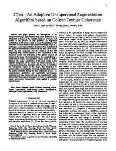
Each individual matching cost score is normalized by its corresponding constant γINV , γICT , γTADC , and γTADG , to ensure equal contribution to the final cost score, or tuned differently to adjust their impact on the matching cost accordingly. Tests of multi-cost function performed on the Middlebury stereo datasets for stereo matching are presented in Figures 5 and 6. The test results show that the matching precision is increased by combining the individual similarity functions. In Figure 5, disparity maps are estimated with different combinations of similarity functions after the aggregation step. From top to bottom: the reference images; the ground truth; the disparity maps estimated by ICT; ICT+TADc; ICT+TADc+TADg; ICT+TADc+TADg+INV; the corresponding bad 2.0 error maps for ICT; ICT+TADc; ICT+TADc+TADg; and ICT+TADc+TADg+INV. The same region of the error maps is marked by red rectangles. The marked regions show that the error is reduced through combining the individual similarity functions. The disparity plane fitting and optimization steps described in Sections 3.3 and 3.4 have not been used here, in order to illustrate individual results and the improvement achieved by fusing the four similarity functions. Figure 6 shows the visualized quantitative performance of similarity functions (in % of erroneous disparities at 2 error threshold) by comparing different combinations of similarity functions against the ground truth. From left to right, the charts correspond to the error matching rate of (a) non-occluded pixels and (b) all image pixels. On the horizontal axis, A: ICT; B: ICT+TADc; C: ICT+TADc+TADg; and D: ICT+TADc+TADg+INV. Following that, the matching cost CRAW ( x, y, d) is stored in a 3D matrix known as the disparity space image (DSI).

Symmetry 2016, 8, 159 Symmetry 2016, 8, 159 

8 of 22 8 of 22 

  Figure 5. Comparison of different ways of similarity functions combination for Middlebury stereo  Figure 5. Comparison of different ways of similarity functions combination for Middlebury stereo datasets. (a) Jade plant; (b) motorcycle; (c) playroom; (d) play table; and (e) shelves. Disparity maps  datasets. (a) Jade plant; (b) motorcycle; (c) playroom; (d) play table; and (e) shelves. Disparity maps are estimated by different combinations of similarity functions after the aggregation step. From top  are estimated by different combinations of similarity functions after the aggregation step. From top to bottom: the reference images; the ground truth; the disparity maps estimated by ICT; ICT+TADc;  to bottom: the reference images; the ground truth; the disparity maps estimated by ICT; ICT+TADc; ICT+TADc+TADg; ICT+TADc+TADg+INV; the corresponding bad 2.0 error maps for ICT; ICT+TADc;  ICT+TADc+TADg; ICT+TADc+TADg+INV; the corresponding bad 2.0 error maps for ICT; ICT+TADc; ICT+TADc+TADg; and ICT+TADc+TADg+INV. The same region of the error maps is marked by red  ICT+TADc+TADg; and ICT+TADc+TADg+INV. The same region of the error maps is marked by rectangles.  red rectangles.

Symmetry 2016, 8, 159 Symmetry 2016, 8, 159 

9 of 22 9 of 22 

  Figure 6.6. The The  visualized  quantitative  performance  of  similarity  functions  (in  %  of  disparities erroneous  Figure visualized quantitative performance of similarity functions (in % of erroneous disparities at 2 error threshold) by comparing different combinations of similarity functions against  at 2 error threshold) by comparing different combinations of similarity functions against the ground the  ground  truth.  From  the left charts to  right,  the  charts  to  the  error  matching  rate  of  (a) pixels non‐ truth. From left to right, correspond tocorrespond  the error matching rate of (a) non-occluded occluded  pixels  and  (b)  all  image  pixels.  On  the  horizontal  axis,  A:  ICT;  B:  ICT+TADc;  C:  and (b) all image pixels. On the horizontal axis, A: ICT; B: ICT+TADc; C: ICT+TADc+TADg; and D: ICT+TADc+TADg; and D: ICT+TADc+TADg+INV.  ICT+TADc+TADg+INV.

3.2.2. Cost Aggregation  3.2.2. Cost Aggregation y ,called d)   is raw called  since  accompanied it  is  always  As mentioned mentioned  above,  matching  cost  (Cx,RAW As above, matching cost C y, (dx),is DSI raw  since DSI  it is always RAW accompanied  with  aliasing  and  noise.  Cost  aggregation  can  decrease  and  noise  by  with aliasing and noise. Cost aggregation can decrease the aliasing and noisethe  by aliasing  averaging or summing averaging or summing up the DSI over a support window. This implicitly assumes that the support  up the DSI over a support window. This implicitly assumes that the support window is a front window is a front parallel surface and all pixels in the window have similar disparities. In order to  parallel surface and all pixels in the window have similar disparities. In order to obtain accurate obtain  accurate  disparity  results  at  near  depth  discontinuities,  an window appropriate  support  window  disparity results at near depth discontinuities, an appropriate support should be constructed. should  be  constructed.  adaptive  cross‐based  that  relies cross on  a  skeleton linearly  expanded  cross  An adaptive cross-basedAn  window that relies on a window  linearly expanded support region skeleton  support  region  for  cost  aggregation  adopted  [7,10,18,28].  The  shape  of  the isadaptive  for cost aggregation is adopted [7,10,18,28]. Theis shape of the adaptive support window visually support window is visually presented in the fifth line of Figure 4. The cross‐based region consists of  presented in the fifth line of Figure 4. The cross-based region consists of multiple horizontal line multiple horizontal line segments spanning several neighboring rows. This aggregation strategy has  segments spanning several neighboring rows. This aggregation strategy has two main advantages: two main advantages: firstly, the support window can vary adaptively, with arbitrary size and shape  firstly, the support window can vary adaptively, with arbitrary size and shape according to the scene according to the scene color similarity; secondly, the aggregation over irregularly shaped support  color similarity; secondly, the aggregation over irregularly shaped support windows can be performed quickly by utilizing the integral image technique. windows can be performed quickly by utilizing the integral image technique.  The construction of cross-based support regions is achieved The construction of cross‐based support regions is achieved by expanding around each pixel a  n o by expanding around each pixel a    + − + − cross‐shaped  skeleton  to  create  four  segments  of  { h , h , v , v } cross-shaped skeleton to create four segments h p p, h pp pp , vpp   defining  defining the  the corresponding  corresponding sets  sets of pixels H(p) and V(p) in the horizontal and vertical directions, as seen in Figure 7a [7]. pixels H(p) and V(p) in the horizontal and vertical directions, as seen in Figure 7a [7].   n o  y )|∈x  , x  h  ], y  y p } y  H ( p) H=( p) (x,{(yx), x p , xp + ph + ], y = [ x[px p− hh− p p p p  n o , y )| x  x p , y  [ y p  v p − , y  v  ]}  V ( p) V=( p) (x,{(yx), x = x p , y ∈ [y p − v p ,py p +p v+ p]

(11) (11)

In our approach, the linear threshold proposed in [7] is used to expand the skeleton around each  In our approach, the linear threshold proposed in [7] is used to expand the skeleton around each pixel:  T(Lq)  =  −(Tmax/Lmax)  ×  Lq  +  Tmax.  This  linear  threshold  T(Lq)  in  color  similarity  involves  the  pixel: T(Lq ) = −(Tmax /Lmax ) × Lq + Tmax . This linear threshold T(Lq ) in color similarity involves the maximum semi‐dimension Lmax of the support window size, the maximum color dissimilarity Tmax  maximum semi-dimension Lmax of the support window size, the maximum color dissimilarity Tmax between pixels p and q, and the spatial closeness Lq. According to [7], the values of Tmax and Lmax are  between pixels p and q, and the spatial closeness Lq . According to [7], the values of Tmax and Lmax are 20 and 35, respectively. The final support window U(p) for p is formulated as a union of horizontal  20 and 35, respectively. The final support window U(p) for p is formulated as a union of horizontal segment H(q), in which q traverses the vertical segment V(p). A symmetric support window is also  segment H(q), in which q traverses the vertical segment V(p). A symmetric support window is also adopted to avoid distortion by the outliers in the reference image [7]. This is shown in Figure 7b.  adopted to avoid distortion by the outliers in the reference image [7]. This is shown in Figure 7b. U ( p)   H ( q ) (12) qV ( p ) U ( p ) = ∪ H ( q ), (12) q ∈V ( p ) The final aggregation cost for each pixel is calculated by aggregating the matching cost over the  support window. This process can be quickly realized by integrating image technology, as shown in  Figure 7c. 

Symmetry 2016, 8, 159

10 of 22

The final aggregation cost for each pixel is calculated by aggregating the matching cost over the Symmetry 2016, 8, 159  10 of 22  support window. This process can be quickly realized by integrating image technology, as shown in Figure 7c. 11 Caggregation ( x p(,xypp, ,ydp ), d= CRAW (13) ) ( xi , y( ix,id, )yi , d), Caggregation C RAW ∑ (13) |U ) ((xxi ,iy,yi )i)∈ U((pp)| U(U p ) ( p)

  Figure 7. The illustration of the adaptive cross‐based aggregation algorithm. (a) The upright cross skeleton.  Figure 7. The illustration of the adaptive cross-based aggregationnalgorithm. (a) The upright cross skeleton. o [xp  hp , xp− hp ], y +yp }   and  a  )|yx) The  upright  H ( pH) ( p= ) {( The upright cross  cross consists  consistsof  ofa ahorizontal  horizontalsegment segment = x, y ( x, x ∈ [ x p − h p , x p + h p ], y = y p n o x y)x xp , = y x[py, py ∈v[py,py−  v− ]} v+ support  region region U(P)  U(P) is  a  vertical  segment and a vertical segment V ( p{()x=, y)|( x, ; (b) the support V ( p )   =  p v pp, y p ; +(b)  p ]the  is a combination of each horizontal segment where q traverses the vertical segment V(p) of p; combination  of  each  horizontal  segment  H(q), H(q), where  q  traverses  the  vertical  segment  V(p)  of  p;  (c)  a  (c) a schematic of a 1D integral image technique. schematic of a 1D integral image technique. 

Subsequently, the initial disparity d x,y at coordinates (x,y) is estimated by using the WTA strategy  Subsequently, the initial disparity dx,y at coordinates (x,y) is estimated by using the WTA strategy where the lowest matching cost is selected:  where the lowest matching cost is selected:

 arg min C C aggregation ( x(,x, y ,y, d )d.), ,y d x,ydx= argmin aggregation D d D min

max

(14) (14)

Dmin ≤d≤ Dmax

3.3. Disparity Plane Fitting 3.3. Disparity Plane Fitting  Although the RANSAC algorithm has been widely used for rejecting outliers fitting data, it is Although the RANSAC algorithm has been widely used for rejecting outliers fitting data, it is  usually not suitable for the segmentation-based framework of stereo matching [13]. That is because usually not suitable for the segmentation‐based framework of stereo matching [13]. That is because  the outliers are caused by many different factors, like textureless areas, occlusion, etc. If the filtering the outliers are caused by many different factors, like textureless areas, occlusion, etc. If the filtering  criteria are different, that produces different outliers. In this section, an iterative outlier suppression criteria are different, that produces different outliers. In this section, an iterative outlier suppression  and disparity plane parameters fitting algorithm is designed for plane fitting. The disparity of each and disparity plane parameters fitting algorithm is designed for plane fitting. The disparity of each  segment region can be modeled as: segment region can be modeled as:  d( x, y) = ax + by + c, (15) d( x, y)  ax  by  c , (15) where d is the corresponding disparity of pixel (x,y), and a, b, c are the plane parameters of the arbitrary where  d  region. is  the  corresponding  disparity  of  pixel  (x,y),  and  a,  b,  c system are  the for plane  parameters  of  the  segment In order to solve the plane parameters, a linear the arbitrary segment arbitrary segment region. In order to solve the plane parameters, a linear system for the arbitrary  region can be formulated as follows: segment region can be formulated as follows:  A[ a, b, c] T = B, (16) ]T  B ,  i0 th element of the vector B is d( x(16) where the i0 th row of the matrix A is [ xi , A yi[,a1, ]b,, cand the i , y i ). Then the linear system can be transformed into the form of A T A[ a, b, c] T = A T B; the detailed function where the  i ʹ th   row of the matrix A is  [ xi , yi ,1] , and the  i ʹ th   element of the vector B is  d( xi , yi ) .  is expressed as follows: T T T Then the linear system can be transformed into the form of     A A[a, b , c ]  A B; the detailed function  m 2 a ∑im=1 xi yi ∑im=1 xi ∑ m xi di is expressed as follows: ∑i=1 xi    im=1   m m m 2 (17)  ∑i=1 xi ym i 2 ∑i=1 ymi ∑i=1 ymi   b  =  m∑i=1 yi di ,     x x y x x d m i 1 i m i  1 i i  i  1 i mi   a   i 1 i 1 ∑i=1 xi ∑ i =1 y i ∑i=1di  c   m m 2   i  1 xi y i  i  1 y i (17)  im1 yi  b     im1 yi di  ,  m  c   m  m 1      i 1 di   i 1 yi   i 1 xi

where m is the number of pixels inside the corresponding segment region. After that, the Singular  Value Decomposition (SVD) approach is employed to solve the least square equation to obtain the  disparity plane parameters: 

Symmetry 2016, 8, 159

11 of 22

where m is the number of pixels inside the corresponding segment region. After that, the Singular Value Decomposition (SVD) approach is employed to solve the least square equation to obtain the disparity plane parameters: + [ a, b, c] T = ( A T A) A T B, (18) +

where ( A T A) is the pseudo-inverse of A T A and can be solved through SVD. However, as is well known, the least square solution is extremely sensitive to outliers. The outliers in this stage are usually generated at the last stage due to the matching error inevitable in initial disparity map estimation. In order to filter out these outliers and obtain accurate plane parameters, four filters are combined. The first filter is mutual consistency check (often called left-right check). The principle of mutual consistency check is that the same point of the stereo image pair should have the same disparity. Thus, the occluded pixels in the scene can be filtered out. Let Dreference be the disparity map from reference image to target image, and Dtarget be the disparity map from target image to reference image. The mutual consistency check is formulated as: Dre f erence ( x, y) − Dtarget ( x − Dre f erence ( x, y), y) ≤ tconsistency ,

(19)

where tconsistency is a constant threshold (typically 1). If the pixels of the reference image satisfy Equation (19), these pixels are marked as non-occluded pixels; otherwise these pixels are marked as occluded pixels, which should be filtered out as outliers. Afterwards, correlation confidence filter is established to judge whether the non-occluded pixels are reliable. Generally, some of the disparity in the textureless areas may be incorrect but will be consistent for both views. Thus, the correlation confidence filter is adopted to overcome this difficulty f irst and obtain reliable pixels. Let Caggregation ( x, y) be the best cost score of a pixel in the non-occluded second pixels set, and Caggregation ( x, y) be the second best cost score of this pixel. The correlation confidence filter is formulated as: C f irst second ( x, y) aggregation ( x, y) − Caggregation ≥ tcon f idence , (20) second Caggregation ( x, y)

where tconfidence is a threshold to adjust the confidence level. If the cost score of the pixels in the reference image satisfies Equation (20), these pixels are considered reliable. If the ratio between the number of the reliable pixels and the total number of the pixels in arbitrary segment region is equal to or greater than 0.5, this segment region is considered a reliable segment region. Otherwise segment regions are marked as unreliable regions, which lack sufficient data to provide reliable plane estimations. The disparity plane of the unreliable region is stuffed through its nearest reliable segment region. Followed by the above filters, the initial disparity plane parameters of each reliable segment region can be estimated through the reliable pixels. The disparity distance filter is adopted to measure the Euclidean distance between initial disparity and the estimated disparity plane:

|d( x, y) − ( ax + by + c)| ≤ toutlier ,

(21)

where toutlier is a constant threshold (typically 1). If the pixel does not satisfy Equation (21), it would be an outlier. Then we can exclude the outliers, update the reliable pixels of the segment region, and re-estimate the disparity plane parameters of the segment region. After the abovementioned three filters, the convergence filter is utilized to judge whether disparity plane is convergent. The new disparity plane parameters will be estimated until: 0 a − a + b0 − b + c0 − c ≤ tconvergence ,

(22)

Symmetry 2016, 8, 159

12 of 22

where (a’,b’,c’) are the parameters of the new disparity plane, (a,b,c) are the parameters of the plane obtained in the previous iteration, and tconvergence is the convergence threshold of the iterative and is usually set as (typically 10−6 ). The flow chart of the iterative outlier suppression and disparity plane parameters fitting algorithm is shown in Figure 8. The detailed implementation of the algorithm is presented as follows, from Step (1) to Step (6): Symmetry 2016, 8, 159  12 of 22 

  Figure 8. The flow chart of the iterative outlier suppression and disparity plane parameters fitting  Figure 8. The flow chart of the iterative outlier suppression and disparity plane parameters algorithm.  fitting algorithm.

Step (1): Input segmented reference image, disparity map of stereo image pair, and the DSI of  Step (1): Input segmented reference image, disparity map of stereo image pair, and the DSI of the the reference image.  reference Step image. (2):  Mutual  consistency  filter  is  utilized  to  check  the  initial  disparity  of  each  pixel  as  in  Step (2): Mutual consistency filter is utilized to check the initial disparity of each pixel as in Equation (19); the pixels are detected as non‐occluded or occluded pixels.  Equation (19); are detected as non-occluded or occluded pixels. Step  (3):  the The pixels reliable  pixels  and  reliable  segment  region  are  determined  by  a  correlation  confidence filter, as in Equation (20).  Step  (4):  The  initial  disparity  plane  parameters  of  each  reliable  segment  region  are  estimated  through the reliable pixels, and the disparity distance filter described in Equation (21) is utilized to  update the reliable pixels.  Step (5): Iterate Step (4) until the convergence filter is satisfied. 

Symmetry 2016, 8, 159

13 of 22

Step (3): The reliable pixels and reliable segment region are determined by a correlation confidence filter, as in Equation (20). Step (4): The initial disparity plane parameters of each reliable segment region are estimated through the reliable pixels, and the disparity distance filter described in Equation (21) is utilized to update the reliable pixels. Step (5): Iterate Step (4) until the convergence filter is satisfied. Step (6): The algorithm will be terminated when the disparity plane parameters of all segment regions have been estimated. Otherwise, return to Step (3) to process the remainder of the reliable segment regions. 3.4. Disparity Plane Optimization by Belief Propagation The last step of the segmentation-based stereo matching algorithm is usually global optimization. The stereo matching is formulated as an energy minimization problem in the segment domain. We label each segment region with its corresponding disparity plane by using the BP algorithm [25]. Assume that each segment region s ∈ R, R is the reference image, its corresponding plane f (s) ∈ D, and D is the disparity plane set. The energy function for labeling f can be formulated as: ETOTAL ( f ) = EDATA ( f ) + ESMOOTH ( f ) + EOCCLUSION ( f ),

(23)

where ETOTAL ( f ) is the whole energy function, EDATA ( f ) is the data term, ESMOOTH ( f ) is the smoothness penalty term, and EOCCLUSION ( f ) is the occlusion penalty term. The data term EDATA ( f ) is formulated for each segment region and its corresponding disparity plane assignment. It is calculated by summing up the matching cost of each segment region: EDATA ( f ) =

∑ CSEG (s, f (s)),

(24)

s∈ R

where CSEG (s, f (s)) is the summation of matching cost, which is defined in Section 3.2 for all the reliable pixels inside the segment: CSEG (s, f (s)) =

∑

C ( x, y, d),

(25)

( x,y)∈s

The smoothness penalty term ESMOOTH ( f ) is used to punish the adjacent segment regions with different disparity plane: ESMOOTH ( f ) =

∑

λdisc (si , s j ),

(26)

(∀(si ,s j )∈S N | f (si )6= f (s j ))

where SN is a set of all adjacent segment regions, Si , Sj are neighboring segment regions, and λdisc ( x, y) is a discontinuity penalty function. The occlusion penalty term EOCCLUSION ( f ) is used to punish the occlusion pixels of each segment region: EOCCLUSION ( f ) = ∑ ωocc Nocc , (27) s∈ R

where ωocc is a coefficient for occlusion penalty and Nocc is the number of occluded pixels of the segment region. The energy function ETOTAL ( f ) is minimized by a BP algorithm, and the final disparity map can be obtained. 4. Experimental Results The proposed stereo matching algorithm has been implemented by VS2010, and the performance of the algorithm is evaluated using the 2014 Middlebury stereo datasets [29], 2006 [30], 2005 [4], the synthesized stereo image pairs [31], and the real-world stereo image pairs. The set of parameter

Symmetry 2016, 8, 159

14 of 22

values used in this paper are shown in Table 1, and the results are shown in Figure 9. The average error rate of the stereo pairs for each evaluation area (all, non-occlusion) are displayed. The percentage of erroneous pixels in the complete image (all) and no-nocclusion areas (nonocc) for the 2 pixels threshold Symmetry 2016, 8, 159  14 of 22  is counted. Figure 9 illustrates the stability of the algorithm to parameter tuning. The test results show that the algorithm isTable 1.  stable Parameters values used for all stereo image pairs.  within a wide range of values for each parameter. We choose the parameters corresponding to the minimum error rate for all the tested stereo image datasets. Parameter Name  Purpose Algorithm Steps Parameter Value  Spatial bandwidth hs  10  Image segmentation  Table 1. Parameters values used for all stereoStep (1)  image pairs. Spectral bandwidth hr  7 

Gamma  γ INV   Parameter Name Gamma  γ   Spatial bandwidth hs ICT Spectral bandwidth hrTADC   Gamma  γ

Purpose

Algorithm Steps

Matching cost computation  Image segmentation

Gamma γINV γ   Gamma  TADG Gamma γICT Matching cost computation Threshold  Gamma γTADC t consistency   Gamma γTADG Threshold  tconfidence   Outliers filter and disparity  Threshold tconsistency plane parameters fitting  Threshold  Threshold tcon f idence toutlier   Outliers filter and disparity Threshold toutlier t   plane parameters fitting Threshold  convergence Threshold tconvergence Smoothness penalty  λ disc   Smoothness and occlusion  Smoothness and Smoothness penalty λdisc penalty  occlusion penalty Occlusion penalty ω ωocc   Occlusion penalty  occ

StepStep (2)  (1)

Step (2)

Step (3)  Step (3)

StepStep (4)  (4)

40  Parameter Value 20  10 40  7 20  40 20 1  40 20 0.04  1 1  0.04 10−6  1−6 10 5  5 5  5

  Figure 9. Diagrams presenting the response of the algorithm to the tuning parameters with the rest of 

Figure 9. Diagrams presenting the response of the algorithm to the tuning parameters with the the parameter set remaining constant. The average error rate of the stereo pairs for each evaluation area  rest of the parameter set remaining constant. The average error rate of the stereo pairs for each (all,  nonocc)  is  displayed.  (a)  Spatial  bandwidth  and  (b)  spectral  bandwidth  used  for  image  evaluation area (all, nonocc) is displayed. SpatialINV(Illumination  bandwidth andNormal  (b) spectral bandwidth segmentation  in  Step  1  of  the  algorithm;  (c(a) )  Gamma  Vector);  (d)  Gamma used for image segmentation in Step 1 ofe) Gamma TADC(Truncated Absolute Difference on Color); and ( the algorithm; (c) Gamma INV(Illumination Normal Vector); f)  ICT(Improved Census Transform); ( (d) Gamma ICT(Improved Census Transform); (e) Gamma TADC(Truncated Absolute Difference Gamma TADG(Truncated Absolute Difference on Gradient) used for matching cost computation in Step  on Color); and (f) Gamma TADG(Truncated Absolute Difference on Gradient) used for matching g) Threshold consistency; ( h) threshold confidence; ( i) threshold outlier; and ( j)  (2) of the algorithm. ( threshold convergence used for outliers filter and disparity plane parameters fitting in Step (3) of the  cost computation in Step (2) of the algorithm. (g) Threshold consistency; (h) threshold confidence; algorithm; ( k) smoothness penalty and ( (i) threshold outlier; and (j) thresholdl) occlusion penalty used for smoothness and occlusion penalty  convergence used for outliers filter and disparity plane in Step (4) of the algorithm.  parameters fitting in Step (3) of the algorithm; (k) smoothness penalty and (l) occlusion penalty used for smoothness and occlusion penalty in Step (4) of the algorithm.

Symmetry 2016, 8, 159

15 of 22

Table 2. Quantitative evaluation based on the training set of the 2014 Middlebury stereo datasets at 2 Error Threshold. The best results for each test column are highlighted in bold. Res and Avg represent resolution scale and average error respectively. Adiron, ArtL, Jadepl, Motor, MotorE, Piano, PianoL, Pipes, Playrm, Playt, PlaytP, Recyc, Shelvs, Teddy, and Vintge are the names of experimental data in the training set. Name

Res

Avg

Adiron

ArtL

Jadepl

Motor

MotorE

Piano

PianoL

Pipes

Playrm

Playt

PlaytP

Recyc

Shelvs

Teddy

Vintge

APAP-Stereo [32] PMSC [33] MeshStereoExt [34] MCCNN_Layout NTDE [35] MC-CNN-acrt [36] LPU MC-CNN+RBS [37] SGM [26] TSGO [38] Our method

H H H H H H H H F F Q

7.78 8.35 9.51 9.54 10.1 10.3 10.4 10.9 22.1 31.3 33.9

3.04 1.46 3.53 3.49 4.54 3.33 3.17 3.85 28.4 27.3 36.5

7.22 4.44 6.76 7.97 7.00 8.04 6.83 10 6.52 12.3 20.6

13.5 11.2 18.1 14.0 15.7 16.1 11.5 18.6 20.1 53.1 35.7

4.39 3.68 5.30 3.91 3.97 3.66 5.8 4.17 13.9 23.5 27.6

4.68 4.07 5.88 4.23 4.37 3.76 6.35 4.31 11.7 25.7 30.5

10.7 11.9 8.80 12.6 13.3 12.5 13.5 12.6 19.7 33.4 38.8

16.1 18.2 13.8 15.6 19.3 18.5 26 17.6 33.2 54.5 59

5.35 5.25 8.10 4.56 5.12 4.22 7.4 7.33 15.5 22.5 26.6

10.1 12.6 11.1 12.3 14.4 14.6 15.3 14.8 30 49.6 46.8

8.60 8.03 8.87 14.9 12.1 15.1 9.63 15.6 58.3 45 56.9

8.11 6.89 8.33 12.9 11.7 13.3 6.48 13.3 18.5 27 31.8

7.70 7.58 10.5 7.79 8.35 6.92 10.7 7.32 23.8 24.2 29.6

12.2 31.6 31.2 24.9 33.5 30.5 35.9 30.1 49.5 52.2 53.3

5.16 3.77 4.96 5.20 3.75 4.65 4.19 5.02 7.38 13.3 12.2

7.97 17.9 12.2 17.6 17.8 24.8 21.6 22.2 49.9 57.5 52.8

Table 3. Quantitative evaluation based on the test set of the 2014 Middlebury stereo datasets at 2 Error Threshold. The best results for each test column are highlighted in bold. Austr, AustrP, Bicyc2, Class, ClassE, Compu, Crusa, CrusaP, Djemb, DjembL, Hoops, Livgrm, Nkuba, Plants and Stairs are the names of experimental data in the test set. Name

Res

Avg

Austr

AustrP

Bicyc2

Class

ClassE

Compu

Crusa

CrusaP

Djemb

DjembL

Hoops

Livgrm

Nkuba

Plants

Stairs

PMSC [33] MeshStereoExt [34] APAP-Stereo [32] NTDE [35] MC-CNN-acrt [36] MC-CNN+RBS [37] MCCNN_Layout LPU SGM [26] Our method TSGO [38]

H H H H H H H H F Q F

6.87 7.29 7.46 7.62 8.29 8.62 9.16 10.5 25.3 38.7 39.1

3.46 4.41 5.43 5.72 5.59 6.05 5.53 11.4 45.1 40.4 34.1

2.68 3.98 4.91 4.36 4.55 5.16 5.63 3.18 4.33 20.3 16.9

6.19 5.4 5.11 5.92 5.96 6.24 5.06 8.1 6.87 27.3 20

2.54 3.17 5.17 2.83 2.83 3.27 3.59 6.08 32.2 35.1 43.3

6.92 10 21.6 10.4 11.4 11.1 12.6 20.9 50 55.9 55.4

6.54 8.89 9.5 8.02 8.44 8.91 9.97 9.84 13 22.3 14.3

3.96 4.62 4.31 5.3 8.32 8.87 7.53 6.94 48.1 56.1 54.1

4.04 4.77 4.23 5.54 8.89 9.83 8.86 4 18.3 50.9 49.2

2.37 3.49 3.24 2.4 2.71 3.21 5.79 4.04 7.66 24.2 33.9

13.1 12.7 14.3 13.5 16.3 15.1 23 33.9 29.6 58 66.2

12.3 12.4 9.78 14.1 14.1 15.9 13.6 16.9 36.1 56.3 45.9

12.2 10.4 7.32 12.6 13.2 12.8 15 15.2 31.2 36.5 39.8

16.2 14.5 13.4 13.9 13 13.5 14.7 17.8 24.2 32.1 42.6

5.88 7.8 6.3 6.39 6.4 7.04 5.85 9.12 24.5 38.7 47.2

10.8 8.85 8.46 12.2 11.1 9.99 10.4 11.6 50.2 69.7 52.6

Symmetry 2016, 8, 159 Symmetry 2016, 8, 159 

16 of 22 16 of 22 

Tables 2 and 3 show the performance evaluation on the training set and test set of the Tables 2,3 show the performance evaluation on the training set and test set of the Middlebury  Middlebury stereo datasets from 2014. Error rates in the table are calculated by setting the threshold stereo datasets from 2014. Error rates in the table are calculated by setting the threshold value to a  value to a two-pixel disparity. The best results for each test column are highlighted in bold. In two‐pixel disparity. The best results for each test column are highlighted in bold. In Table 2, APAP‐ Table 2, APAP-Stereo [32], PMSC [33], MeshStereoExt [34], NTDE [35], MC-CNN-acrt [36], Stereo [32], PMSC [33], MeshStereoExt [34], NTDE [35], MC‐CNN‐acrt [36], and MC‐CNN+RBS [37]  and MC-CNN+RBS [37] are the state-of-the-art stereo matching methods of Middlebury Stereo are the state‐of‐the‐art stereo matching methods of Middlebury Stereo Evaluation Version 3, and the  Evaluation Version 3, and the MCCNN_Layout and LPU methods are anonymously published. MCCNN_Layout and LPU methods are anonymously published. SGM is a classical algorithm based  SGM is a classical algorithm based on semi-global matching and mutual information [26]. TSGO is on semi‐global matching and mutual information [26]. TSGO is an accurate global stereo matching  an accurate global stereo matching algorithm based on energy minimization [38]. The results of the algorithm  based  on  energy  minimization  [38].  The  results  of  the  2014  Middlebury  stereo  datasets  2014 Middlebury stereo datasets show that our method is comparable to these excellent algorithms. show  that  our  method  is  comparable  to  these  excellent  algorithms.  Some  disparity  maps  of  these  Some disparity maps of these stereo pairs are presented in Figure 10. The reference images and ground stereo pairs are presented in Figure 10. The reference images and ground truth maps are shown in  truth maps are shown in Figure 10a,b, respectively; the final disparity maps are given in Figure 10c; Figure 10a,b, respectively; the final disparity maps are given in Figure 10c; and the bad matching  and the bad matching pixels are marked in Figure 10d, where a disparity absolute difference greater pixels are marked in Figure 10d, where a disparity absolute difference greater than 2 is counted as  than 2 is counted as error. Figure 10d indicates that our proposed approach has excellent performance, error.  Figure  10d  indicates  that  our  proposed  approach  has  excellent  performance,  especially  in  especially in textureless regions, disparity discontinuous boundaries, and occluded regions. textureless regions, disparity discontinuous boundaries, and occluded regions. 

  Figure 10. Results of Middlebury stereo datasets “Jade plant”, “Motorcycle”, “Playroom”, “Play table”  Figure 10. Results of Middlebury stereo datasets “Jade plant”, “Motorcycle”, “Playroom”, “Play table” and “Shelves” (from top to bottom). (a) Reference images; (b) ground truth images; (c) results of the  and “Shelves” (from top to bottom). (a) Reference images; (b) ground truth images; (c) results of the proposed method; and (d) error maps (bad estimates with absolute disparity error >2.0 are marked in  proposed method; and (d) error maps (bad estimates with absolute disparity error >2.0 are marked black).  in black).

Symmetry 2016, 8, 159  Symmetry 2016, 8, 159

17 of 22  17 of 22

In  order  to  verify  the  effect  and  importance  of  the  four  similarity  functions  during  the  minimization stage, different combinations of similarity functions and different fitting algorithms are  In order to verify the effect and importance of the four similarity functions during the utilized to evaluate the 2014 Middlebury stereo datasets. The statistical results are shown in Figure  minimization stage, different combinations of similarity functions and different fitting algorithms 11.  Firstly,  to the  initial  the disparity  is  estimated  by  datasets. ICT,  ICT+TADc,  ICT+TADc+TADg,  and  are utilized evaluate 2014 Middlebury stereo The statistical results are shown ICT+TADc+TADg+INV,  respectively.  Secondly,  the  disparity  plane  fitting  for  ICT+TADc+TADg, initial  disparity  is  in Figure 11. Firstly, the initial disparity is estimated by ICT, ICT+TADc, performed by RANSAC and our fitting algorithm, respectively. Finally, the corresponding disparity  and ICT+TADc+TADg+INV, respectively. Secondly, the disparity plane fitting for initial disparity is plane  is  optimized  by  BP.  importance  of  the  four  similarity  functions  during  the  performed by RANSAC andThe  oureffect  fittingand  algorithm, respectively. Finally, the corresponding disparity disparity  plane  fitting  and  minimization  stage  can  be similarity observed functions through  during the  histogram.  The  plane is optimized by BP.stage  The effect and importance of the four the disparity results illustrate that the most accurate initial disparity can be estimated by ICT+TADc+TADg+INV,  plane fitting stage and minimization stage can be observed through the histogram. The results illustrate and the most accurate final disparity map can be obtained by optimizing the most accurate initial  that the most accurate initial disparity can be estimated by ICT+TADc+TADg+INV, and the most disparity.  accurate final disparity map can be obtained by optimizing the most accurate initial disparity.

  Figure 11. Figure 11. The statistical results of different combinations of similarity functions and different fitting  The statistical results of different combinations of similarity functions and different fitting algorithms. ( a) The average error rates of the non‐occlusion areas (nonocc) and ( b) of the complete  algorithms. (a) The average error rates of the non-occlusion areas (nonocc) and (b) of the complete image (all). A: initial disparity; B: disparity plane fitting by RANSAC; C: disparity plane optimization  image (all). A: initial disparity; B: disparity plane fitting by RANSAC; C: disparity plane optimization of B; D: disparity plane fitting by our iterative outlier suppression and disparity plane parameters  of B; D: disparity plane fitting by our iterative outlier suppression and disparity plane parameters fitting algorithm; E: disparity plane optimization of D.  fitting algorithm; E: disparity plane optimization of D.

The degree to which each step of the algorithm contributes to the reduction of the disparity error  The degree to which each step of the algorithm contributes to the reduction of the disparity error with respect to ground truth is shown in Figure 12. The disparity results are evaluated on the 2014  with respect to ground truth is shown in Figure 12. The disparity results are evaluated on the 2014 Middlebury stereo datasets. The charts in Figure 12 present the improvement obtained at each step  Middlebury stereo datasets. The charts in Figure 12 present the improvement obtained at each step for for the 0.5, 1.0, 2.0, and 4.0 pixel thresholds. The errors refer to non‐occlusion areas (nonocc) and to  the 0.5, 1.0, 2.0, and 4.0 pixel thresholds. The errors refer to non-occlusion areas (nonocc) and to the the whole image (all). The contribution of each step to disparity improvement is seen at the nonocc  whole image (all). The contribution of each step to disparity improvement is seen at the nonocc and all and all curves. One may observe that the error rate is reduced by adding the algorithm steps.  curves. One may observe that the error rate is reduced by adding the algorithm steps. The results of some representative data of the Middlebury stereo data are presented in Figure  The results of some representative data of the Middlebury stereo data are presented in Figure 13. 13. They are: Moebius and Laundry choose from 2005 Middlebury stereo datasets [4]; Bowling 2 and  They are: Moebius and Laundry choose from 2005 Middlebury stereo datasets [4]; Bowling 2 and Plastic choose from 2006 Middlebury stereo datasets [30]. These stereo pairs are captured by high‐ Plastic choose from 2006 Middlebury stereo datasets [30]. These stereo pairs are captured by high-end end cameras in a controlled laboratory environment. The produced disparity maps are accurate, and  cameras in a controlled laboratory environment. The produced disparity maps are accurate, and the the error rates of the four Middlebury stereo data with reference to the whole image are given as  error rates of the four Middlebury stereo data with reference to the whole image are given as follows: follows:  Moebius,  8.28%;  Laundry,  12.65%;  Bowling  2,  8.5%;  and  Plastic,  13.49%.  Data  Moebius  Moebius, 8.28%; Laundry, 12.65%; Bowling 2, 8.5%; and Plastic, 13.49%. Data Moebius presents an presents an indoor scene with many stacking objects. Our method can generate accurate disparity for  indoor scene with many stacking objects. Our method can generate accurate disparity for most parts most parts of the scene, and the disparity of small toys on the floor is correctly recovered. For data  of the scene, and the disparity of small toys on the floor is correctly recovered. For data Laundry, Laundry, a relatively good disparity map is generated for a laundry basket with repeated textures.  a relatively good disparity map is generated for a laundry basket with repeated textures. In Bowling 2, In Bowling 2, objects with curved surfaces are presented, e.g., ball and Bowling. Disparities of these  objects with curved surfaces are presented, e.g., ball and Bowling. Disparities of these objects are both objects are both accurate and smooth. The disparity of the background (map) is also obtained with  accurate and smooth. The disparity of the background (map) is also obtained with few mismatches. few mismatches. In Plastic, the texture information is much weaker; nevertheless, our method can  In Plastic, the texture information is much weaker; nevertheless, our method can still generate an still generate an accurate and smooth disparity map that is close to the ground truth. These examples  accurate and smooth disparity map that is close to the ground truth. These examples demonstrate the demonstrate the ability of our approach to produce promising results.  ability of our approach to produce promising results.

Symmetry 2016, 8, 159

18 of 22

Symmetry 2016, 8, 159  Symmetry 2016, 8, 159 

18 of 22  18 of 22 

   

Figure  12.  Performance  of  each  step  of  the  algorithm  regarding  disparity  map  accuracy.  (a)  The  Figure 12. each step of the regarding disparity map accuracy. (a) The average Figure  12. Performance Performance ofof  each  step  of  algorithm the  algorithm  regarding  disparity  map  accuracy.  (a)  The  average  error  rates  of  the  complete  image  (all)  and  non‐occlusion  areas (nonocc)  for  the threshold; 0.75  pixel  error rates of the complete image (all) and non-occlusion areas (nonocc) for the 0.75 pixel average  error  rates  of  the  complete  image  (all)  and  non‐occlusion  areas (nonocc)  for  the  0.75  pixel  b) the average error rates of the complete image (all) and non‐occlusion areas (nonocc) for  threshold; ( (b) the average error rates of the complete image (all) and non-occlusion areas (nonocc) for the 1.0 pixel b) the average error rates of the complete image (all) and non‐occlusion areas (nonocc) for  threshold; ( the 1.0 pixel threshold; ( c) the average error rates of the complete image (all) and non‐occlusion areas  threshold; (c) the average error rates of the complete image (all) and non-occlusion areas (nonocc) for the 1.0 pixel threshold; ( c) the average error rates of the complete image (all) and non‐occlusion areas  (nonocc) for the 2.0 pixel threshold; and ( ) the average error rates of the complete image (all) and  the 2.0 pixel threshold; and (d) the averaged error rates of the complete image (all) and non-occlusion (nonocc) for the 2.0 pixel threshold; and ( d) the average error rates of the complete image (all) and  non‐occlusion areas (nonocc) for the 4.0 pixel threshold. A: initial disparity estimation, B: disparity  areas (nonocc) for the 4.0 pixel threshold. A: initial disparity estimation, B: disparity plane fitting, and non‐occlusion areas (nonocc) for the 4.0 pixel threshold. A: initial disparity estimation, B: disparity  plane fitting, and C: disparity plane optimization.  C: disparity plane optimization. plane fitting, and C: disparity plane optimization. 

   

Figure  13.  Results  of  representative  data  on  the  Middlebury  website.  From  top  to  bottom:  Moebius,  Figure  13.  Results Results  of of representative representative  data  on  the the Middlebury Middlebury  website. website.  From  top  to to bottom: bottom:  Moebius, Moebius,  Figure 13. data on From ctop Laundry, Bowling 2 and Plastic. ( a) Reference image; ( b) ground truth images; ( ) results of the proposed  Laundry, Bowling 2 and Plastic. ( a ) Reference image; ( b ) ground truth images; ( c ) results of the proposed  Laundry, Bowling 2 and Plastic. (a) Reference image; (b) ground truth images; (c) results of the method; and ( d) error maps (bad estimates with absolute disparity error >1.0 are marked in black).  method; and ( d) error maps (bad estimates with absolute disparity error >1.0 are marked in black).  proposed method; and (d) error maps (bad estimates with absolute disparity error >1.0 are marked in black). Apart from the Middlebury benchmark images, we also tested the proposed method on both 

Apart from the Middlebury benchmark images, we also tested the proposed method on both  synthesized [31] and real‐world stereo pairs. Figure 14 presents the results of the proposed algorithm  synthesized [31] and real‐world stereo pairs. Figure 14 presents the results of the proposed algorithm  Apartsynthesized  from the Middlebury benchmark images,and  we also tested the proposed method on both on  three  stereo  pairs:  Tanks,  Temple,  Street.  High‐quality  disparity  maps  are  on  three  synthesized  stereo  pairs:  Tanks,  Temple,  and  Street.  High‐quality  disparity  maps  are  synthesized [31] and real-world stereo pairs. Figure 14 presents the results of the proposed algorithm generated and compared with the ground truth in the second column. The produced disparity maps  generated and compared with the ground truth in the second column. The produced disparity maps  on three synthesized stereo and Street. High-quality disparity maps are generated are  accurate,  and  the  error pairs: rates Tanks, of  the Temple, three  synthesized  stereo  pairs  with  reference  to  the  whole  are  accurate,  and  the  error  rates  of  the  three  synthesized  stereo  pairs  with  reference  to  the  whole  and compared with groundTanks,  truth in the second column. Theand  produced are that  accurate, image  are  given  as the follows:  4.42%;  Temple,  2.66%;  Street, disparity 7.93%.  It maps is  clear  our  image  are  given  as  follows:  Tanks,  4.42%;  Temple,  2.66%;  and  Street,  7.93%.  It  is  clear  that  our  algorithm performs well for details, e.g., the gun barrels of the tanks, as well as for large textureless  algorithm performs well for details, e.g., the gun barrels of the tanks, as well as for large textureless  background regions and repetitive patterns.  background regions and repetitive patterns. 

Symmetry 2016, 8, 159

19 of 22

and the error rates of the three synthesized stereo pairs with reference to the whole image are given as follows: Tanks, 4.42%; Temple, 2.66%; and Street, 7.93%. It is clear that our algorithm performs well for details, e.g., the gun barrels of the tanks, as well as for large textureless background regions and repetitive patterns. Symmetry 2016, 8, 159  19 of 22 

Symmetry 2016, 8, 159 

19 of 22 

   

Figure  14. Results  of  synthesized  stereo  pairs.  From  top  to  bottom:  Tanks,  Temple,  and  Street.  (a)  Figure 14. 14.  Results  Resultsof  ofsynthesized  synthesizedstereo  stereopairs.  pairs. From to bottom: Tanks, Temple, Street. Figure  From  top top to  bottom:  Tanks,  Temple,  and and Street.  (a)  b ) ground truth images; ( c ) results of the proposed method; and ( d ) error maps  Reference image; ( (a) Reference image; (b) ground truth images;c) results of the proposed method; and ( (c) results of the proposed method; and d (d) error maps b) ground truth images; ( ) error maps  Reference image; ( (bad estimates with absolute disparity error >1.0 are marked in black).  (bad estimates with absolute disparity error >1.0 are marked in black). (bad estimates with absolute disparity error >1.0 are marked in black). 

The  proposed  algorithm  also  performs  well  on  publicly  available,  real‐world  stereo  video  The  proposed algorithm algorithm  also  performs  on  publicly  available,  real‐world  stereo  video  The proposed also performs wellwell  on publicly available, real-world stereo video datasets: datasets: a “Book Arrival” sequence from FhG‐HHI database and an “Ilkay” sequence from Microsoft  datasets: a “Book Arrival” sequence from FhG‐HHI database and an “Ilkay” sequence from Microsoft  a “Book Arrival” sequence from FhG-HHI database and an “Ilkay” sequence from Microsoft i2i i2i  database.  The  snapshots  for  the  two  video  sequences  and  corresponding  disparity  maps  are  i2i  database.  snapshots  for two the video two  sequences video  sequences  and  corresponding  are  database. TheThe  snapshots for the and corresponding disparitydisparity  maps are maps  presented presented in Figure 15. For both examples, our system performs reasonably well. In this experiment,  presented in Figure 15. For both examples, our system performs reasonably well. In this experiment,  in Figure 15. For both examples, our system performs reasonably well. In this experiment, we did we did not give the error maps and the error rate, due to there being no ground truth disparity map  we did not give the error maps and the error rate, due to there being no ground truth disparity map  not give the error maps and the error rate, due to there being no ground truth disparity map for the for  the  real‐world  stereo  video  datasets.  However,  in  terms  of  the  visual  effect,  the  proposed  for  the  real‐world  stereo  video However, datasets. in However,  in  visual terms  effect, of  the the visual  effect,  the  proposed  real-world stereo video datasets. terms of the proposed algorithm can be algorithm can be applied to this dataset very well.  algorithm can be applied to this dataset very well.  applied to this dataset very well.

   

Figure 15. Results of real‐world stereo data. (a) Frames of ”Book Arrival” stereo video sequence; (b)  Figure 15. b)  Figure 15. Results of real‐world stereo data. ( Results of real-world stereo data.a) Frames of ”Book Arrival” stereo video sequence; ( Framesof  of”Ilkay”  ”Book Arrival” stereo video sequence; estimated  disparity  maps  of  ”Book  Arrival”;  ((a) c)  frames  stereo  video  sequence;  and  (d)  estimated  disparity  maps maps of  ”Book  Arrival”;  (c)  frames  of  ”Ilkay”  stereo  video  and  (d)  (b) estimated disparity of ”Book Arrival”; (c) frames of ”Ilkay” stereosequence;  video sequence; estimated disparity maps of ”Ilkay”.  estimated disparity maps of ”Ilkay”.  and (d) estimated disparity maps of ”Ilkay”.

Runtime. The algorithm implementation is written in VS2010 and uses the OpenCV core library  Runtime. The algorithm implementation is written in VS2010 and uses the OpenCV core library  for basic matrix operations. The runtime is measured on a desktop with Core i7‐6700HQ 2.60 GHz  Runtime. The algorithm implementation is written in VS2010 and uses the OpenCV core library for basic matrix operations. The runtime is measured on a desktop with Core i7‐6700HQ 2.60 GHz  CPU and 16 GB RAM, and no parallelism technique is utilized. All operations are carried out with  for basic matrix operations. The runtime is measured on a desktop with Core i7-6700HQ 2.60 GHz CPU and 16 GB RAM, and no parallelism technique is utilized. All operations are carried out with  floating point precision. Our algorithm require 0.59 s/megapixels (s/mp) for image segmentation, 3.4  floating point precision. Our algorithm require 0.59 s/megapixels (s/mp) for image segmentation, 3.4  s/mp for initial disparity estimation, 15.8 s/mp for disparity plane fitting, and 7.6 s/mp for disparity  s/mp for initial disparity estimation, 15.8 s/mp for disparity plane fitting, and 7.6 s/mp for disparity  plane optimization.  plane optimization.  5. Discussion and Conclusions  5. Discussion and Conclusions 

Symmetry 2016, 8, 159

20 of 22

CPU and 16 GB RAM, and no parallelism technique is utilized. All operations are carried out with floating point precision. Our algorithm require 0.59 s/megapixels (s/mp) for image segmentation, 3.4 s/mp for initial disparity estimation, 15.8 s/mp for disparity plane fitting, and 7.6 s/mp for disparity plane optimization. 5. Discussion and Conclusions In summary, we present a highly accurate solution to the stereo correspondence problem. The main contribution of this work is to integrate the appealing properties of the multi-cost approach into the segmentation-based framework. Our algorithm has two advantages. Firstly, an adaptive multi-cost method for disparity evaluation is designed to ensure the accuracy of the initial disparity map. The combined similarity function increases the robustness of the initial raw matching costs calculation and the adaptive support window effectively reduces the matching ambiguity. Secondly, an iterative outlier suppression and disparity plane parameters fitting algorithm is developed to ensure a reliable pixel set for each segment region and obtain accurate disparity plane parameters. The ability to deal with textureless areas and occlusion is enhanced by segment constraint. The experimental results demonstrated that the proposed algorithm can generate state-of-the-art disparity results. The ideas introduced in this paper could be used or extended in future stereo algorithms in order to boost their accuracy. Acknowledgments: This work was supported by the National Natural Science Foundation of China (Grant No. 11547157 and 61100004), the Natural Science Foundation of Heilongjiang Province of China (Grant No. F201320), and Harbin Municipal Science and Technology Bureau (Grant No. 2014RFQXJ073). Sincere thanks are given for the comments and contributions of anonymous reviewers and members of the editorial team. Author Contributions: Ning Ma proposed the idea for the method. Ning Ma and Yubo Men performed the validation experiment. Ning Ma, Chaoguang Men, and Xiang Li wrote the paper. All the authors read and approved the final paper. Conflicts of Interest: The authors declare no conflict of interest.

References 1. 2. 3. 4. 5. 6.

7. 8. 9. 10.

Scharstein, D.; Szeliski, R. A taxonomy and evaluation of dense two-frame stereo correspondence algorithms. Int. J. Comput. Vis. 2002, 47, 7–42. [CrossRef] Pham, C.C.; Jeon, J.W. Domain transformation-based efficient cost aggregation for local stereo matching. IEEE Trans. Circuits Syst. Video Technol. 2013, 23, 1119–1130. [CrossRef] Wang, D.; Lim, K.B. Obtaining depth map from segment-based stereo matching using graph cuts. J. Vis. Commun. Image Represent. 2011, 22, 325–331. [CrossRef] Scharstein, D.; Pal, C. Learning conditional random fields for stereo. In Proceedings of the IEEE Conference on Computer Vision and Pattern Recognition, Minneapolis, MN, USA, 17–22 June 2007; pp. 1–8. Scharstein, D.; Szeliski, R. High-accuracy stereo depth maps using structured light. In Proceedings of the Computer Vision and Pattern Recognition, Madison, WI, USA, 18–20 June 2003. Shan, Y.; Hao, Y.; Wang, W.; Wang, Y.; Chen, X.; Yang, H.; Luk, W. Hardware acceleration for an accurate stereo vision system using mini-census adaptive support region. ACM Trans. Embed. Comput. Syst. 2014, 13, 132. [CrossRef] Stentoumis, C.; Grammatikopoulos, L.; Kalisperakis, I.; Karras, G. On accurate dense stereo-matching using a local adaptive multi-cost approach. ISPRS J. Photogramm. Remote Sens. 2014, 91, 29–49. [CrossRef] Miron, A.; Ainouz, S.; Rogozan, A.; Bensrhair, A. A robust cost function for stereo matching of road scenes. Pattern Recognit. Lett. 2014, 38, 70–77. [CrossRef] Saygili, G.; van der Maaten, L.; Hendriks, E.A. Adaptive stereo similarity fusion using confidence measures. Comput. Vis. Image Underst. 2015, 135, 95–108. [CrossRef] Stentoumis, C.; Grammatikopoulos, L.; Kalisperakis, I.; Karras, G.; Petsa, E. Stereo matching based on census transformation of image gradients. In Proceedings of the SPIE Optical Metrology, International Society for Optics and Photonics, Munich, Germany, 21 June 2015.

Symmetry 2016, 8, 159

11.

12. 13.

14. 15.

16. 17. 18. 19.

20. 21. 22. 23. 24.

25. 26. 27. 28. 29.

30. 31.

32. 33.

21 of 22

Klaus, A.; Sormann, M.; Karner, K. Segment-based stereo matching using belief propagation and a self-adapting dissimilarity measure. In Proceedings of the IEEE 18th International Conference on Pattern Recognition (ICPR’06), Hong Kong, China, 20–24 August 2006; pp. 15–18. Kordelas, G.A.; Alexiadis, D.S.; Daras, P.; Izquierdo, E. Enhanced disparity estimation in stereo images. Image Vis. Comput. 2015, 35, 31–49. [CrossRef] Wang, Z.F.; Zheng, Z.G. A region based stereo matching algorithm using cooperative optimization. In Proceedings of the IEEE Conference on Computer Vision and Pattern Recognition, Anchorage, AK, USA, 23–28 June 2008; pp. 1–8. Xu, S.; Zhang, F.; He, X.; Zhang, X. PM-PM: PatchMatch with Potts model for object segmentation and stereo matching. IEEE Trans. Image Process. 2015, 24, 2182–2196. [PubMed] Taguchi, Y.; Wilburn, B.; Zitnick, C.L. Stereo reconstruction with mixed pixels using adaptive over-segmentation. In Proceedings of the IEEE Conference on Computer Vision and Pattern Recognition, Anchorage, AK, USA, 23–28 June 2008; pp. 1–8. Damjanovi´c, S.; van der Heijden, F.; Spreeuwers, L.J. Local stereo matching using adaptive local segmentation. ISRN Mach. Vis. 2012, 2012, 163285. [CrossRef] Yoon, K.J.; Kweon, I.S. Adaptive support-weight approach for correspondence search. IEEE Trans. Pattern Anal. 2006, 28, 650–656. [CrossRef] [PubMed] Zhang, K.; Lu, J.; Lafruit, G. Cross-based local stereo matching using orthogonal integral images. IEEE Trans. Circuits Syst. Video Technol. 2009, 19, 1073–1079. [CrossRef] Veksler, O. Fast variable window for stereo correspondence using integral images. In Proceedings of the 2003 IEEE Computer Society Conference on Computer Vision and Pattern Recognition, Madison, WI, USA, 18–20 June 2003. Okutomi, M.; Katayama, Y.; Oka, S. A simple stereo algorithm to recover precise object boundaries and smooth surfaces. Int. J. Comput. Vis. 2002, 47, 261–273. [CrossRef] Hosni, A.; Rhemann, C.; Bleyer, M.; Rother, C.; Gelautz, M. Fast cost-volume filtering for visual correspondence and beyond. IEEE Trans. Pattern Anal. 2013, 35, 504–511. [CrossRef] [PubMed] Gao, K.; Chen, H.; Zhao, Y.; Geng, Y.N.; Wang, G. Stereo matching algorithm based on illumination normal similarity and adaptive support weight. Opt. Eng. 2013, 52, 027201. [CrossRef] Wang, L.; Yang, R.; Gong, M.; Liao, M. Real-time stereo using approximated joint bilateral filtering and dynamic programming. J. Real-Time Image Process. 2014, 9, 447–461. [CrossRef] Taniai, T.; Matsushita, Y.; Naemura, T. Graph cut based continuous stereo matching using locally shared labels. In Proceedings of the IEEE Conference on Computer Vision and Pattern Recognition, Columbus, OH, USA, 23–28 June 2014; pp. 1613–1620. Besse, F.; Rother, C.; Fitzgibbon, A.; Kautz, J. Pmbp: Patchmatch belief propagation for correspondence field estimation. Int. J. Comput. Vis. 2014, 110, 2–13. [CrossRef] Hirschmuller, H. Stereo Processing by Semiglobal Matching and Mutual Information. IEEE Trans. Pattern Anal. 2008, 30, 328–341. [CrossRef] [PubMed] Comaniciu, D.; Meer, P. Mean shift: A robust approach toward feature space analysis. IEEE Trans. Pattern Anal. 2002, 24, 603–619. [CrossRef] Yao, L.; Li, D.; Zhang, J.; Wang, L.H.; Zhang, M. Accurate real-time stereo correspondence using intra-and inter-scanline optimization. J. Zhejiang Univ. Sci. C 2012, 13, 472–482. [CrossRef] Scharstein, D.; Hirschmüller, H.; Kitajima, Y.; Krathwohl, G.; Neši´c, N.; Wang, X.; Westling, P. High-resolution stereo datasets with subpixel-accurate ground truth. In Proceedings of the German Conference on Pattern Recognition, Münster, Germany, 2–5 September 2014; pp. 31–42. Hirschmuller, H.; Scharstein, D. Evaluation of cost functions for stereo matching. In Proceedings of the IEEE Conference on Computer Vision and Pattern Recognition, Minneapolis, MN, USA, 17–22 June 2007; pp. 1–8. Richardt, C.; Orr, D.; Davies, I.; Criminisi, A.; Dodgson, N.A. Real-time spatiotemporal stereo matching using the dual-cross-bilateral grid. In Proceedings of the European Conference on Computer Vision, Crete, Greece, 5–11 September 2010; pp. 510–523. Park, M.G.; Yoon, K.J. As-planar-as-possible depth map estimation. IEEE Trans. Pattern Anal. 2016, submitted. Li, L.; Zhang, S.; Yu, X.; Zhang, L. PMSC: PatchMatch-based superpixel cut for accurate stereo matching. IEEE T. Circ. Syst. Vid. 2016. [CrossRef]

Symmetry 2016, 8, 159

34.

35.

36. 37. 38.

22 of 22

Zhang, C.; Li, Z.; Cheng, Y.; Cai, R.; Chao, H.; Rui, Y. Meshstereo: A global stereo model with mesh alignment regularization for view interpolation. In Proceedings of the IEEE International Conference on Computer Vision, Santiago, Chile, 13–16 December 2015; pp. 2057–2065. Kim, K.R.; Kim, C.S. Adaptive smoothness constraints for efficient stereo matching using texture and edge information. In Proceedings of the Image Processing (ICIP), Phoenix, AZ, USA, 25–28 September 2016; pp. 3429–3433. Zbontar, J.; LeCun, Y. Stereo matching by training a convolutional neural network to compare image patches. J. Mach. Learn. Res. 2016, 17, 1–32. Barron, J.T.; Poole, B. The Fast Bilateral Solver. In Proceedings of the European Conference on Computer Vision, Amsterdam, The Netherlands, 11–14 October 2016; pp. 617–632. Mozerov, M.G.; van de Weijer, J. Accurate stereo matching by two-step energy minimization. IEEE Trans. Image Process. 2015, 24, 1153–1163. [CrossRef] [PubMed] © 2016 by the authors; licensee MDPI, Basel, Switzerland. This article is an open access article distributed under the terms and conditions of the Creative Commons Attribution (CC-BY) license (http://creativecommons.org/licenses/by/4.0/).