Splat-based Ray Tracing of Point Clouds Lars Linsen∗ ∗
Karsten M¨uller†
School of Enginieering and Science International University Bremen‡ Bremen, Germany
†
Paul Rosenthal∗
Department of Mathematics and Computer Science Ernst-Moritz-Arndt-Universit¨at Greifswald Greifswald, Germany
ABSTRACT Point-based surface representations have gained increasing interest in the computer graphics community within the last decade. Surface splatting established as one of the main rendering techniques for point clouds. We present a ray-tracing approach for objects whose surfaces are represented by point clouds. Our approach is based on casting rays and intersecting them with splats. Since ray-tracing methods require smoothly changing surface normals for producing the desired photorealistic results, splat generation must include the derivation of such normals. We determine a neighborhood around each point of the point cloud, estimate the surface normal at each of the points, compute splats with varying radii that cover the surface, and use the normals of all points that are covered by each splat to generate a smoothly varying normal field for each splat. This part of the computation is view-independent and, thus, can be precomputed. During the rendering step, ray-splat intersections are performed, where the normal at the intersection point is interpolated using local coordinates of the splat’s normal field. Care has to be taken where splats overlap. We speed up the computations of the ray-splat intersections using an octree data structure. Keywords: Point-based rendering, ray tracing, splatting, photo-realistic rendering.
1 Introduction Ray tracing is a well-known and widely used technique in computer graphics for photo-realistic rendering of three-dimensional scenes with multiple objects and light sources. It allows for precise shadow computations and modeling of light reflection and refraction. The objects are typically described by their boundary surfaces, which can be given in implicit or explicit form. Often implicit representations of the boundary surfaces are unknown. Therefore, explicit representations in form of triangular (or polygonal) meshes are most commonly used to describe the surfaces. Ray tracing of scenes using triangular mesh representations has a long tradition in photo-realistic rendering. The main approach [App68, Whi80] is described in any computer graphics textbook, e. g. [Wat00]. With the upcoming of precise high-resolution 3D laser scanning techniques about a decade ago, point-based explicit surface representations have gained major interest in the computer graphics society. Surfaces of real objects are sampled leading to a large number of typically unstructured points lying on the surface. This set of points is often referred to as a point cloud. A pioneer project describing such efforts was the Michelangelo project [LPC+ 00]. ∗ {l.linsen,
p.rosenthal}@iu-bremen.de
†
[email protected] ‡ Jacobs
University Bremen as of Spring 2007.
Permission to make digital or hard copies of all or part of this work for personal or classroom use is granted without fee provided that copies are not made or distributed for profit or commercial advantage and that copies bear this notice and the full citation on the first page. To copy otherwise, or republish, to post on servers or to redistribute to lists, requires prior specific permission and/or a fee. Copyright UNION Agency - Science Press, Plzen, Czech Republic.
Instead of converting point clouds to polygonal representations, several efforts have been made to directly render surfaces using point clouds for surface representation [Lin01, PZvBG00, RL00]. For an overview over current directions in the field of point-based computer graphics, we refer to the tutorial by Gross et al. [AGP+ 04]. Two main streams of point-based rendering methods have emerged, namely the surface splatting approach [ZPvBG01] and the point set surface approach [ABCO+ 01]. The surface splatting approach is based on computing a surface normal at each sample’s surface point and a radial or elliptical expansion tangential to the surface. The generated discs are the so-called splats. They are supposed to overlap in order to cover the entire surface of the scanned object. The point set surface approach, on the other hand, is based on the moving least-squares surface definition [Lev03]. The surface is locally reconstructed by fitting a polynomial to the sample points within a small neighborhood surrounding a given point. The given point is projected onto an implicitely defined polynomial surface. The point set surface is defined as the set of points that project onto themselves. The splatting approach is much simpler in its mathematical formulation, but the point-set-surface approach generates continuous surface representations, which makes it amenable to photo-realisitic rendering [AA03]. However, when looking into computation complexity, the algorithms of splat-based approaches are, in general, much less computationally intense. We exploited the simplicity of splat-based surface representations to develop an efficient ray-tracing approach for point clouds. Splats in their general form define a piece-wise con-
stant surface. In particular, each splat has exactly one surface normal assigned to it. Assuming that the point cloud was obtained by scanning a smooth surface, the application of our rendering technique should result in the display of a smoothly varying surface. Since ray tracing is based on casting rays, whose directions depend on the surface normals, we need to define smoothly varying normals over the entire surface, i. e. also within each splat. To do so, we consider the estimated normals at each point of the point cloud and compute splat radii depending on local curvature properties. The generated splats should cover several points of the point cloud. The normals at the covered points of each splat are used to determine a smoothly varying normal field defined over a local parameter space of the splat. It can be beneficial to consider further surrounding points and their normals for the normal field computations. Details on the splat and normal field generation are described in Section 3. The actual ray-tracing procedure is executed by sending out rays that intersect the splats, potentially being reflected or refracted. Surface normals are interpolated from the normal fields. Care has to be taklen where splats overlap. The ray-splat intersection and the overall image generation is described in Section 4. Primary and secondary rays are treated equally. We use an octree-based approach to improve the performance of our approach in terms of computation time. Since our splat-based surface generation is viewindependent, the computation of the splats and the normal field can be executed in a preprocessing step. Thus, during an animation, only the ray-splat intersections have to be computed for each frame, which significantly reduces the computation times. We achieved to efficiently produce photo-realistic images including reflective and transmittive surfaces similar to the images generated by mesh-based ray-tracing methods. Our results are shown and discussed in Sections 5 and 6. Moreover, our approach is general enough to allow for the combination with any further improvements known from mesh-based ray tracing.
2 Related Work Schaufler and Jensen [SJ00] were the first to propose a ray-tracing technique for point clouds. Their idea is based on sending out rays with a certain width which can geometrically be described as cylinders. The intersection detection is performed by determining the points of the point cloud that lie within such a cylinder followed by calculating the ray-surface intersection point as distance-weighted average of the locations of these points. The normal information at the intersection point is determined using the same weighted averaging. This approach does not handle varying point density within the point cloud. Moreover, the surface generation is view-dependent, which may lead to artifacts during animations. Wand and Straßer [WS03] introduce a similar concept by replacing the cylinders with cones. By using Gaussian weighting of the points within the cone they obtain anti-aliased images. To speed up their method they used a multi-resolution approach. Starting with a set of
triangles and based on their multi-resolution hierarchy and a Gaussian filter, they precompute a uniformly distributed representative point cloud from the triangles with average surface properties. Thus, the generated point cloud has certain known properties and the surface properties are fixed. Hence, when changing material properties etc., the rather expensive preprocessing steps have to be recomputed. Adamson and Alexa [AA03] proposed a method for ray tracing point set surfaces. For the intersection of the rays with the locally reconstructed surfaces, points on the ray are iteratively projected onto the surface until the procedure converges. Obviously, this is a computationally intense approach. The authors state that the computation times for all their presented examples were in the range of several hours. An interactive ray tracing algorithm of point-based models was introduced by Wald and Seidel [WS05]. They experimented with implicite surface and splatbased approaches. The former turned out to be too computationally expensive for interacive ray tracing. However, the method proposed by Wald and Seidel only used ray tracing for shadow computation, the actual shading is performed using local shading models. Thus, transparency and mirroring reflections are not modeled. Our method instead allows for the generation of such ray tracing-specific properties up to any given ray trace depth. Nevertheless, the ray tracing-step introduced by Wald and Seidel can be adopted to generate such images, as well. We incorporated their approach into our frame work to compare them in terms of quality and speed. It turned out that our ray tracing-step is favorable in both categories, see Section 6.
3 Splat Generation Let P be a point cloud consisting of n points p1 , . . . , pn ∈ ℜ3 . We generate m splats S1 , . . . , Sm that cover the entire surface represented by point cloud P. For each of these splats we are computing its radius ri ∈ ℜ, i = 1, . . . , m, and a normal field ni (u, v), i = 1, . . . , m, where (u, v) ∈ [−1, 1] × [−1, 1] with u2 + v2 ≤ 1 describes a local parameterization of the splat.
3.1 Splat Radius The radii of the m splats S1 , . . . , Sm should vary with respect to the curvature of the surface covered by the splat. In regions of high curvature, a piece-wise constant surface representation via splats requires us to use many splats with small radii to stay within a predefined error bound. In regions of low curvature, some few large splats may suffice to represent the surface well. For the definition of the error bound we choose the maximum distance of points of P covered by the splat to their closest point on the splat, cf. [WK03]. Let pi ∈ P be any of the points of point cloud P and let ni be the respective surface normal of the surface described by P at position pi . If the normal ni is unknown, we determine the normal by computing the k nearest neighbors q1 , . . . , qk ∈ P of pi , fit a plane through pi and its neighbors in the least-squares sense, and set ni to the normal of the fitting plane.
Let the neighbors of pi be sorted in the order of increasing distance to pi . We initially define splat S j = (c j , n j , r j ) with center c j = pi , normal n j = ni , and radius r j = 0. Next, we iteratively grow the splat, until the error bound condition is violated. At each iteration step we increase the radius such that the splat covers one additional neighbor of pi . The normal remains unchanged, but the center c j is moved along the surface normal ni such that the splat position minimizes its maximal distance to all covered points of P. Figure 1(a) illustrates the optimal choice of center c j . Thus, for each covered neighbor ql we compute its signed distance
need to be generated starting from neighbored points within the projected distance perc · r j from the splat’s center c j , where perc ∈ [0, 1] is a factor that defines the percentage of the splat’s radius used for the criterion, see Figure 1(b). The factor perc is defined globally for P, which is possible as it is multiplied with the locally varying radii r j . The optimal choice for perc is a value such that the generated splats cover the entire surface and have minimal overlap. Obviously, such an optimal choice is hard to determine, but it is quite simple to find a value such that the generated splats cover the entire surface with low overlap.
εl = nTi (ql − pi )
In order to generate a smooth-looking visualization of a surface with a piece-wise constant representation, we need to smoothly (e. g. linearly) interpolate the normals over the surface before locally applying the light and shading model. Since we do not have connectivity information for our splats, we cannot interpolate between the normals of neighbored splats. Instead, we need to generate a linearly changing normal field within each splat, cf. [BSK04]. The normal fields of adjacent points should approximately have the same interpolated normal where the splats meet or intersect. Let S j = (c j , n j , r j ) be one of the splats generated as described above. In order to define a linearly changing normal field over the splat, we use a local parameterization on the splat. Let u j be a vector orthogonal to the normal vector n j and v j be defined as v j = n j × u j . Moreover, let ku j k = kv j k = r j . The orthogonal vectors u j and v j span the plane that contains splat S j . A local parameterization of the splat is given by
to a plane through pi with normal ni . If the smallest interval that covers all values εl is given by [ε − δε , ε + δε ], we can set the center of the splat to c j = pi + ε ni , while δε denotes the approximation error. The radius of the splat is set to r j = k(ql − c j ) − nTi (ql − c j )ni k2 , where ql is the neighbor with largest distance to center c j when projected onto the splat. Radius r j is this projected distance. The iteration stops when the approximation error δε exceeds a predefined error bound.
3.2
Splat Density
The amount of splats that need to be generated to cover the surface represented by point cloud P depends on the chosen error bound. However, its number m can be clearly below the number of points n. Which splats to generate and how many is not a trivial task. Wu and Kobbelt [WK03] pointed out that generating a set of splats that cover all points of P does not suffice, as there may still occur holes in areas between the points. They proposed to first use a greedy approach to find a set of splats that covers the surface and then relax their positions to generate redundant splats that can be removed. The relaxation step is computationally rather intense. Thus, we propose a simpler approach based on the relative distances to the splats’ centers. Let S j be the splat that covers the point pi and its k nearest neighbors q1 , . . . , qk , again sorted by increasing distance to pi . To not generate holes in the surface, these k nearest neighbors should also include all natural neighbors of pi , when computing natural neighbors locally for points projected into a fitting plane. If the natural neighbors of one of the points ql , l ∈ {1, . . . , k}, are also among the k nearest neighbors of pi , no splat needs to be generated starting from ql . Obviously, the smaller the distance of a neighbor ql to point pi is, the higher are the chances that the natural neighbors are already among the neighbors of pi . This motivation led to the following criterion: If splat S j is generated starting from point pi , then no splats
3.3 Normal Field
(u, v) 7→ c j + u · u j + v · v j with (u, v) ∈ ℜ2 and u2 +v2 ≤ 1. The origin of the local 2D coordinate system is the center of the splat S j . Using this local parameterization, we define a linearly changing normal field n j (u, v) for splat S j by n j (u, v) = n j + u · υ j · u j + v · ω j · v j . The vector n j describes the normal direction in the splat’s center. It is tilted along the splat with respect to the yet to be determined factors υ j , ω j ∈ ℜ. Figure 1(c) illustrates the idea. To determine the tilting factors υ j and ω j , we exploit the fact that the normal directions are known at the points of point cloud P that are covered by the splat. Let pl be one of these points. We project pl onto the splat, determine its local coordinates (ul , vl ), and derive equation nl = n j + ul · υ j · u j + vl · ω j · v j , where nl denotes the surface normal in pl . Proceeding analogously for all other points out of P covered by splat S j , we obtain an system of linear equations with unknown variables υ j and ω j . Since the system is overdetermined, it can only be solved approximately. For a more flexible optimization, n j is also said to be unknown. The system is solved for n j , υ j , and ω j in
ni pi rj ql
Sj
cj
(a)
rj
perc.rj
rj
nl
cj
δε δε
pl −1
Sj
ni pi cj 0
1 uj
Sj
(b)
(c)
Figure 1: (a) Generation of splat S j starts with point pi and grows the splat with radius r j by iteratively including neighbors ql of pi until the approximation error δε for the covered points exceeds a predefined error bound. (b) Splat density criterion: Points whose distance from the splat’s center c j when projected onto splat S j is smaller than a portion perc of the splat’s radius r j are not considered as starting points for splat generation. (c) Generation of linear normal field (green) over splat S j from normals at points covered by the splat. Normal field is generated using local parameters (u, v) ∈ [−1, 1] × [−1, 1] over the splat’s plane spanned by vectors u j and v j orthogonal to normal n j =ni . The normal of the normal field at center point c j may differ from ni . the least-squares sense, cf. [BSK04]. Since we are also optimizing over n j , the normal n j in the center of the splat is, in general, not exactly n j anymore (but approximately). For the generation of a good normal field n j (u, v) over splat S j , it is beneficial to have S j covering a sufficiently large number of points of P. However, choosing a large radius r j may violate the error bound used to generate the splats. Thus, the desires during splat generation and normal field generation concerning the splat sizes are contradictory. While the splat generation should produce small splats with minimal overlap, during normal field generation one would like to work with large splats and overlap should lead to smooth transitions between normal fields of adjacent splats. We propose to use two different splat sizes r j,splat and r j,normal with r j,splat ≤ r j,normal . We generate splats with larger radius r j,normal , but for splat rendering we only use the part of the splat within radius r j,splat . Thus, the splat fulfills the predefined error bound. For determining the splat density we use a portion of the smaller radius perc · r j,splat . Only during normal field computation we make use of the splat with larger radius r j,normal . This separation yields to good normal field estimations even in regions with high curvature and low point sampling density, where radius r j,splat tends to be small. When r j,splat covers a sufficiently large number of points, we set r j,normal = r j,splat . Splat and normal field generation are done in a preprocessing step. We only store the splats of radii r j,splat and the respective normal fields for these splats. They are used for the ray-tracing procedure described in Section 4. Any additional information including the positions and normals of the points of point cloud P or the splats with radii r j,normal is not needed any further.
4 Ray Tracing 4.1
Main Approach
The input of the ray-tracing procedure are the m splats S1 , . . . , Sm generated from point cloud P. Each splat S j is given by its center c j , its radius r j , and its normal field n j (u, v) using local parameters (u, v) over the local coordinate system (u j , v j ).
For proof of concept, we use a plain ray-tracing technique without anti-aliasing methods, soft-shadow computations, or other sophisticated enhancements. Since we are not making any restricting assumptions nor are we modifying the overall ray-tracing concept, we believe that our approach could be coupled with most improvements of the general ray-tracing method. The standard ray-tracing method we are applying sends out primary rays from the camera position through the center of each pixel of the resulting image onto the scene. We compute the intersection of the primary rays with the objects of the scene using ray-splat intersections. From the intersection points we send out secondary rays, i. e. shadow rays towards all light sources, reflection rays in case of reflective surfaces, and refraction rays in case of transmittive surfaces. In the latter two cases, we enter the recursion until we reach the ray-trace depth. Primary and secondary rays are treated equally. We put the results of the secondary ray computations together using the Phong lighting model.
4.2 Octree Generation In order to process computations of ray-splat intersections efficiently, we use an octree for storing the splats. The generation of the octree and the insertion of the splats is done in two steps. The first step is the dynamic phase, where the octree is generated. Starting with an empty octree represented by the root that describes the bounding box of the entire scene, we iteratively insert each splat into that leaf cell that contains the center of the splat. As soon as one leaf cell would contain more than a given small number cs of splat entries, the leaf cell gets subdivided into eight equally-sized subcells. The splats that were stored in the former leaf cell get adequately distributed among its children, which are the new leaf cells. This first phase is as simple as generating an octree for points. The iteration stops once all splats have been inserted. The second step is the static phase. Further splat insertions are made, but the structure of the octree does not change anymore, i. e. no further cell subdivisions are executed. The additional splat insertions are necessary, as splats have an expansion and may stretch over various cells. Thus, in this second phase, we want to
rj cj
rj
Sj
Sj
(a)
(b)
E
Sj
(c)
E
Figure 2: (a) Octree generation: In the first phase, the octree is generated while inserting splats S j into the cells containing their centers c j (red cell). In the second phase, splat S j is inserted into all additional cells it intersects (yellow cells). (b)(c) The second test checks whether the edges of the bounding square of splat S j intersect the planes E that bound the octree leaf cell. (b) S j is inserted into the cell. (c) S j is not inserted into the cell. This second test is only performed if the first test (bounding box test) was positive.
insert the splats into all leaf cells they intersect, see Figure 2(a). Since such an exact cell-splat intersection is computationally rather expensive, we insert the splats into leaf cells that potentially intersect the splat. For each splat S j we traverse the tree top-down applying a nested test for each traversed cell. The first test checks for splat S j whether the axes-aligned box with center c j and side length 2 · r j intersects the cell. If the test fails, tree traversal for that branch stops. For all leaf cells, for which the first test was positive, we perform a second test. The second test uses the local parameterization of the splat. The local parameters (0, 0), (0, 1), (1, 0), and (1, 1) define a 2D square that bounds the splat. We check the position of these four points against the leaf cell. If all four points lie on one side of one of the six planes that bound the leaf cell, the splat cannot intersect the leaf cell, see Figure 2(c). Otherwise, we insert the splat into the leaf cell, see Figure 2(b). This nested test is very simple and fast, yet produces no false negatives and only few false positives. False positives means that we store a splat more often than necessary, which may impact the performance of the ray tracing. False negatives, on the other hand, would mean that we miss some splats, which would actually impact the correctness.
4.3
Ray-splat Intersection
The intersection of rays with splats is computed using the octree partitioning of the three-dimensional scene. For primary rays starting from the camera position (or eye point), we compute the intersection of the ray with the bounding box of the octree, i. e. with the cell represented by the octree’s root. We determine the leaf cell, to which the intersection point belongs, and continue from there. From then on, primary and secondary rays can be treated equally. If the rays hits a (leaf) cell of the octree, we check for intersection of the ray with all splats stored within that cell. If the ray does not intersect any of the splats stored in that cell or if the cell is empty, we proceed with the adjacent cell in the direction of the ray. If we end up leaving the bounding box of the octree, we report back the respective background color. If the ray intersects a splat stored in the current cell, we compute the precise intersection point and apply the shading, reflection, and refraction model possibly using recursive calls to com-
pute the color, which is reported back. If the ray hits multiple splats stored in the current cell, we compute the intersection points and pick the most appropriate one. For the check whether a ray r(t) = s +t · r with origin s and direction r hits a splat S j with local parameterization (u, v) 7→ c j + u · u j + v · v j , we use simple algebraic and geometric derivations. First, we compute the implicit representation of the plane that contains S j and insert r(t) into that equation to derive the value tx of the intersection point x = s + tx · r. Then, we solve cj +u·uj +v·vj = x for u and v. We can even pick u j such that one of its coordinates is zero and derive explicit equations for the computation of ux , vx , and tx , where (ux , vx ) denotes the local parameterization of the position of x on the splat. If and only if tx > 0 and u2x + v2x ≤ 1 for the computed values, the ray and the splat intersect at intersection point x. In case the ray intersects multiple splats, one is tempted to pick the one intersection point x with smallest positive value tx . However, this intersection point may be near the border of a splat, where the normals of the normal field may not be interpolated very well. Thus, it would be better to pick the intersection point, which is located most closely to the center of a splat. Figure 3(a) illustrates the situation. In Figure 3(a), one would prefer x′ over x. Since splats have different sizes, we should use relative instead of absolute distances for this criterion. Thus, we choose that intersection point x, for which u2x + v2x is smallest. Since splat-based surface representations are not C0 continuous and have overlapping splats, a reflected or refracted ray may hit the same surface again. Figure 3(b) illustrates the problem. If ray r is reflected at the intersection point x of splat S j , the reflected ray r′ may hit a splat that overlaps with S j . In the figure, r′ hits the adjacent splat S j+1 at intersection point x′ . In this case, the intersection point x′ should be neglected and not affect the reflected ray r′ . We achieve this behavior by demanding that an intersection point x′ of r′ starting from x should not be within an ε -neighborhood of point x, where ε > 0 is a small global constant that depends on the dimensions of the data set.
r
r’
x x’ (a)
x
Sj
x’
r
Sj+1
x ε (b)
Sj
xj
xj+1 y
Sj+1 (c)
Sj+1
Sj
Figure 3: (a) Ray r intersects overlapping splats S j and S j+1 at points x′ and x, respectively. Although x is closer to the ray’s
origin, we use x′ instead of x, since it is closer to the center of the splat it is located on. (b) Ray r intersects splat S j at point x and is reflected. The reflected ray r′ intersects splat S j+1 at point x′ . Since S j and S j+1 are overlapping, x′ should be neglected. This behavior is achieved by not considering intersection points within an ε -neighborhood of x. (c) Discontinuity in the surface normal when switching from splat S j to splat S j+1 in point y.
4.4
Ray-trace Normal
When a ray hits a splat, the Phong lighting model is applied using the local normal. Also, the local normal is used to compute the directions of the refracted or reflected rays, in case their computations are required. Where two splats S j and S j+1 overlap, the ray-splat intersection computations need to switch from S j to S j+1 at a certain point y. The normal given by the normal fields of splats S j and S j+1 do not have to be identical at y. Thus, we have a discontinuity in the normal field at point y. Figure 3(c) shows an explanation for the discontinuity. Let x be a point of the point cloud. For the computation of the normal fields over splats S j and S j+1 , point x is projected onto S j and S j+1 leading to x j and x j+1 , respectively. For the normal field computation, the normal in x is used in x j to compute the normal field over S j and in x j+1 to compute the normal field over S j+1 . In general, the normal at point y defers from the normal at x j and x j+1 , respectively. Hence, the normals at point y obtained from the normal field over S j and S j+1 are not identical. To solve the discontinuity, we average the normals of overlapping splats. Let S1 , . . . , S p be all the splats that are hit by a ray within a small environment E around the intersection point computed in Section 4.3. Moreover, let (u1 , v1 ), . . . , (u p , v p ) be the local coordinates of the ray intersection points with S1 , . . . , S p , respectively, and let n1 , . . . , n p be the normals at the intersection points Then, we compute the normal n at the intersection point by weighted averaging over normals n1 , . . . , n p following the equation n=
p ∑i=1 (1 − k(ui , vi )k2 )ni . p ∑i=1 (1 − k(ui , vi )k2 )
This averaging leads to continuously varying normals on the surface. Note that the contribution of a normal field vanishes at the splat’s border such that no new normal discontinuities are introduced. Finally, we have to mention how environment E is chosen. A feasible choice it to use a spherical environment around the first intersection point found along the considered ray. The radius of the spherical environment is given by the radius of the splat that is hit first. When considering our spatial data structure for storing all splats, the splats S1 , . . . , S p do not need to be stored
in the same octree cell. Thus, we may have to trace our ray further beyond the cell of the first intersection point. How far we go is bound by the environment E .
5 Results We have tested our splat-based ray-tracing approach on two types of datasets. The first type of data has been obtained by scanning surfaces of real objects. Figure 4(c) shows the well-known Happy Buddha dataset (Dataset courtesy of the Stanford Computer Graphics Laboratory.) and Figure 4(a) shows a Skeleton Hand dataset (Dataset courtesy of the Large Geometric Model Archive of the Georgia Institute of Technology.). The second type of data has been obtained by extracting points on isosurfaces of scalar volume datasets. The isosurface extraction technique generates point clouds from scattered volume data [RL06]. The used scattered volume dataset (Figure 4(b)) is a uniform random resampling of the Fuel dataset Dataset courtesy of the SFB 382 of the German Research Council (DFG).). In addition, a spherical distance field has been used to generate point cloud representations of the spheres in Figures 4(a) and 4(c). All images have been generated using our splat-based ray-tracing approach for an output resolution of 1200 × 1200 pixel (Figure 4(a) has been cut on top and bottom.)). We have used a ray-trace depth of 2 except for the image shown in Figure 4(a), for which we used a ray-trace depth of 4. The images exhibit all the known properties of ray-traced images including shadows, light reflectance, and light transmittance. All surfaces have a reflective component. The reflection of an object with complicated geometry is shown in Figure 4(c). In addition, the sphere in Figure 4(a) is reflective and transmittive representing a solid crystal balls with an index of refraction of 1.5. Thus, the upper hemisphere shows the effect of light transmission and refraction, while the lower hemisphere exhibits the effect of light reflection and mirroring. Shadows can be observed in all images and particularly well in Figure 4(b) where three differently colored light sources are used. During splat generation, the number of splats generated from a given set of points varies significantly depending on the “smoothness” of the surface and the sampling rate. Intuitively, the sphere dataset leads to the smoothest surface among the given examples and,
dataset Buddha Fuel Sphere Skeleton Hand
# points 543,652 34,665 113,682 327,323
# splats 384,007 28,379 703 286,911
time 85s 4s 5s 47s
Table 1: Splat generation: Number of splats generated and computation times for all given examples. dataset Figure 4(a)
Figure 4(b) Figure 4(c)
resolution 1502 3002 6002 12002 12002 12002 12002 12002 12002 12002
depth 2 2 2 0 1 2 3 4 2 2
time 1s 5s 22s 45s 73s 88s 102s 115s 84s 408s
Table 2: Computation times for ray-tracing step depending on the resolution of the output image and the ray-trace depth.
thus, only 703 splats were generated out of the 113, 682 points of the point cloud, which is a ratio of 0.6%. The highest ratio was observed for the Skeleton Hand dataset, where 286, 911 splats were generated out of 327, 323 points, which is a ratio of 87.7%. The Skeleton Hand surface does not exhibit larger planar regions, and the used sampling rate did not introduce much redundancy. Table 1 shows the number of points and splats for all datasets. The computation times for the splat generation (including normal field computation) have an asymptotic complexity of O(n log n) with n being the number of points of the point cloud. Nevertheless, the computation times are governed by the normal field generation (at least for the examples presented in this paper), even though the normal field generation has complexity O(m) with m < n being the number of generated splats. This behavior can be observed when looking at the computation times for the given examples shown in Table 1. Table 2 lists the computation times for the ray-tracing step. As expected, the ray-tracing times are linear in the number of pixels and independent of the number of splats. The numbers vary from dataset to dataset depending on the number of primary rays hitting a surface and the number of secondary rays that are traced. Certainly, increasing the ray-trace depth also increases the computation times for the respective scenes. All the given numbers have been computed on a PC equipped with Intel Xeon 3.06GHz processor. The entire computations are made on the CPU. A major speedup should be obtained by implementing the ray-tracing approach on the GPU, as ray tracing is a highly parallel process.
6 Discussion We compare our approach to the state-of-the-art work by Wald and Seidel [WS05]. We have incorporated
their approach into our frame work to generate raytraced images with tranparency and mirroring effects, as the original work was not capable of producing such results. Figures 4(d) and (e) show a zoomed-in side-by-side comparison of our and their approach (using 10 interpolation steps as suggested in the paper). The image generated using the approach by Wald and Seidel produced some single incorrectly shaded pixels. Moreover, the computation of the entire image (Skeleton Hand dataset, 286,911 splats, 3 light sources, 1200 × 1200 output resolution), part of which is shown in Figures 4(d) and (e), took 120 or 170 seconds when using their approach with ray-trace depth 0 or 2, respectively, and only 97 or 128 seconds when using our approach. Thus, our approach is favorable in quality and speed. We have dealt with the problem of overlapping splats. When a ray intersects two overlapping splats, the intersection point closer to the center of the respective splat is taken. To take care of varying splat size, the distance is computed proportionally to the splat’s size. Ideally, the two splats intersect where the proportional distances are equal. In this ideal case, the surface representation is continuous and independent of the viewing direction. In practice, the ideal case is not always given, but we are always close to it such that no visible artifacts occurred in our examples. We have introduced a few parameters, whose choice still needs to be discussed. It turned out that our computations were not particularly sensitive to the choice of any parameter. We have used a factor perc of 20% during splat generation, a tiny ε -environment, and the threshold δε that bounds the local variation is set to 0.1. This worked well for all our examples such that we did not try to optimize the parameters. One problem inherent to point-based approaches are silhouettes and sharp features. Up to now, we have used circular splats and were able to obtain high-quality results for the used datasets. However, even when using elliptical splats the silhouettes will exhibits problems when zooming into silhouette regions. Thus, objects should be sampled with a sufficiently high sampling rate.
7 Conclusions We have presented a ray-tracing technique for surfaces represented by point clouds using a splat-based approach. We generate splats with varying radii depending on the surface’s curvature. The splats overlap to cover the entire surface and stretch over more than one point of the point cloud. We generate a normal field for each splat that describes the change of the surface normal in the region covered by the splat. The generated geometry can be preprocessed and handed to a ray tracer. We have implemented a simple ray-tracing technique as a proof of concept. The ray tracing is based on ray-splat intersections which are computed with an octree data structure. We uniquely solve the problems that are inherent to any splatting approach due to overlaps. We applied our techniques to a range of data sets and achieved good results in terms of quality and speed.
(a)
(b)
(d)
(c)
(e)
Figure 4: (a) Splat-based ray tracing of the Skeleton Hand dataset combined with a sphere dataset. Shadows, reflection, and refraction are incorporated in this image using ray-trace depth 4. Both surfaces are reflective. The sphere exhibits the effect of refraction (upper hemisphere) and reflection (lower hemisphere). (b) Splat-based ray tracing of the Fuel dataset. Three differently colored light sources generate particularly visible shadows. (c) Splat-based ray tracing of the Happy Buddha dataset in front of a dark blue, highly reflective sphere. (d)(e) Zoomed-in side-by-side comparison of our approach (d) and the one by Wald and Seidel (e): The approach by Wald and Seidel exhibits some single incorrectly shaded pixels.
References [AA03] Anders Adamson and Marc Alexa. Ray tracing point set surfaces. In SMI ’03: Proceedings of the Shape Modeling International 2003, page 272, Washington, DC, USA, 2003. IEEE Computer Society. [ABCO+ 01] Marc Alexa, Johannes Behr, Daniel Cohen-Or, Shachar Fleishman, David Levin, and Claudio T. Silva. Point set surfaces. In VIS ’01: Proceedings of the conference on Visualization ’01, pages 21–28, Washington, DC, USA, 2001. IEEE Computer Society. [AGP+ 04] Marc Alexa, Markus Gross, Mark Pauly, Hanspeter Pfister, Marc Stamminger, and Matthias Zwicker. Point-based computer graphics. In SIGGRAPH 2004 Course Notes. ACM SIGGRAPH, 2004. [App68] A. Appel. Some techniques for shading mashine rendering of solids. In Proceedings of the Spring Joint Computer Conference, pages 37–45, 1968. [BSK04] Mario Botsch, Michael Spernat, and Leif Kobbelt. Phong splatting. In Eurographics Symposium on Point-Based Graphics, pages 25–32, 2004. [Lev03] David Levin. Mesh-independent surface interpolation. In G. Brunnett, B. Hamann, H. M¨uller, and L. Linsen, editors, Geometric Modeling for Scientific Visualization, pages 37–49. Springer-Verlag, 2003. [Lin01] Lars Linsen. Point cloud representation. Technical report, Fakult¨at f¨ur Informatik, Universit¨at Karlsruhe, 2001. [LPC+ 00] Marc Levoy, Kari Pulli, Brian Curless, Szymon Rusinkiewicz, David Koller, Lucas Pereira, Matt Ginzton, Sean Anderson, James Davis, Jeremy Ginsberg, Jonathan Shade, and Duane Fulk. The digital michelangelo project: 3d scanning of large statues. In SIGGRAPH ’00, pages 131–144, New York, NY, USA, 2000. ACM Press/Addison-Wesley Publishing Co.
[PZvBG00] Hanspeter Pfister, Matthias Zwicker, Jeroen van Baar, and Markus Gross. Surfels: surface elements as rendering primitives. In SIGGRAPH ’00, pages 335–342, New York, NY, USA, 2000. ACM Press/Addison-Wesley Publishing Co. [RL00] Szymon Rusinkiewicz and Marc Levoy. QSplat: A multiresolution point rendering system for large meshes. In Kurt Akeley, editor, Siggraph 2000, pages 343–352. ACM Press / ACM SIGGRAPH / Addison Wesley Longman, 2000. [RL06] Paul Rosenthal and Lars Linsen. Direct isosurface extraction from scattered volume data. In Eurographics / IEEE VGTC Symposium on Visualization (EuroVis 2006), 2006. [SJ00] Gernot Schaufler and Henrik Wann Jensen. Ray tracing point sampled geometry. In Proceedings of the Eurographics Workshop on Rendering Techniques 2000, pages 319–328, London, UK, 2000. Springer-Verlag. [Wat00] Alan Watt. 3D Computer Graphics. Pearson - Addison Wesley, 3 edition, 2000. [Whi80] T. Whitted. An improve illumination model for shaded display. Communications of ACM, 23(6):343–349, 1980. [WK03] Jianhua Wu and Leif Kobbelt. Optimized sub-sampling of point sets for surface splatting. In Computer Graphics Forum (Proceedings of EUROGRAPHICS 2005), volume 23, pages 643–652, 2003. [WS03] Michael Wand and Wolfgang Straßer. Multi-resolution point-sample raytracing. In Graphics Interface, pages 139–148, 2003. [WS05] Ingo Wald and Hans-Peter Seidel. Interactive Ray Tracing of Point Based Models. In Proceedings of 2005 Symposium on Point Based Graphics, 2005. [ZPvBG01] Matthias Zwicker, Hanspeter Pfister, Jeroen van Baar, and Markus Gross. Surface splatting. In SIGGRAPH ’01, pages 371–378, New York, NY, USA, 2001. ACM Press.