The Quantized kd-Tree: Efficient Ray Tracing of Compressed Point Clouds Erik Hubo∗
∗ Hasselt University Expertise Centre for Digital Media transnationale Universiteit Limburg Wetenschapspark 2 BE-3590 Diepenbeek Belgium
A BSTRACT Both ray tracing and point-based representations provide means to efficiently display very complex 3D models. Computational efficiency has been the main focus of previous work on ray tracing point-sampled surfaces. For very complex models efficient storage in the form of compression becomes necessary in order to avoid costly disk access. However, as ray tracing requires neighborhood queries, existing compression schemes cannot be applied because of their sequential nature. This paper introduces a novel acceleration structure called the Quantized kd-tree, which offers both efficient traversal and storage. The gist of our new representation lies in quantizing the kd-tree splitting plane coordinates. We show that the Quantized kd-tree reduces the memory footprint up to 18 times, not compromising performance. Moreover, the technique can also be employed to provide LOD (Level-Of-Detail) to reduce aliasing problems, with little additional storage cost. 1
I NTRODUCTION
The ever-increasing demand for more geometric detail persists. Through the acquisition of real-world objects using 3D scanning devices, complex models are easily obtained. The sheer number of surface elements in scanned datasets advocates the use of a point-based representation. The conceptual simplicity of points scales well for large datasets. It has emerged as a viable alternative for traditional primitives such as triangles and parametric surfaces [19, 26, 23]. The main goal in this paper is to efficiently display huge sampled models, possibly consisting of tens to hundreds of millions of points. Even though using points lessens storage requirements (e.g. by not storing connectivity information), compression is still required for real-world applications. A scene of 80M points for instance, already requires 1GB of memory just for storing 3D positions at 32 bit precision, excluding normals and colors. We wish to render such and even larger objects without requiring expensive disk access. Compressing the models in main memory can be a solution for this. Several authors have already proposed general compression schemes for point set surfaces [10, 22, 34] also in the context of efficient rendering [26, 8, 17]. Traditionally, point-sampled models have been displayed using splatting-based rasterization [23, 36]. Hierarchical representations such as QSplat [26] and Sequential Point Trees [9] offer outputsensitive rendering by displaying the model at a resolution that matches the display’s sampling rate. This technique is also ap∗
[email protected] † e-mail:
[email protected]
Tom Haber∗
Tom Mertens† †
Philippe Bekaert∗
Computer Science and Artificial Intelligence Laboratory Massachusetts Institute of Technology Cambridge, MA USA
plicable to ray tracing, as is for instance shown by Wand et al. [33]. However, ray tracing offers the additional advantage of only processing the point samples that are visible from the vantage point, which essentially boils down to occlusion culling [5]. This is important for displaying very complex datasets, which may exhibit high depth complexity. An additional advantage of ray tracing is that it can be parallelized readily, and high quality shading effects like shadows, transparency and reflections can be added easily. A number of authors already developed methods for ray tracing point sets [27, 3, 2]. Recently, Wald and Seidel showed how interactive ray tracing can be realized using a simple surface representation and an efficient kd-tree acceleration structure [32]. Our work is similar to Wald and Seidel’s, but we focus on memory efficiency instead of interactive performance. Ray tracing is only efficient as long as the scene can be stored in main memory [24]. Otherwise, expensive disk access may impact performance drastically. Given the vast size of scanned objects, this may not always be possible. We seek to reduce the memory footprint of the scene in main memory. Point compression schemes encode and decode points in a streaming or sequential fashion and can therefore be trivially combined with rasterization-based display algorithms (e.g. Kr¨uger et al. [17]). Unfortunately, this is not the case for ray tracing. Intersection queries depend on a local neighborhood of points [3], thereby relying heavily on spatial querying. Such queries cannot be carried out on an unstructured stream of points, unless it is decoded fully and arranged in a spatial data structure before rendering. The latter is an unacceptable alternative as it requires to have the fully expanded dataset in main memory. Compression schemes based on spatial subdivision [26, 8] seem more applicable at first sight. However, such schemes discard full referencing to child nodes (i.e. pointers) in favor of memory efficiency. Therefore, every node in the tree has to be visited during nearest neighbor queries which results in an impractical linear time complexity. The problem of spatial querying has been studied in many fields. The kd-tree [7] is a popular acceleration structure for spatial queries [14, 29, 32], due to its efficiency and simplicity. It can be seen as a generalization of a binary search tree for multiple dimensions. For low dimensional problems such as ours, a simple left-balanced kd-tree is known to perform well. Our main contribution is a novel variant of the kd-tree, dubbed the Quantized kd-Tree, which compresses both the spatial data structure and the data set through quantization of the split plane positions. It aggressively decreases the memory footprint at the expense of reduced precision. Even though the loss of information seems high, the error decreases when storing more points. Since we are mainly interested in dealing with very large datasets, the precision problem is alleviated. We also show how the Quantized kd-Tree can be used to implement ray tracing with LOD to avoid aliasing and improve performance, with little additional memory consumption.
2
R ELATED W ORK
Point-Based Representations. Raw point data by itself is inappropriate for efficient rendering. Previously, researchers have developed useful point-based representations to this end. The Moving Least Squares (MLS) formulation rigorously defines a surface through a point cloud by locally fitting a high order polynomial [18], typically for the purpose of reconstruction. This representation lies at the basis of many techniques for ray tracing points clouds [3, 4, 28, 1, 32]. Another body of work focuses on representations for efficient rasterization. Splatting [26, 23, 36] resamples points in screenspace for anti-aliased rasterized display without holes. QSplat [26] and the Surfels framework [23] represent a point cloud at multiple resolutions using a hierarchy. During rendering, the appropriate Level-Of-Detail can be fetched from the hierarchy depending on viewing distance and desired rendering speed. Sequential Point Trees [9] use an optimal flattening of an octree hierarchy for efficient display with LOD using graphics hardware. Ray Tracing. In the past 2 decades, speeding up ray tracing [35] has been investigated extensively. Most of this work is focused on displaying triangle meshes. A discussion of these methods is beyond the scope of this paper and we refer to Wald’s PhD thesis for an overview [29]. Several authors have proposed methods to compute intersections with a point-sampled surface. Schaufler and Jensen [27] presented a heuristic ray-surface intersection test, but it inconsistently reconstructs the surface w.r.t. ray direction. Adamson and Alexa [3] formulated intersection queries using MLS [18]. To improve performance, the same authors [4] proposed to fit a first order polynomial which yields satisfactory reconstruction. Similar reconstruction strategies were later adapted by Adams et al. [1], Shen et al. [28] and Kolluri [16]. Wald and Seidel [32] also used the first order approximation in conjunction with an efficient kd-tree implementation, and obtained interactive rendering rates. However they store a precomputed local neighborhood for each point, which is a significant additional memory cost. We use a similar strategy to Wald and Seidel’s, but focus on compression rather than interactivity. Therefore, we do not store the local neighborhoods for each point in the tree, but we query them on the fly, resulting in a slower but less memory consuming implementation. Wand and Straßer [33] proposed high-quality ray tracing using a multi-resolution representation. Our quantized kd-tree also supports multi-resolution rendering, which we apply for anti-aliasing and a better rendering performance. Ray tracing extremely complex scenes may be realized through out-of-core techniques, i.e., by dynamically loading required parts of the dataset in main memory. To this end, Pharr et al. [24] developed an efficient technique that caches scene parts in main memory for the purpose of efficient off-line ray tracing. Wald et al. [30] proposed a caching scheme for interactive ray tracing. Even though this scheme is efficient, in the end disk access is still required, and stalls are unavoidable. Therefore Wald et al. [30] propose a fall back solution by displaying an approximate image-based representation when data has not yet been loaded in main memory. Our compression scheme may further alleviate such problems by significantly reducing the memory footprint. Compression. We restrict our discussion to point cloud compression. A good overview of recent mesh compression techniques is given by Alliez and Gotsman [6]. In the QSplat framework [26], compactness is achieved by quantizing the offsets in each hierarchy node using a fixed length bit string, resulting in lossy compression. Botsch et al. [8] propose to quantize points onto an integer lattice, and represent them in a sparsely populated octree. Gandoin et al. [11] propose a similar coding technique, but employ a kd-tree instead. Fleishman et
al. [10] used MLS to implement progressive coding of surfaces. They sample an initial (low resolution) point set from the MLS surface, then encode a sequence of refinements using this point set. Ochotta et al. [22] partition points into near-planar segments in which the surface is regularly resampled and stored as a height field. Compression is based on bitmap wavelet encoding. Waschb¨usch et al. [34] proposed multi-resolution predictive coding. Kr¨uger et al. [17] quantize onto a 3D hexagonal grid. The model is sliced into 2D contours which are coded linearly as the trajectory throughout the hexagonal grid. This scheme is highly efficient and can be decoded using graphics hardware. Gumhold et al. [12] and later Merry et al. [21] use an approach based on spanning trees to sequentially encode points in an optimal fashion. Unfortunately, these techniques do not allow for spatial querying without decompressing the full dataset in main memory. Predictive coding approaches [34, 17, 12, 21] always rely on previous points in the sequence during decompression. The techniques based on hierarchical spatial subdivision [26, 8, 11] also require to decode the full set because the trees are not complete1 and pointers are discarded. It is possible to store and traverse a non-complete tree without pointers, but only in breadth first order, as the offsets to a child in the next level cannot be computed directly. Unfortunately, the cost of storing pointers is linear in the number of points, and the amount of bits required per pointer is always significant2 . We avoid storing pointers and the full traversal problem by employing a complete tree (see section 3). Closest to our work is Mahovsky and Wyvill’s memoryconserving bounding volume hierarchy for ray tracing [20]. They also use quantization to reduce memory footprint, but it only applies to the bounding volume data, while our technique simultaneously compresses the geometric data and the acceleration structure. Also, their method still requires storing costly pointers. Finally, Kalaiah and Varshney [15] use a statistical representation of point clouds for compression, but it is unclear how to apply this in the context of ray tracing. 3
T HE Q UANTIZED KD - TREE
In this section, we introduce a novel acceleration structure called the Quantized kd-Tree, which will represent point positions in a compressed format. 3.1
Constructing a Left-Balanced kd-tree
Before detailing our method, we give a short review of a leftbalanced kd-tree, on which our Quantized kd-tree is based. A kd-tree [7] is a binary tree which subdivides space into axisaligned box-shaped regions. In each node, a so-called splitting plane divides the point set into 2 partitions. The choice of the splitting plane controls the topology of the tree. A balanced kdtree is constructed by placing the splitting plane on the median element in the current subtree (see figure 1(a)). Jensen [14] proposed a balanced kd-tree implementation for efficient spatial queries in the context of photon mapping. It restricts elements to be balanced to the left side of the tree such that one obtains a complete tree. It can therefore be stored as a contiguous block of memory (i.e., using a heap) and traversal can be carried out without pointers. More details about the left-balanced kd-tree can be found in Jensen’s book [14]. The latter quality makes it a very memory-efficient representation. In Jensen’s version, each kd-tree node will contain the entire point (or photon) information which also specifies the split plane position. As will be explained in the next section, each Quantized kd1 I.e.,
the number of children varies per node. [29] can afford to discard bits in tree pointers, due to the nature of his memory layout. This reduces the size only by 7%. 2 Wald
Bou n d in g In te rva l
Bou n d in g In te rva l Le ft Re g ion
Sp littin g Poin t
Pa re n t
Rig h t Re g ion
Le ft Re g ion
Ove rla p Re g ion
Pa re n t
Qu a n tize d Sp littin g Poin t
Rig h t Re g ion
Me d ia n
Me d ia n
X1
Ch ild 1
Ch ild 1
Ch ild 2
Ch ild 2
(a)
Y1
Y3
Y2
Y4
(b) Z1
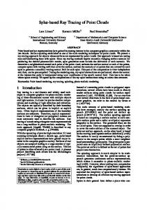
Figure 1: Comparison between a median split in a regular kd-tree (a) and in a Quantized kd-tree (b) in 1D. In (a) the split position is stored exactly, while in (b) quantization of the split offset leaves us with an uncertainty about the actual position. Classification of the points to child1 or child2 during construction of the tree is based on the real median position. Yet, while traversing, the exact position of the splitting point is no longer known. To account for this we let the two bounding intervals of the children overlap by the width of the quantization step. Note how the precision (i.e. the size of quantization intervals) is refined as we go from the parent to the children.
tree node will contain only a split plane position, from which the actual point positions will be inferred. Wald et al. [31] note that balancing may have a negative impact on performance. Fortunately, this loss is only significant for highly unevenly distributed point clouds (e.g. a caustics photon map in their case). However, most point-sampled models exhibit a fairly uniform distribution of points. Wald et al. report that for diffuse photon maps, which are closer to uniform, the performance loss due to using balancing is roughly 25%. This sacrifice will be necessary in order to achieve a compact memory footprint. 3.2
X2
Construction of the Quantized kd-tree
The quantized kd-tree is similar to the left-balanced kd-tree [14], but differs in several ways: • In each node we only store the split plane position d. d will be stored as offset d ∈ [0, 1) w.r.t. the current kd-tree node’s bounding box, rather than its absolute position in object space, using a short integer (bit string of length q) as opposed to a real number. In other words, d is quantized. However for the classification of the data to the left or right child the real median point is used, since we want to have a left-balanced tree. • Point positions are not stored alongside the kd-tree nodes. The actual coordinates of a point will be derived from the split plane positions in the tree. Since the splits d are actually offsets w.r.t. the current bounding box, the kd-tree recursively refines a point’s position as one goes deeper down the tree (see Figure 1). • Points are represented only by the leaf nodes, while in Jensen’s version, both leaf and inner nodes represents points. Since a point’s coordinates are defined recursively by the (quantized) split positions, points that would be stored higher up in the tree would be represented at a much lower precision. The quantization implies that the actual split plane position is no longer known exactly. However, we know that it has to lie on q an interval [ 2Dq , D+1 2q ], with D = ⌊2 d⌋ (see figure 1(b)). This “uncertainty” has 2 implications. First of all, it will affect how range queries are carried out (this will be discussed later). Second, it reduces the precision at which points are stored. Let us first look at how the points are stored.
Z2
Z
Y
Z5
Z4
Z3
Z
X
(a)
Z6
Z
Z7
Y
Z8
Z
(b)
Figure 2: (a) Due to the construction of the tree, the 4 left (right) leaf nodes retain the same X coordinate. This results in large errors. We work around this problem by storing each splitting plane’s (X, Y and Z) quantized value in the leaf nodes. (b) (upper)case: data (blue) is stored in last level. The entire red part of the tree is not used which yields to enormous compression overhead (b) (lower)case: data (blue) is stored in 2 last levels. The entire tree is used, no overhead.
3.3
Storing the points
At each inner node we save the quantized value of the splitting plane in one direction (X,Y or Z). If the same data is stored at the leaf level some information is lost. This is caused by the construction of the tree: since it takes 3 depth levels to update one coordinate component (see §3.2), two siblings differ only in the splitting plane coordinate component. This results in very large errors especially at the leaf nodes, since 4 leaf sibling will have the same X, Y or Z coordinate (see figure 2(a)). We work around these artifacts by storing each splitting plane’s (X, Y and Z) quantized value in the leaf nodes. If the point data is stored at each (leaf and inner) node of the tree, as Jensen proposed [14], the variation on the quantization error between points in the top and in the leaf nodes will be very high, leading to very large variations in quantization error. We therefore let the leaf nodes represent the actual input points, because the quantization error is the smallest in the deepest nodes of the kd-tree. If all N points are stored exclusively in the leaf level of the tree, a kd-tree with at least 2i leaf nodes is needed, where 2i−1 < N ≤ 2i . This kd-tree has i depth levels resulting in Ntot = 2i + 2i − 1 nodes. In a worst case situation, see figure 2(b)(upper), where N = 2i + 1, only half of the tree is used, but the entire tree is needed to use the heap properties of the kd-tree. A best case situation only occurs when N is a power of two, because then the efficiency of the tree is maximized. Clearly, when working with very large point sets it is unreasonable to expect this condition to be fulfilled. Therefore, we do not store the points exclusively in the leaf level. Instead, we store as many points N ′ as possible in the second last level, where N ′ = 2k with 2k ≤ N ′ < 2k + 1. The remainder R = N − N ′ is stored in a left balance way in the next level, see figure 2(b)(lower). Due to this construction R is always as small as possible R < 2k . The tree needs Ntot = 2k + 1 + R nodes which is equal to or better than the best case situation from the previous method. This left-balanced kd-tree always uses its full capacity, since all nodes are occupied. This way we have a very small variation in quantization error, at a reasonable cost. 3.4
Decoding and Querying the Quantized kd-tree
To decode a single point P, we start at the root of the tree which outlines the bounding box of all points. This is also the initial representation for P. We refine P’s representation by dividing the bounding box using its quantized splitting plane every time we go one level deeper in the tree, see figure 3. The traditional ray-tree traversal
P
P
P
P
xP = .38 + (.5 - .38)*6/8
Figure 3: Illustration of the decoding process in 1D. Let us consider a single point P with position xP . The actual position xP will be derived from the quantized median split positions in the tree, which define intervals where P resides (i.e., the extent of the kd-tree cell, indicated in gray). As we go down the tree, this interval gets refined by splitting the kd-tree nodes recursively. In the figure, median points that define the split are shaded in dark, while the stored quantized median position is depicted with a bold line. At the leaf level, the split plane position within the current interval defines the final position xP using the bounds of the corresponding interval.
and k-nearest neighbor spatial queries use the same traversal strategy, which makes this decoding scheme suitable for ray tracing. Due to the introduced quantization (see 3.2) the exact splitting plane position of a node is lost. During ray-tree traversal and spatial querying this quantization uncertainty introduces some problems. It is unclear which child will contain the query point if this is positioned near the real splitting plane, since the data is classified according to the real median point. To account for this, we do not split the bounding box at the quantized value, but let the two bounding boxes of the children overlap with one quantization step, as shown in Figure 1(b). Consequently, each quantized kd-tree inner node can, in contrast with the classical two region division, be classified into 3 regions: left, overlap and right. However, an inner node still has two children. Letting sibling kd-tree cells overlap is a conservative approach to maintain a consistent spatial data structure. In the same spirit, Mahovsky and Wyvill [20] quantize the vertices an axis-aligned bounding box, such that the quantized version encloses the original. The overlap incurs a performance penalty, since the elements contained within the enlarged cell will have a higher chance of becoming candidates in an intersection test or spatial query. In section 3.6 we will discuss a variable quantization scheme that alleviates this penalty. The kd-tree in our implementation serves 2 purposes. First of all, we use it to compute an estimate of the nearest ray-surface intersection point. Second, given this estimate, a spatial query is performed on the kd-tree in order to fetch a local neighborhood of points for the purpose of reconstructing the surface (see section 4). Ray-Tree Traversal Standard kd-trees are well known acceleration structures for ray tracing. A typical kd-tree traversal algorithm for ray tracing can be found in Wald’s thesis [29, chapter 7.2.2]. The algorithm takes as input a tree and a ray and recursively searches for the nearest primitive in the tree that is intersected by the ray. If the ray only hits the left or right region of the current inner node we can cull the subtree on the other side, and immediately proceed to the “touched” child. Our version of the algorithm is slightly different since we have to deal with three regions. If the ray hits the overlap region both children need to be processed. Spatial Queries Another benefit of standard kd-trees is their ability to perform fast spatial queries, such as k-nearest neighbor
queries. Since we want to perform spatial queries directly on the compressed data, we provide a way to execute k-nearest neighbor queries on the quantized kd-tree. The main idea is the same as in a regular k-nearest neighbor search on a kd-tree [7]. However there is one caveat. In the standard kd-tree k-nearest neighbor query for a point p, resulting in a set of k points K, it is always possible to skip one of the child nodes for examination if dist(p, splittingplane) > M with M = maxdist(p, pi ) for i : 1..k where p1 ..pk ∈ K. This means that the child node that does not contain the point p may be skipped if it is far enough away. In our case, we can not skip a child if p lies in or near the overlapping zone. 3.5
Precision
Let us analyze the precision of stored points in a 1D Quantized kd-tree. For simplicity, assume that the point cloud is uniformly distributed. At each new level, the quantization error will decrease by a factor of 1 at worst (i.e., no improvement) and a factor of D1 at best (see figure 1). On average, the error thus drops by a fac1 tor of α = D+1 2D each level. Note that 2 < α < 1. We eventually get a quantization step width (or precision) of α L × W , where L is the number of levels in the tree and W is the width of the scene’s bounding box. In 3D, L should be divided by 3, as a coordinate (e.g. X) is “refined” every 3 levels in a kd-tree. Similar to Botsch et al.’s octree coding scheme [8], the precision depends on the number of levels in the tree. In their case, preciL sion is increased faster, at a rate proportional to 12 , as opposed to L
α 3 . However, it is important to see that the quantization step width still decreases exponentially in our case, and therefore we get fairly good reconstruction, especially for large models. 3.6
Variable Quantization
Aggressive quantization has the advantage of yielding a high compression ratio, yet comes with a severe cost. First of all the introduced quantization error is rather high (e.g. 41.6 dB Peak Signal to Noise Ratio (PSNR) for David 28 M point model q = 2 ). Secondly, since the overlap regions higher up in the tree are big, there is a high probability that the overlap region is hit and both large subtrees need to be processed. This overhead results in slower tree traversal and spatial querying(see 3.4). We use a constant bitstring size per depth level, such that child nodes can still be addressed implicitly without pointers. All mentioned problems can be solved by simply increasing the accuracy of the first dm depth levels, using more bits. This barely affects the compression ratio since the last dtotal − dm depth levels, which still use a small bitstring, represent the largest part of the total data. We experimented with a simple heuristic to alter the bitstring length per level. We use 8 (or more) bits for the first ±80% of the levels, and q bits or less for the remaining levels. In table 1 one can see how the variable method outperforms the fixed one regarding the PSNR and the tree traversal and k-nearest neighbor querying overhead but still achieves good compression ratios. The q in table 1 only points to the fixed method. For each fixed method entry in the table we also provide a variable method entry with comparable compression ratio. 4
R AY T RACING P OINT S AMPLED M ODELS
In this section we give an example of how the quantized kd-tree can be used in the context of ray tracing large point clouds. The ray tracing algorithm we use is inspired by Wald and Seidel’s kdtree-based technique [32]. The main difference with their approach is that we fetch local k-neighborhoods on-the-fly, while Wald and
Seidel precompute and store them in the tree (albeit a significantly higher memory cost). Due to the surface model, per-point normals should also be stored alongside the positions in order to compute the intersection and shading. We use simple quantization based on Rusinkiewicz et al. [26] to compactly store them, at a cost of 12 bits per normal. However there are other, more computational expensive, ray surface intersection algorithms which do not need this normal information [2, 4]. We also describe an extension that allows for ray tracing with LOD using the Quantized kd-tree. Surface Model The surface is represented implicitly by a signed distance function φ ; the corresponding surface normals are defined by φ ’s normalized gradient. Shen et al. [28] proposed to construct φ by local blending of signed distance functions of the plane defined by a point and its normal.
φ (x) =
∑i w(kx − xi k)(x − xi )ni ∑i w(kx − xi k)
(1)
where xi and ni define the positions and normals of the point set surface, respectively. To allow an efficient computation of Equation 1, only points in the local neighborhood of x are considered significant. The interpolation function w is therefore chosen to be monotonically decreasing and compact. We choose a Gaussian weighting function similar to Kolluri et al. [16]: 2
− 2rσ 2
w(r) = e
(2)
Similar reconstruction methods are used by other authors [4, 1, 32]. Intersection Determination Let a ray R with anchor point Rorigin and direction Rdir be parameterized as r(t) = Rorigin +tRdir . Determining intersections boils down to tracking the nearest positive root of f = φ ◦ r. Root determination will consist of a global and a local step: root isolation and root refinement respectively [13]. The first step bounds the domain of f to the interval around the first root. The second step tracks the root in the interval. We make use of our kd-tree scheme for the root isolation step, by finding a candidate node that intersect the ray. The interval bounding the near and far intersection of the node’s bounding box isolates the root. We will locally reconstruct the signed distance function in this node in order to find the root. To this end, the kd-tree is queried to collect a local neighborhood of points, which will be used in evaluating equation 1. Finally, Newton’s method [25] returns the root of f = φ ◦ r. 4.1
Ray Tracing with LOD
When displaying large models (in the order of millions of points), several points may map to a single pixel on the screen, causing distracting aliasing problems. Moreover, these points can also require completely different data, this memory swapping/cache trashing can be very expensive. A simple approach to avoid these problems, is by using a multi-resolution representation (e.g. QSplat [26]). Such a representation contains different versions of the same scene, but re-sampled at different resolutions (e.g. from coarse to fine). By selecting the resolution that matches the size of the pixel, aliasing is reduced significantly. As an additional advantage of multiresolution rendering, usually a smaller fraction of the dataset is accessed, yielding an improved performance. The Quantized kd-tree implicitly represents the point cloud at multiple resolutions. As mentioned before, the split plane offsets can be used to reconstruct a position. By doing so higher up the hierarchy, one obtains a multi-resolution representation. Although the
(a)
(b)
(c)
Figure 4: The St. Matthew model (187M points) compressed to 5.2 bpp. The red square is a close up of the dotted red square. (a) is rendered using the multiresolution representation. (b) is rendered without using the multiresolution representation. Aliasing artefacts are visible in the magnified square. The rendering of (b) takes 9 times longer than (a). (c) is the visualization of the different levels of detail used to render (a).
reconstructed positions at inner nodes are actually the median split positions, rather than the average position of their children [26], for the purpose of display they do a reasonable job. See figure 4 for a demonstration. The only overhead that the multi-resolution representation incurs, is that additional 12-bit normal lookups have to be stored at the inner nodes. We can eliminate this overhead by using an other surface reconstruction algorithm that computes the normals on the fly as presented by Adamson et al. [2, 4]. 5
R ESULTS AND D ISCUSSION
We will empirically measure the performance in terms of precision, compression ratio and traversal/querying speed. The reconstruction quality of our compression scheme is measured in Peak Signal to Noise Ratio, PSNR. This is an engineering term for the ratio between the maximum possible power of a signal and the power of corrupting noise that affects the fidelity of its representation. Because many signals have a very wide dynamic range, PSNR is usually expressed in terms of the logarithmic decibel scale. To compare the overhead on the performance of the ray-tree traversal and spatial querying caused by the compression we provide in table 1 an entry of the uncompressed David model(consisting of 28M points). The table provides besides timings also the average number of nodes visited during a tree traversal and a k-nearest neighbor spatial query. As the table shows this introduced overhead is almost negligible for the variable bitlength compression method. Figure 5 gives an idea of the reconstruction quality 5(a) in function of compression ratio 5(b). Figure 6, shows the distribution of errors across the point cloud. Each plot is a histogram where the X axis represents the Real Mean Square Error (RMSE) and the Y axis the propability this error occurred. One can see that the introduced error is compact. Thus, no large variations on the error can occur. Figure 7 shows corresponding renderings of the plotted error histograms. One can see that the global reconstruction of the model is excellent for all compression ratios. Only when sharp or edgy features are magnified quantization errors become visible. In table 2 we present our compression results for several different models. For each model two results are presented, to show the compression and reconstruction properties . For smaller models the compression rate and reconstruction quality are not as competitive, due to the shallow tree depth, but are nevertheless reasonable. Note that the St Matthew model consists of 187M points and is divided into 12 blocks. Some blocks contain more than 35M
David 28M Fixed: q = 1 Variable Fixed: q = 2 Variable Fixed: q = 3 Variable Fixed: q = 4 Variable Uncompressed
bpp 3.5 3.6 7.19 5.6 8.6 8.6 14.3 15.5 96
PSNR(dB) 4.8 42.4 41.6 62.8 58.8 69.4 69.8 79.1 inf
Comp. Rat. 25.8 25.4 12.9 16.3 10.7 10.7 6.4 5.9 1
knn Nodes 33.5M (all) 26.6K 21K 256 2K 213 505 180 180
knn Overhead 1.8e5 147 116 1.42 11.1 1.18 2.8 1.0 1.0
Tree Trav. Nodes 33.5M(all) 8K 47K 880 5021 878 1846 875 830
Tree Trav. Overhead 4.0e4 9.64 56 1.06 6.05 1.06 2.22 1.05 1.0
Table 1: Results of our approach on the David model. The table’s columns show the bits per point (bpp), PSNR, compression ratio (Comp. Rat.), number of nodes visited during k-nearest neighbor (knn) querying, the overhead while performing a knn query due to the quantization (1.0 = no overhead), number of nodes visited during Ray-Tree Traversal and the associated overhead. The rows show different configurations of the quantization, including variable quantization.
(a)
(b)
(a)
(b)
(c)
(d)
Figure 5: (a) PSNR plot for different input quantizations (b) Compression Ratio for different input quantizations
Model St Matthew
#points 38M(187M)
TD 24
David
28M
24
Lucy
14M
23
Night
11M
23
Buddha
543K
19
Dragon
437K
18
bpp 5.2 13.2 5.6 15.5 5.3 12.2 5.6 13.7 4.8 14.6 4.6 15.5
PSNR(dB) 61.4 75.4 62.8 79.1 60.4 73.2 62.4 76.1 43.5 57.5 43.9 57.4
CR 17.5 7.2 16.3 5.9 17.2 7.5 16.3 7.0 19.3 6.3 20.0 5.9
Table 2: This table shows the compression and reconstruction properties for models with different size. TD: Quantized kd-tree depth, bpp: bits per point, CR: compression ratio.
points. Due to our current un optimized implementation time and memory considerations forced us to compress it one block at a time. However, it would be better for the compression ratio to compress St Matthew as one gigantic block of 187 M points, because more points could reuse the same data structure. We compared the rendering times of a compressed (890MB) and uncompressed3 (3.6 GB) St Matthew model on a PC with 2GB RAM memory. The uncompressed model required disk access during rendering, leading to a decreased performance. On average the rendering times dropped 2 to 4 times when compared with the compressed one, see figure 8. Decreases up to 15 times were measured when the camera was moved significantly. Thanks to the compression we were able to visualize several 3 The
normals were in both cases compressed to 12 bits per normal
Figure 6: (a)(b)(c)(d) RMSE histograms of the 28M David model. As the plot shows, the compression does not introduce large variations in the error.
models at the same time. Figure 9(a) shows the entire St Matthew statue together with David and Lucy, the total scene consists of 229M points. In order to create a massive scene we loaded two entire St Matthew statues, without instancing. The entire scene in figure 9(b) consists of 374M points. These scenes were rendered in 10 seconds at 512x512 resolution on one dual processor PC. As a proof of concept we compressed and ray traced several different large models. They are shown in figure 10. These models differ in complexity and geometric structure. 6
C ONCLUSION
We have presented a novel method to compress and display huge point clouds in combination with ray tracing. Our compression scheme based on a left balanced kd-tree, in order to avoid the cost of storing pointers. Compactness is achieved by quantizing the split plane positions. Our scheme is optimized for ray tracing pointsampled surfaces, and the decoding of the points can be carried out while traversing the tree. A valuable property of the Quantized kd-Tree is that both the geometric data and the acceleration data structure are compressed simultaneously. Our representation affords local decoding, such that spatial queries can be performed
(a)
(b)
(c)
(d)
Figure 10: (a) Night model (11M points) compressed to 5.6 bpp, PSNR 62.4dB, Comp. Rat. 16.4. The holes in this model are caused by the incomplete scanning, not by the quantization(b) Lucy model (14M points) compressed to 12.2 bpp, PSNR 73.25dB, Comp. Rat. 7.5. (c) Close up of St Matthew model (187M points) compressed to 5.2 bpp, PSNR 61.4dB, Comp. Rat. 17.5.(d) David model (28M points) compressed to 5.6 bpp, PSNR 62.8dB, Comp.Rat. 16.3.
(a)
(b)
(a)
(b)
Figure 8: In these figures we plotted the rendering times per frame in seconds for a prerecorded camera sequence. (a)The rendering times for a compressed St Matthew model. The compressed model fitted in the main memory and resulted in a constant frame rate. (b) The same camera sequence but rendered with an uncompressed St Matthews model. The uncompressed model did not fit into the main memory and required disk access during rendering, leading to a decreased performance. The peaks are caused by significant camera movements, in these cases large parts of the model needed to be loaded from disk into main memory.
(c)
(d)
Figure 7: These figures are a visualization of the 28M David corresponding to the error histograms shown in figure 6. One can see that the global reconstruction is excellent, and the quantization artefacts only occur when sharp features are magnified.(a) 5.6 bpp, PSNR: 62.8 dB (b) 8.6 bpp, PSNR: 69.4 dB (c) 15.5 bpp, PSNR: 79.1 dB (d) Uncompressed model : ground truth 96 bpp, PSNR: inf
without decompressing the full dataset. In addition, it provides a multiresolution representation of the point cloud, which improves performance and image quality. So far we have only considered only the compression of 3D positions. However, points may have other attributes such as colors and normals. In future work we wish to tie in the compression of these attributes with the positions stored in the Quantized kd-tree. In addition, we would like to combine our representation with a parallelized ray tracing algorithm [29], in order to achieve interactive performance. Acknowledgements We would like to thank Yeuhi Abe, Johan Claes, Fredo Durand, Jan Fransens, Mark Gerrits and Jonathan
Ragan-Kelley for their helpful comments, and Cedric Vanaken for his assistance in writing this paper. We acknowledge the Stanford Graphics Group for making their datasets available. Finally, we would like to thank the anonymous reviewers for their constructive comments. Part of the research at the Expertise Centre for Digital Media is funded by the ERDF (European Regional Development Fund), the Flemish Government and the Flemish Interdisciplinary institute for Broadband Technology (IBBT). Tom Mertens acknowledges a research fellowship from the Belgian American Educational Foundation.
R EFERENCES [1] Bart Adams, Richard Keiser, Mark Pauly, Leonidas J. Guibas, Markus Gross, and Philip Dutre. Efficient Raytracing of Deforming PointSampled Surfaces. volume 24, pages 677–684, 2005. [2] Anders Adamson and Marc Alexa. Approximating and intersecting surfaces from points. In SGP ’03: Proceedings of the 2003 Eurographics/ACM SIGGRAPH symposium on Geometry processing,
[21]
[22]
[23] (a)
(b)
Figure 9: (a) Scene of 229M points rendered in 9 sec on one PC (512x512) (b) Scene of 2 St Matthew statues without instancing consisting of 374M points rendered in +/-10 sec on one PC(512x512)
[24]
[25]
[3]
[4]
[5] [6] [7] [8]
[9]
[10]
[11]
[12] [13] [14] [15] [16]
[17]
[18] [19]
[20]
pages 230–239, Aire-la-Ville, Switzerland, Switzerland, 2003. Eurographics Association. Anders Adamson and Marc Alexa. Ray tracing point set surfaces. In SMI ’03: Proceedings of the Shape Modeling International 2003, page 298, Washington, DC, USA, 2003. IEEE Computer Society. Anders Adamson and Marc Alexa. Approximating bounded, nonorientable surfaces from points. In Proceedings of Shape Modeling and Applications, pages 243–252, 2004. Timo Aila. Efficient Algorithms for Occlusion Culling and Shadows. PhD thesis, Helsinki University of Technology, 2005. Pierre Alliez and Craig Gotsman. Recent Advances in Compression of 3D Meshes. 2005. J.L. Bentley. Multidimensional binary search trees used for associative searching. CACM, 18(9):509–517, September 1975. Mario Botsch, Andreas Wiratanaya, and Leif Kobbelt. Efficient high quality rendering of point sampled geometry. In EGRW ’02: Proceedings of the 13th Eurographics workshop on Rendering, pages 53–64, Aire-la-Ville, Switzerland, 2002. Eurographics Association. Carsten Dachsbacher, Christian Vogelgsang, and Marc Stamminger. Sequential point trees. ACM Transactions on Graphics (Proceedings of ACM SIGGRAPH 2003), 22(3):657 – 662, 2003. Shachar Fleishman, Daniel Cohen-Or, Marc Alexa, and Claudio T. Silva. Progressive point set surfaces. ACM Trans. Graph., 22(4):997– 1011, 2003. Pierre-Marie Gandoin and Olivier Devillers. Progressive lossless compression of arbitrary simplicial complexes. In SIGGRAPH ’02: Proceedings of the 29th annual conference on Computer graphics and interactive techniques, pages 372–379, New York, NY, USA, 2002. ACM Press. Stefan Gumhold, Zachi Karni, Martin Isenburg, and Hans-Peter Seidel. Predictive point-cloud compression. In Siggraph Sketches, 2005. John C. Hart. Ray tracing implicit surfaces. In Siggraph ’93 course notes: Designm Visualisation and Animatin of implicit Surfaces, 1993. Henrik Wann Jensen. Realistic image synthesis using photon mapping. A. K. Peters, Ltd., Natick, MA, USA, 2001. A. Kalaiah and A. Varshney. Statistical point geometry. In Eurographics Symposium on Geometry Processing, pages 113–122, June 2003. Ravikrishna Kolluri. Provably good moving least squares. In Proceedings of ACM-SIAM Symposium on Discrete Algorithms, pages 1008– 1018, August 2005. Jens Kr¨uger, Jens Schneider, and R¨udiger Westermann. Duodecim - a structure for point scan compression and rendering. In Proceedings of the Symposium on Point-Based Graphics 2005, 2005. David Levin. Mesh-independent surface interpolation. In Geometric Modeling for Scientific Visualization, pages 37–49, 2003. Marc Levoy and Turner Whitted. The use of points as a display primitive. Technical Report TR 85-022, University of North Carolina at Chapel Hill, 1985. Jeffrey Mahovsky and Brian Wyvill. Memory conserving bounding
[26]
[27]
[28]
[29] [30]
[31]
[32]
[33] [34]
[35] [36]
volume hierarchies with coherent ray tracing. Computer Graphics Forum, 25(2):173–182, 2006. Bruce Merry, Patrick Marais, and James Gain. Compression of dense and regular point clouds. In AFRIGRAPH 2006: Proceedings of the 4th international conference on Computer graphics, virtual reality, visualisation and interaction in Africa, pages 15–20, New York, NY, USA, 2006. ACM Press. T. Ochotta and D. Saupe. Compression of point-based 3d models by shape-adaptive wavelet coding of multi-height fields. Proceedings Symposium on Point-Based Graphics, pages 103–112, 2004. Hanspeter Pfister, Matthias Zwicker, Jeroen van Baar, and Markus Gross. Surfels: surface elements as rendering primitives. In SIGGRAPH ’00, pages 335–342, New York, NY, USA, 2000. ACM Press/Addison-Wesley Publishing Co. Matt Pharr, Craig Kolb, Reid Gershbein, and Pat Hanrahan. Rendering complex scenes with memory-coherent ray tracing. In SIGGRAPH ’97: Proceedings of the 24th annual conference on Computer graphics and interactive techniques, pages 101–108, New York, NY, USA, 1997. ACM Press/Addison-Wesley Publishing Co. William H. Press, Brian P. Flannery, Saul A. Teukolsky, and William T. Vetterling. Numerical Recipes. Cambridge University Press, 2nd edition, 1992. Szymon Rusinkiewicz and Marc Levoy. QSplat: A multiresolution point rendering system for large meshes. In Siggraph 2000 Proceedings, pages 343–352, 2000. Gernot Schaufler and Henrik Wann Jensen. Ray tracing point sampled geometry. In Proceedings of the Eurographics Workshop on Rendering Techniques 2000, pages 319–328, London, UK, 2000. SpringerVerlag. Chen Shen, James F. O’Brien, and Jonathan R. Shewchuk. Interpolating and approximating implicit surfaces from polygon soup. ACM Transactions on Graphics, 23(3):896–904, August 2004. Ingo Wald. Realtime Ray Tracing and Interactive Global Illumination. PhD thesis, Computer Graphics Group, Saarland University, 2004. Ingo Wald, Andreas Dietrich, and Philipp Slusallek. An interactive out-of-core rendering framework for visualizing massively complex models. In Alexander Keller and Henrik Wann Jensen, editors, Rendering Techniques 2004 : Eurographics Symposium on Rendering, pages 81–92, Norrkoeping, Sweden, 2004. Eurographics. Ingo Wald, Johannes G¨unther, and Philipp Slusallek. Balancing Considered Harmful – Faster Photon Mapping using the Voxel Volume Heuristic. Computer Graphics Forum, 22(3):595–603, 2004. (Proceedings of Eurographics). Ingo Wald and Hans-Peter Seidel. Interactive Ray Tracing of Point Based Models. In Proceedings of 2005 Symposium on Point Based Graphics, pages 9–16, 2005. Michael Wand and Wolfgang Straßer. Multi-resolution point-sample raytracing. In Proceedings of Graphics Interface, 2003. M. Waschb¨uch, M. Gross, F. Eberhard, E. Lamboray, and S. W¨urmlin. Progressive compression of point-sampled models. In Eurographics Symposium on Point-Based Graphics, pages 95–102, 2004. Turner Whitted. An improved illumination model for shaded display. Commun. ACM, 23(6):343–349, 1980. Matthias Zwicker, Hanspeter Pfister, Jeroen van Baar, and Markus Gross. Surface splatting. In SIGGRAPH ’01, pages 371–378, New York, NY, USA, 2001. ACM Press.