Spread Spectrum Watermarking Security - CiteSeerX

IEEE TRANSACTIONS ON INFORMATION FORENSICS AND SECURITY

1

Spread Spectrum Watermarking Security Luis Pérez-Freire† and Fernando Pérez-González, Member, IEEE

Abstract This paper presents both theoretical and practical analyses of the security offered by watermarking and data hiding methods based on spread spectrum. In this context, security is understood as the difficulty of estimating the secret parameters of the embedding function based on the observation of watermarked signals. On the theoretical side, the security is quantified from an information-theoretic point of view by means of the equivocation about the secret parameters. The main results reveal fundamental limits and bounds on security and provide insight into other properties, such as the impact of the embedding parameters, and the tradeoff between robustness and security. On the practical side, workable estimators of the secret parameters are proposed and theoretically analyzed for a variety of scenarios, providing a comparison with previous approaches, and showing that the security of many schemes used in practice can be fairly low.

Index Terms Spread spectrum, watermarking security, information leakage, equivocation, parameter estimation, PCA, ICA, Constant Modulus

EDICS Category: WAT-SSPM, WAT-THEO, WAT-OTHA I. I NTRODUCTION The notion of security in watermarking has started to being considered several years ago [1], [2], although the first attempt at providing a mathematical framework for assessing watermarking security was [3], which gave rise to other related works as [4] and [5]. The present paper considers the security of spread spectrum methods for watermarking and data hiding following the same guidelines as in the aforementioned works. The fundamentals of this approach to security assessment can be found in [4], where the attacks to the security of watermarking and data hiding methods are defined as those aimed at gaining knowledge about the secret parameters of the system. The key assumptions are that the watermarker owns a secret key that he/she repeatedly uses to watermark contents, and an attacker is able to gather several signals (observations) that were watermarked with the same secret key; if the attacker manages The authors are with the Signal Theory and Communications Dept., ETSI Telecommunications, University of Vigo, 36310 Vigo, Spain (e-mail: {lpfreire,fperez}@gts.tsc.uvigo.es) † Luis Pérez-Freire holds a temporary postdoctoral research position in the Security Labs of Thomson R&D, France. This work was supported in part by Xunta de Galicia under Projects 07TIC012322PR (FACTICA), 2007/149 (REGACOM), 2006/150 (“Consolidation of Research Units”), and by the Spanish Ministry of Science and Innovation under projects COMONSENS (ref. CSD200800010) of the CONSOLIDER-INGENIO 2010 Program and SPROACTIVE (ref. TEC2007-68094-C02-01/TCM). October 6, 2008

DRAFT

2


to estimate this secret key from the observations at hand, then he/she has completely “broken” the watermarking system [3],[6]. An additional assumption is that all parameters of the watermarking scheme are known (except the secret key), according to Kerckhoffs’ principle; hence, the attacker is only interested in disclosing the secret key. The information about the key provided by the observations is quantified by means of the Shannon’s mutual information, and the remaining uncertainty or “equivocation” about the key is measured by the differential entropy of the key conditioned on the observations, which can be related to the lowest attainable error in the estimation of the secret key. The number of observations needed to achieve a certain estimation accuracy can be regarded to as the “security level” of the watermarking scheme. This approach has been utilized in [6] and [7] for analyzing the security of lattice DCDM methods, and it is used here for developing a complete security analysis of spread spectrum methods, i.e., those methods that perform watermark embedding in a secret subspace by modulating a “secret carrier” with the symbols to be embedded. Specifically, three well-known data hiding methods are considered: additive Spread Spectrum [8], attenuated Spread Spectrum [9], and Improved Spread Spectrum [10]. Two different scenarios for security assessment are considered, according to the classification given in [3]: 1) Known Message Attack (KMA): the attacker is assumed to have access to watermarked signals and the messages embedded in each of those signals. This scenario constitutes the basis for the study of more involved scenarios and provides the main insight into the security problem (influence of the embedding parameters). It is also useful for the study of security in some watermark detection scenarios. 2) Watermarked Only Attack (WOA): the only information available to the attacker are the watermarked signals, without any knowledge of the embedded messages. As such, WOA models most of the data hiding scenarios of practical interest. The reader must be aware that the security of spread spectrum watermarking has been first addressed in [3]. An obvious difference between the present paper and [3] is that we resort to the Shannon’s equivocation instead of the Fisher information for performing the theoretical analysis. Further contributions of the present paper, which have not been previously addressed by other authors, are the following: the evaluation of the security in asymptotic conditions, the evaluation of the tradeoff robustness-security in the considered embedding functions, the derivation of bounds on the estimation performance, the theoretical analysis of the estimators proposed in [3], the proposal of new estimators, and their application to practical scenarios. Some of these contributions have been partially presented in [11]. Spread spectrum methods continue to be widely used, as many embedding functions existing nowadays are based on spreading. Thus, the analysis presented in this paper is expected to provide useful insights in the identification of security weaknesses of current spread spectrum schemes and the design of improved ones. In this regard, we want to remark that spread-spectrum-based embedding functions with improved security features have already been proposed by other authors in [12]. One of these embedding functions (Natural Watermarking) achieves perfect secrecy for Gaussian hosts. The other one (Circular Watermarking) is strongly related to the ISS embedding function analyzed in this paper, and it is briefly addressed in Section VII-A2 from a practical point of view. Another interesting contribution from [12] is the proposal of a general formulation for clarifying the different degrees of security existent in data hiding. Based on Kerckhoffs’ principle, the following classification of data hiding schemes (in increasing order of security) DRAFT

October 6, 2008

´ ´ ´ PEREZ-FREIRE AND PEREZ-GONZ ALEZ: SPREAD SPECTRUM WATERMARKING SECURITY

3

is proposed: insecure, key secure, subspace secure, and stegosecure. These security classes are related to the degree of concealment of the secret keys. All the methods analyzed in the present paper pertain to the category of insecure, with the exception of Circular Watermarking, which is key secure. The practical estimators used in [12] are the same as those used in [3]. The remaining of this paper is organized as follows. In Section II, the problem is formalized, introducing the working assumptions and the notation. Section III studies the security of the classical spread spectrum embedding function, whereas Section IV addresses the security when host rejection is considered. In Section V, we provide bounds for the estimation of the spreading vector based on the information-theoretic analysis of the previous sections. In Section VI, practical methods for estimating the secret key are proposed and analyzed, and Section VII shows experimental results obtained on real images, also briefly discussing the extension of the proposed estimators to other scenarios. In Section VIII we consider the links, in terms of security, between the methods studied here and other methods that are strongly related to the spread spectrum formulation followed in this paper. Finally, the conclusions are summarized in Section IX. II. F ORMAL

PROBLEM STATEMENT AND NOTATION

In this section, the problem of watermarking security is formalized. Hereinafter, boldface letters denote column vectors, whereas italicized letters denote scalar variables. The considered scenario is the following: the secret key of a certain user is reutilized No times for watermarking a set of host signals {xi ∈ Rn×1 , i = 1, . . . , No }, where xi,j is the j th component of the ith host vector. These vectors xi are usually obtained through some partition of the digital item (image, audio signal, etc.) to be watermarked. The secret key is a n-dimensional vector s that parameterizes the embedding function, and it is usually termed “secret carrier” or “spreading vector” (we will use both terms without distinction). For the family of methods considered in this paper, the embedding function can be written as yi = xi + (−1)mi s + Ψ(xi , s) = xi + wi , i = 1, . . . , No ,

(1)

where mi ∈ M = {0, 1} denotes the embedded message that modulates s, and the function Ψ : Rn×1 ×Rn×1 → Rn×1 is used for host-rejection purposes. The resulting embedding rate of the scheme is R , log(2)/n. We will consider that the objective of the attacker is to obtain an estimate of s using the information contained in the sequence of observations {oi , i = 1, . . . , No }, where oi = [yTi , mi ]T in the KMA case,1 and oi = yi in the WOA case. The signals involved in the theoretical security analysis will be modeled as random variables, which will be denoted by capital letters. Instantiations of these random variables will be denoted by lowercase letters as in (1). For the theoretical analysis, the host signals {Xi , i = 1, . . . , No } will be assumed to be i.i.d. and Gaussian-distributed

2 I ), where I denotes the identity matrix of size n × n. Furthermore, the X are with zero mean: Xi ∼ N (0, σX n n i

assumed to be mutually independent. The messages {Mi , i = 1, . . . , No } embedded in different observations are assumed to be mutually independent and equiprobable in M = {0, 1}. As for the spreading vector, it is assumed to

be Gaussian-distributed and i.i.d, S ∼ N (0, σS2 In ). The motivation for this choice is twofold: 1) on one hand, the 1

The notation [a, b] indicates concatenation of the row vectors a and b.

October 6, 2008

DRAFT

4


Gaussian distribution for S is a long-standing assumption [8] that has been frequently recalled in later theoretical analysis (also for mathematical simplicity); 2) on the other hand, for a given embedding distortion, the Gaussian distribution maximizes the a priori entropy of S, which is desirable from the security standpoint. The information about S provided by the observations is frequently referred to as “information leakage”. This information will be quantified in an information-theoretic manner by means of the mutual information between S and the observations [13], which is denoted by I(O1 , . . . , ONo ; S). The remaining uncertainty about S, given No observations, will be represented by means of the “equivocation” or “residual entropy”, defined as h(S|O1 , . . . , ONo ), where h(A) denotes the differential entropy of the continuous random variable A [13]. For a discrete random variable B , the entropy will be denoted by H(B). Throughout this paper, all the entropies and mutual informations will be

expressed in natural units. Notice that the a priori uncertainty about S is given by h(S), and that the equivocation is a decreasing function of No . The number of observations (No ) needed to achieve a certain value of the equivocation is regarded to as the security level of the watemarking method. For providing a fair comparison between the security level of the different methods, they will be studied under the same conditions of embedding distortion. The embedding distortion per dimension is defined as Dw , n1 E[||Wi ||2 ]. Thus, Dw quantifies the power of the watermark. Furthermore, we define the Document to Watermark Ratio (DWR) for quantifying the relative powers between the host and the watermark: DWR , 10 log10

1 2 n E[||Xi || ]

Dw

= 10 log10 ξ,

2 /D , the operator E [·] denotes mathematical expectation, and ||x||2 , where ξ , σX w

Euclidean norm of x.

2 i xi

P

denotes the squared

2 I ), Other notational conventions are the following: Γ(z) denotes the complete Gamma function. If X ∼ N (0, σX n

then T , ||X||2 follows a Chi-squared distribution with n degrees of freedom, which is denoted as χ2 (n, σX ). If 2 I ), then T ′ , ||X||2 follows a noncentral Chi-squared, denoted by χ′2 (n, v, σ ). The probability X ∼ N (v, σX n X

density function (pdf) of a continuous random variable A is denoted by f (a). The transpose of a vector x is denoted ˆ. by xT . The estimate of the vector x is denoted by x

III. A DDITIVE S PREAD S PECTRUM ( ADD -SS) Binary add-SS, as proposed by Cox et al. [8], is the most popular and widely studied watermarking method. No host rejection is performed, so the embedding function is simply given by Yi = Xi + (−1)Mi S, for i = 1, . . . , No .

(2)

The embedding distortion results in Dw = σS2 . The security level for KMA and WOA scenarios is addressed below. A. KMA scenario Under the assumptions made in Section II, the KMA scenario can be seen as a simple additive Gaussian channel. Although this scenario was already considered in [4], a simple, alternative derivation is given in this paper for the sake of completeness. Furthermore, this derivation introduces some results that will be used later on. Let us denote DRAFT

October 6, 2008


5

equivocation per dimension (nats) 1.5 1 0.5 0 −0.5 −1 −1.5 −2 15

20

25

DWR (dB)

Fig. 1.

30

6000

4000 No

2000

0

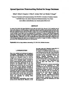
Equivocation per dimension for add-SS in the KMA scenario.

¯ N the random variable S conditioned on No observations. From the embedding function of add-SS, it follows by S o ¯ N are all mutually independent and Gaussian-distributed [14]. Given a that the components {S¯i , i = 1, . . . , n}, of S o ¯ N ∼ N (v, σ 2¯ In ), with particular realization {Y1 = y1 , . . . , YNo = yNo , M1 = m1 , . . . , MNo = mNo }, we have S o SN o

vi = σS2¯N

o

=

σS2 T (i) 2 µ y , No σS2 + σX 2 σ2 σX S 2 , No σS2 + σX

i = 1, . . . , n,

(3) (4)

¯ N is i.i.d. Gaussian, its entropy is given where µ , [(−1)m1 , . . . , (−1)mNo ]T , and y(i) , [y1,i , . . . , yNo ,i ]T . Since S o ¯N ) = by h(S o

n 2

log(2πeσS2¯N ), which does not depend on the particular realization of the observations. Hence, we o

can conclude that the equivocation per dimension is σS2 1 1 h(S|Y1 , . . . , YNo , M1 , . . . , MNo )add-SS = log 2πe . n 2 1 + No · ξ −1

(5)

Now, it is straightforward to see that the information leakage per dimension reads as 1 1 I(Y1 , . . . , YNo ; S|M1 , . . . , MNo )add-SS = log 1 + No · ξ −1 . n 2

(6)

The information leakage (equivocation) is concave (convex) and strictly increasing (decreasing) with No , and its increasing (decreasing) rate is dependent on the DWR. Although (5) depends on the value of σS2 , for large No we 2 /N , as can be seen in Fig. 1. Notice that both (5) have n1 h(S|Y1 , . . . , YNo , M1 , . . . , MNo )add-SS ≈ 12 log 2πeσX o and (6) are independent of n, meaning that the information leakage about each dimension is independent of the total

number of dimensions. In other words, the difficulty of estimating each component of S does not depend on its total length when the embedded messages are a priori known. B. WOA scenario The WOA scenario can be seen as an additive Gaussian channel with an unknown scaling factor which, according to the binary transmission scheme given in Eq. (2) and the assumptions stated in Section II, takes values ±1 equiprobably October 6, 2008

DRAFT

6


in each channel use. In this case, an exact expression for the information leakage cannot be obtained, so we derive upper and lower bounds. Following an approach similar to [7], by resorting to the chain rule for mutual informations [13], the information leakage is rewritten as I(Y1 , . . . , YNo ; S)add-SS = I(Y1 , . . . , YNo ; S, M1 , . . . , MNo )add-SS − I(Y1 , . . . , YNo ; M1 , . . . , MNo |S)add-SS = I(Y1 , . . . , YNo ; S|M1 , . . . , MNo )add-SS + I(Y1 , . . . , YNo ; M1 , . . . , MNo )add-SS − I(Y1 , . . . , YNo ; M1 , . . . , MNo |S)add-SS .

(7)

The first term of Eq. (7) has been already calculated in (6). The second and third terms of (7) represent the amount of information that can be learned by an attacker and by a fair user, respectively, about the sequence of embedded messages. These quantities are studied in Appendix A, resulting in the following upper and lower bounds to the information leakage per dimension: 1 I(Y1 , . . . , YNo ; S)add-SS ≤ n −

No 1 ¯ N + (−1)MNo VN ; MN |VN ) log 1 + No · ξ −1 + I(X o o o o 2 n No I(X1 + (−1)M1 S; M1 |S), for No ≥ 2, n

(8)

and 1 I(Y1 , . . . , YNo ; S)add-SS ≥ n −

N

o 1X 1 −1 ¯ i + (−1)Mi Vi ; Mi |Vi ) I(X log 1 + No · ξ + 2 n

i=2

No I(X1 + (−1)M1 S; M1 |S), for No ≥ 2. n

(9) 4

S ¯ i ∼ N (0, (σ 2 + σ 2¯ )In ), with σ 2¯ given by (4), and Vi ∼ N (0, (i−1)σ In the expressions (8) and (9), X X (i−1)σ 2 +σ 2 In ). Si−1 Si−1 S

X

The second and third terms of (8) and (9) must be computed by taking into account that 1 2 kSk2 , I(X1 + (−1)M1 S; M1 |S)add-SS = E h((−1)M1 ||S||2 + XT1 S|S = s) − E log 2πeσX 2

where the expectation is taken over S. Notice that the above upper and lower bounds differ only in their second term. Nevertheless, they cannot be given in closed-form, so numerical integration (on a scalar domain) is needed. This integration is straightforward because, under the i.i.d. Gaussian assumption for S, ||S||2 follows a Chi-square

distribution χ2 (n, σS ). A comparison between the information leakage (per dimension) in KMA and WOA scenarios

is shown in Fig. 2: •

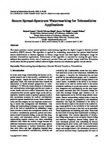
Fig. 2(a) shows that, when the parameter n is fixed, decreasing the DWR increases the information leakage in the KMA scenario (recall Eq. (6)), and simultaneously reduces the gap between KMA and WOA.

•

Fig. 2(b) shows the effect of varying the length of the spreading vector, n, when the DWR is fixed. In this case, we can see that the information leakage of the KMA scenario is approached as n is increased. Thus, the security level of the WOA scenario is strongly dependent on the value of n, contrarily to the KMA scenario.

The asymptotic behavior of the information leakage is formalized below. First, let us define the “loss function” as δ(No )add-SS , I(Y1 , . . . , YNo ; S|M1 , . . . , MNo )add-SS − I(Y1 , . . . , YNo ; S)add-SS = h(Y1 , . . . , YNo ; M1 , . . . , MNo |S)add-SS − h(Y 1 , . . . , YNo ; M1 , . . . , MNo )add-SS . DRAFT

(10)

October 6, 2008


2

0.8 KMA upper bound, WOA lower bound, WOA

0.7

DWR=12 dB

1.5

DWR=20 dB 1

0.5

DWR=30 dB

mutual information per dimension

mutual information per dimension

2.5

KMA upper bound, WOA lower bound, WOA

200

400

600

800

1000

n=2000

0.6 0.5 n=800

0.4 0.3 0.2 n=100

0.1 0 0

7

0 0

200

No

400

600

800

1000

No

(a) n = 100

(b) DWR = 25 dB

Fig. 2. Comparison between the information leakage in KMA and WOA scenarios for add-SS. Figures 2(a) and 2(b) show the effect of varying the DWR and n, respectively.

The loss function represents the information about S that is lost due to the a priori ignorance of the embedded messages, and it is non-negative for all No . Theorem 1: The loss function for add-SS in the WOA scenario can be upper bounded as n ! No X τi 2 H δ(No )add-SS ≤ log(2) + , 2

(11)

i=2

where τi =

2 + σ4 iσS2 σX X 4 2 + σ4 , (i − 1)σS + iσS2 σX X

and H(·) denotes the binary entropy function. The right hand side of (11) is decreasing with n and DWR−1 , and the following asymptotic properties hold: lim δ(No )add-SS ≤ log(2). DWR→−∞ 2) For fixed DWR, lim δ(No )add-SS ≤ log(2).

1) For fixed n,

n→∞

Proof: See Appendix B. Theorem 1 basically states that the ignorance of the embedded messages does not affect the difficulty of estimating S if either the DWR or the embedding rate R (recall that R = log(2)/n) are small enough. Although the first case is

of virtually null relevance in practice, the second case is of major importance for practical applications. When high robustness is sought, the watermark is usually embedded at very low rates that allow to recover the message with low complexity. In such case a few observations suffice to obtain an estimate of S that in turn allows accurate recovery of the embedded message. Nevertheless, it is important to point out, as realized before in [3] (by means of blind source separation theoretic arguments), that the penalty to pay for not knowing the messages Mi comes in the form of an ambiguity in the sign of S, independently of n and of the DWR. An alternative way for proving this ambiguity is to show that the a posteriori probability of the spreading vector in the WOA scenario is independent of its sign. One October 6, 2008

DRAFT

8


can easily check that f (s0 |Yi = yi ) =

f (yi |S = s0 )f (s0 ) f (yi |S = −s0 )f (−s0 ) = = f (−s0 |Yi = yi ) ∀ s0 ∈ Rn , f (yi ) f (yi )

(12)

so the sign ambiguity becomes patent. Notice that (12) holds regardless of the statistical distribution of the host, but it is needed that S is circularly symmetric. In the information-theoretic analysis, the sign ambiguity is reflected in the factor log(2) shown in Theorem 1. The sign ambiguity is irreducible without a priori knowledge of the embedded messages. For instance, in the particular case where all Mi = M in the No observations, the sign ambiguity still exists, and it cannot be undone unless one of the Mi is known by the attacker. In any case, the sign ambiguity does not prevent from estimating the one-dimensional subspace spanned by s, a feature that will be exploited by practical estimators in Section VI. IV. S PREAD S PECTRUM

WITH HOST REJECTION

After studying the security properties of add-SS, the influence of the host rejection mechanisms in the security level is addressed in this section. Two particular methods are studied: “attenuated spread spectrum” [9] and “improved spread spectrum” [10].

A. Attenuated Spread Spectrum (γ -SS) The attenuated spread spectrum technique proposed in [9] consists in attenuating the host prior to embedding, in order to optimize the power transmission subject to an MSE distortion constraint (the embedding distortion). The embedding function is as follows: Yi = (1 − γ) · Xi + (−1)Mi · S, for i = 1, . . . , No ,

(13)

2 +σ 2 . where 0 ≤ γ ≤ 1 is a host-rejection parameter. The embedding distortion of this scheme is given by Dw = γ 2 σX S

We will refer to this technique in the following as γ -SS. The parameter γ can be adjusted so as to optimize some performance measure, usually the error probability. Thus, the performance (in terms of robustness) of γ -SS is at least as good as that of add-SS, as the latter is just a particular case of γ -SS for γ = 0. However, its security level can be shown to be always worse than that of add-SS for the same values of DWR and n. In order to provide a fair 2 ξ −1 − γ 2 so as to get D = σ 2 as in add-SS. Note comparison between both schemes, we impose that σS2 = σX w S 1

that this condition restricts the value of γ to the interval 0 ≤ γ ≤ ξ − 2 , i.e. in practical scenarios (with low embedding distortion) γ takes values close to 0. It is easy to see that the results obtained for add-SS can be straightforwardly 2 ξ −1 − γ 2 and σ 2 by (1 − γ)2 σ 2 in the corresponding expressions. The adapted to γ -SS replacing σS2 by σX X X equivocation for the KMA scenario, for instance, results in

2 (ξ −1 − γ 2 )(1 − γ)2 σX 1 1 h(S|Y1 , . . . , YNo , M1 , . . . , MNo )γ -SS = log 2πe . n 2 (1 − γ)2 + No (ξ −1 − γ 2 )

(14)

The expression above can be shown to be monotonically decreasing with γ . The results for add-SS WOA can be easily generalized as well to γ -SS. The most interesting consequence of introducing the parameter γ is the existence of a tradeoff between robustness and security. This tradeoff is illustrated in Fig. 3(a), which shows the plot of the DRAFT

October 6, 2008


9

−3

x 10

0.2

1.6

0

1.4

1 0.8

1

1

equivocation per dimension

1.2 I( Y ;M | S)/n

γ = 0.01 γ = 0.05 add−SS (γ=0)

0.6 0.4

−0.2 −0.4 −0.6 −0.8

0.2 −1

0 0 500 n

1000

1

0.5

0

I( Y ; S|M )/n 1

1

1.5 x 10

−3

−1.2 0

200

400

600

800

1000

N

o

(a)

(b) 1

Fig. 3. γ-SS for KMA scenario and DWR = 25 dB. Tradeoff robustness-security as a result of varying γ in the interval [0, ξ − 2 ], for No = 1 (a) and equivocation per dimension (b).

information leakage for No = 1 (in the KMA scenario) vs. the achievable rate for a fair user. The latter can be computed by numerical integration by taking into account that 1 2 kSk2 . I((1 − γ)X1 + (−1)M1 S; M1 |S)γ -SS = E h((−1)M1 ||S||2 + (1 − γ)XT1 S|S) − E log 2πe(1 − γ)2 σX 2

Fig. 3(a) basically shows that increasing the achievable rate for fair users will provide more information for attackers interested in estimating S. As can be seen, the tradeoff is also dependent of n, since this parameter affects the achievable rate. Fig. 3(b) shows the equivocation per dimension in the KMA scenario for several values of the parameter γ , evidencing the degradation of the security level as the host rejection is increased. B. Improved Spread Spectrum (ISS) ISS [10] is the result of introducing a host-interference-rejection mechanism in add-SS, fundamentally different from γ -SS in that ISS attenuates the host only in the direction of embedding, thus saving in embedding distortion and improving the performance of the latter in terms of robustness. We will consider the linear version of ISS, whose embedding function is as follows: Yi = Xi + (−1)Mi νS − λ

XTi S S, for i = 1, . . . , No , ||S||2

(15)

where 0 ≤ λ ≤ 1 is the host-rejection parameter, and ν is a parameter for fixing the embedding distortion. The embedding distortion in ISS can be computed as follows. For the i-th observation and a particular s we have "

# T 2

X s i 2 M 2 2 2 2 i

E[||Wi || |S = s] = E

(−1) ν − λ ||s||2 s = ν ||s|| + λ σX .

(16)

2

2 , which is the same result as Finally, for a zero-mean Gaussian spreading vector, Dw = n1 E[||Wi ||2 ] = ν 2 σS2 + λn σX

for a spreading vector with constant norm equal to nσS2 (the case originally considered in [10]). For a fair comparison

with add-SS, the embedding distortion is fixed to Dw = σS2 , as proposed by Malvar and Florêncio [10]. This imposes 1 λ2 ξ 2 . (17) ν = 1− n October 6, 2008

DRAFT

10


Since ν must be real, the maximum allowable value for λ is determined by min{1,

p nξ −1 }. Clearly, λ can be

made arbitrarily close to 1 by increasing n, thus achieving complete rejection of the host interference. In general, the

parameter λ is tuned so as to optimize the performance of ISS in terms of error probability. Clearly, ISS with λ = 0 is equivalent to add-SS as described in Section III. We are concerned in this section with determining the effect on the security level of using λ > 0. The study will be carried out for the KMA scenario, where I(Y1 , . . . , YNo ; S|M1 , . . . , MNo )ISS = h(Y 1 , . . . , YNo |M1 , . . . , MNo ) − h(Y 1 , . . . , YNo |S, M1 , . . . , MNo ).

(18)

The second term is easy to compute: given the messages and S = s, the observations are mutually independent, following a Gaussian distribution Yi |S = s, Mi = mi ∼ N ((−1)mi νs, Σs ),

(19)

with Σs = E (Yi − (−1)mi νs)T · (Y i − (−1)mi νs) the covariance matrix of the Yi conditioned on the realization

of S and Mi . The eigenvalue decomposition of Σs is given by = Us ΛUTs , where   2 (1 − λ)2 σX 0 , Λ= 2 I 0 σX n−1

(20)

and Us is a unitary matrix whose first column is colinear to s. That is, the watermarked signal Y i can be seen as a signal (−1)Mi νs transmitted in a Gaussian channel with noise correlated with the signal. It turns out that in ISS not

only the mean of the observations provides information about S, but also the covariance matrix of the noise (here, the attenuated host). Using (19) and (20) we can write h(Y1 , . . . , YNo |S, M1 , . . . , MNo ) =

No X i=1

h(Yi |Mi , S) =

No 2 n log (2πe)n · (σX ) · (1 − λ)2 . 2

(21)

Since the first term of (18) is hard to compute analytically, we first formalize the general behavior of the information leakage in the following theorem for No = 1. Theorem 2: The information leakage in ISS is a convex and increasing function of the host-rejection parameter λ, and for No = 1 it is given by 1 1 λ(λ − 2) 1 2 −1 I(Y1 ; S|M1 )ISS = log 1 + +ν ξ − log(1 − λ). n 2 n n

(22)

Proof: In Appendix C, the exact value of the information leakage for No = 1 is shown to be given by (22). If we compute the first and second derivatives of the information leakage in terms of λ, we find out that the function p is convex and increasing in the interval λ ∈ [0, min{1, nξ −1 }]. In ISS, the achievable rate depends on the value of λ. The optimum λ that maximizes this rate depends on the DWR

and the power of the attacking noise (see [10] for further discussion). This behavior in conjunction with Theorem 2 shows that, similarly to the γ -SS scheme, the host-rejection mechanism of ISS induces a tradeoff between information leakage and achievable rate. This tradeoff is illustrated in Fig. 4(a) by plotting I(Y 1 ; S|M1 )/n vs I(Y1 ; M1 |S)/n p in terms of λ, for λ ∈ [0, min{1, nξ −1 }]. It can be noticed the concavity of the curves, which present a global

maximum of the achievable rate for a certain λmax (dependent of n). Increasing λ beyond this value has the double DRAFT

October 6, 2008


11

−3

x 10 λ1

n=10 n=100 n=200 n=500

λ

2

I( Y1;M1| S)/n

2

0 equivocation per dimension (lower bound)

2.5

1.5

1

0.5

−0.5 −1 −1.5 −2 −2.5 −3 −3.5 −4 0

0 1

2

3

4

5 6 I( Y1; S|M1)/n

7

8

9 x 10

−3

200

400

600

800

(a) Fig. 4.

1000

No

0.8

0.6

0.4

0

0.2

λ

(b)

ISS for KMA scenario and DWR = 25 dB. Tradeoff robustness-security as a result of varying λ in the interval [0, min{1,

(a), and lower bound on the equivocation per dimension for n = 100 (b).

p

nξ −1 }]

(negative) effect of not increasing further the achievable rate but increasing the information leakage. Notice that for p λ = nξ −1 < 1, from (17) we have ν = 0, so I(Y1 ; M1 |S) = 0. Even in this case, we can see in Fig. 4(a) that

the information leakage is not null, due to the dependence of the covariance matrix (Σs ) on the spreading vector S. For a watermarker, the values of λ for which the tradeoff curve is at the left of the maximum are preferable. For

example, the values λ1 and λ2 depicted in Fig. 4(a) yield the same achievable rate for n = 200, but λ1 produces a smaller information leakage than λ2 . For the case No ≥ 1, an upper bound to the information leakage is derived in Appendix D, obtaining    No 2σ2 N ν λ(λ − 2) 1 N 1 S 1 +  − o log(1 − λ). (23) o I(Y1 , . . . , YNo ; S|M1 , . . . , MNo )ISS ≤ log  1 + n 2 n n σ 2 1 + λ(λ−2) X

n

The bound (23) on the information leakage produces a lower bound on the equivocation, which is plotted in Fig. 4(b) for different values of λ and compared to add-SS. We can see that the equivocation decreases as λ increases, in

accordance with Theorem 2. This bound can be used to derive a conservative security level. Notice that (23) coincides with (22) for No = 1. R EMARK 1: As expected, for λ = 0 (which implies ν = 1) the bound (23) coincides with (6), the information leakage for add-SS. This is because the hypothesis of independence used in the first bounding of (78) of Appendix D is fulfilled for λ = 0. R EMARK 2: For n → ∞, (23) tends to (6). This means that asymptotically there is no penalty in security level for using host rejection in one dimension, constituting a major advantage over γ -SS. Remember that the latter performs host rejection in all dimensions, and as such it cannot benefit from increasing n for concealing the information about S. Nevertheless, we want to remark that increasing n in ISS has the same effect as for add-SS stated in Theorem 1,

namely, that the information leakage in the WOA scenario approaches that of the KMA scenario when n → ∞. This can be easily proved for ISS following similar guidelines as those of Appendix B. October 6, 2008

DRAFT

12


V. B OUNDS

ON THE ESTIMATION ERROR

In this section we provide fundamental performance bounds for practical estimators of the spreading vector. These bounds are based on the information-theoretic results derived in the previous sections. The aim is to translate the equivocation into other measures that result useful for the evaluation of the security from a practical point of view. The first bound is concerned with the mean-squared error between the spreading vector (s) and its estimate (ˆs), and the second one with the normalized correlation between s and ˆs. The achievability of each bound is also discussed. A. Bound on the mean-squared error (MSE) 2 , tr(ΣE ) , where Σ is the Let us define the estimation error as e , s − ˆs and its variance per dimension as σE E n

covariance matrix of e, and tr(ΣE ) denotes the trace of ΣE . As shown in [6], we have the following lower bound: 2 1 2 (24) exp h(S|O1 , . . . , ONo ) . σE ≥ 2πe n Hence, the equivocation can be regarded as the exponent of the estimation error lower bound. Inserting (5) into (24), for 2 /N , which is achievable when the estimation 2 ≥ σS2 /(1 + No · ξ −1 ) ≈ σX add-SS in the KMA scenario we have σE o KMA

error is zero-mean and Gaussian-distributed, and the approximation holds for large No . This bound coincides with the Cramér-Rao lower bound, which was calculated in [4], and with the variance of the MMSE estimator [14]. This is not surprising, as the MMSE estimator is unbiased and its estimation error is Gaussian-distributed, thus fulfilling the conditions for achieving the bound. A similar bound for the WOA scenario could be obtained by inserting the corresponding equivocation into (24). 2 Taking into account Theorem 1 we find out that limn→∞ σE ≥ σS2 /(1+No ·ξ −1 ), exactly as for KMA. However, we WOA

must bear in mind that, contrarily to KMA, the latter bound is obviously not achievable due to the sign ambiguity in ˆ = ±S with probability 1/2 the estimate of S (recall Sect. III-B). Hence, the best estimate possible (for No → ∞) is S

each, which leads to an error variance 2σS2 , the minimum achievable without knowledge of the embedded messages. B. Bound on the normalized correlation In spread spectrum methods using binary antipodal constellations, exact knowledge of s is not necessary for performing correct decoding. Usually, decoding is implemented by means of a cross-correlation operation, estimating the message embedded in yi as m ˆ i = sign{yTi · s}. Also, in watermark detection applications based on spread spectrum, the detector decides on the presence of the watermark upon the angle between yi and s. In other words, the norm of s is important for the embedding operation (e.g. for controlling the embedding distortion), but not for detection/decoding. This implies that the attacker is mainly interested in disclosing the direction of s, which spans the subspace where the watermark is contained. Thus, it is useful to quantify the difficulty in estimating the direction of s. The natural performance measure is the normalized correlation, defined as ρ,

ˆsT s = cos(φ) ∈ [−1, 1], ||ˆs|| · ||s||

(25)

where φ denotes the angle between s and ˆs. The closer to 1 is the value of ρ, the more accurate is the estimate of s. The relation between ρ and the Cramér-Rao bound on the estimation error of S has been pointed out in [3, Sect. V], although not in deep detail. Here we pursue a bound on ρ using the equivocation. DRAFT

October 6, 2008


13

Notice that the vector s ∈ Rn can be expressed by means of its norm and an n-dimensional unit vector colinear to s, i.e. we consider the transformation s → (q, r), with q = ||s|| and r a unit vector in the direction of s. Thus, we have a coordinate change Rn → R+ × Rn .

Lemma 1: For an unbiased estimator, the mean value of the normalized correlation can be bounded from above as n 2 E [cos(Φ)] ≤ 1 − exp h(R|O1 , . . . , ONo ) , (26) 4πe n where h(R|O1 , . . . , ONo ) represents the equivocation about R, given No observations. Proof: Let us define the estimation error as d , r − ˆr. From Eq. (24), for an unbiased estimator we have E ||D||2 2 tr(ΣD ) 1 = ≥ exp h(R|O1 , . . . , ONo ) . (27) n n 2πe n By the cosine theorem, we have that ||d||2 = 2(1 − cos(φ)), with φ the angle between r and ˆr. Combining this with (27), we arrive at (26). Lemma 1 relates the normalized correlation with the equivocation about R. The a priori equivocation, h(R), achieves its maximum when R is uniformly distributed over the surface of the unit-radius hypersphere. Note that this is the case when S is i.i.d. Gaussian, as we are assuming in this paper. We are concerned now with the equivocation about R. Using the coordinate change s → (q, r) introduced above, the differential entropy of S can be rewritten as h(S) = h(Q, R) + E[log(J)],

(28)

where J denotes the Jacobian of the coordinate change and the expectation is taken over S. This change of coordinates can be seen as a QR factorization [15], s = q · r, with q ∈ R, r ∈ Rn , and ||r|| = 1. The Jacobian of this QR

factorization is given by J = Qn−1 [16]. Hence, using this result and (28), we can lowerbound the equivocation on the embedding direction as

h(R|O1 , . . . , ONo ) ≥ h(S|O1 , . . . , ONo ) − h(Q|O1 , . . . , ONo ) − (n − 1)E [E[log(Q)|O1 = o1 , . . . , ONo = oNo ]] , (29)

where the inner expectation is taken over Q, and the outer expectation is over the observations. Equality in (29) is achieved when the norm and direction of S are mutually independent. Using (29), we will specialize the bound of Lemma 1 to add-SS in the KMA scenario. Lemma 2: For add-SS in the KMA scenario, the equivocation about R can be bounded from below as σS2 n 2πe n−1 + log log h(R|Y1 , . . . , YNo , M1 , . . . , MNo ) ≥ 2 2 1 + No ξ −1 nσS2   2 2 2 2σS 1 1 n nNo −1  Γ((n + 1)/2) − log nσS2 − , ξ 1 F1 − ; ; − −1 2 1 + No ξ Γ(n/2) 2 2 2

(30)

where 1 F1 and Γ denote the confluent hypergeometric function of the first kind and the complete Gamma function, respectively [17]. Proof: The first term in the right hand side of (29) is given by (5). The remaining terms, related to the norm of the spreading vector, are upper bounded in Appendix E. The combination of these results yields (30). We have represented in Fig. 5(a) the upper bound on the normalized correlation for add-SS resulting from the insertion of (30) in (26). In order to support the tightness of the bounds derived in Appendix E, the theoretical bound October 6, 2008

DRAFT

14


1

1 DWR = 25 dB

0.9

0.9

0.8

0.8 0.7

0.6

DWR = 30 dB

|E[cos(Φ)]|

E[cos(Φ)]

0.7

0.5 0.4

0.6 0.5 0.4

0.3

upper bound, KMA, n=100 upper bound, KMA, n=5000 PCA estim. WOA, n=100 PCA estim. WOA, n=500 PCA estim. WOA, n=1000 PCA estim. WOA, n=5000

0.3

0.2 KMA, theor. upper bound, n=100 KMA, num. upper bound, n=100 KMA, MMSE estimator, n=100

0.1 0 0

500

1000 No

1500

2000

0.2 0.1 0

500

(a) Fig. 5.

1000 No

1500

2000

(b)

Upper bound to the normalized correlation for add-SS. Comparison with practical estimators for KMA with n = 100 (a) and WOA

with DWR=25 dB (b).

is compared to the result using numerical integration in the two rightmost terms of (29). Moreover, for checking the tightness of the bound on E[cos(Φ)], we have computed numerically (by Monte Carlo) the average normalized correlation resulting from applying the MMSE estimator of S. As can be seen, the bound is loose for small No , but it becomes tight as No is increased. The reason is that the distributions of R and Q conditioned on the observations become approximately independent when No is increased and because the boundings based on Jensen’s inequality are also asymptotically tight when the variance of the considered random variable approaches 0. As seen in Section III-B, when the embedding rate is small enough, the information that the WOA scenario provides about S approaches that of KMA except for the sign ambiguity. This ambiguity also arises when evaluating a practical estimator, but we can get rid of it simply by taking the absolute value of ρ as performance measure. Notice that, in this case, we would be evaluating the accuracy in the estimation of the subspace spanned by s. This performance evaluation is illustrated in Fig. 5(b), showing that the accuracy of the subspace estimation in the WOA case tends (as expected) to that of the KMA as n is increased. The curves for WOA were obtained empirically with the “PCA estimator”, that will be introduced in Section VI. R EMARKS : Notice that the theoretical bound in Fig. 5(b) remains approximately invariant with n. Moreover, it can be checked that it is approximately independent of the specific values of σS or σX , depending only on ξ . Thus, it looks more appealing than the MSE bound for evaluating the security level. VI. P RACTICAL

ESTIMATORS OF THE SPREADING VECTOR

After the theoretical analysis carried out in the previous sections, we are interested now in evaluating the security from a practical point of view. We will focus on the ISS embedding function, since the attacks devised for it are applicable to add-SS and γ -SS as well. The purpose of this section is twofold: on one hand, we will analyze the approaches previously proposed for tackling the spreading vector estimation problem, highlighting their limitations; on the other hand, new estimators for the WOA scenario will be proposed and analyzed. For the analysis, the host will be assumed to be i.i.d. Gaussian again. This analysis is performed under asymptotic conditions (No → ∞), in DRAFT

October 6, 2008


15

order to show the fundamental limitations of each method. The comparison between the different estimators on a practical scenario will be deferred until Section VII. Hereinafter, for the sake of clarity, the spreading vector used by the watermarker and which the attacker wants to estimate will be denoted by s0 . We will assume, for simplicity, that s0 is of unit norm. Hence, the embedding function that we consider is yi = xi + (−1)mi νs0 − λ(xTi s0 )s0 , 2 which is equivalent to (15) if we use ν = nσS2 − λ2 σX

1

2

(31)

. Furthermore, by assuming s0 to be of unit norm, the

comparison of the different estimators considered is straightforward, since all of them have been devised for estimating unit norm vectors. We will focus on the WOA scenario, which is the most interesting in practice (for work on estimators for the KMA scenario, see [3] for add-SS, and [11],[18] for ISS). As explained in Section III-B, in this scenario there is an inherent sign ambiguity that cannot be removed when estimating s0 . In addition, estimation of the embedding direction is usually enough for the attacker’s purposes, as discussed in Section V-B. For these reasons, we will consider that the objective of the attacker is to estimate the one-dimensional subspace spanned by s0 , and the estimator’s performance |sˆ T0 s0 | will be measured in terms of the absolute value of the normalized correlation, |ρ| = ||sˆ ||·|| s0 || . 0 A. Previous approaches for the WOA scenario We analyze the estimation setup proposed in [3], based on Independent Component Analysis (ICA) and Principal Component Analysis (PCA). ICA and PCA are well known statistical tools for performing blind source separation (BSS) [19]. PCA was applied for the first time to the watermarking security problem in [20] for estimating the embedding subspace for spread spectrum modulations in the WOA scenario. This approach was later refined in [3] by means of a two-step procedure: first, PCA is applied for identifying the embedding subspace, and later ICA is applied in that subspace in order to completely recover the secret carriers. For the application of ICA, they resort to the FastICA algorithm [21]. The main difference between the practical setup of [3] and ours is that the authors of [3] consider a multibit embedding function, where several secret carriers can be embedded at once. However, the estimation of Nb carriers by means of the FastICA method is performed through the application of FastICA to Nb one-bit problems and proper orthogonalization after each iteration. Hence, the performance of FastICA is in last

instance determined by that of the one-bit estimator. For these reasons, we focus our analysis below on the one-bit setup (the multibit setup with several secret carriers is briefly considered in Section VII-A). For the technical details of the analysis that are omitted here, the reader is referred to [18, Chap. IV]. 1) Principal Component Analysis (PCA) : The use of PCA in the context of spread spectrum security is based on the following rationale: for large spreading sequences, the variance in the direction of the watermark dominates over the remaining directions, so for carrier estimation (assuming multiple carriers) it suffices to keep for the ICA only the subspace defined by the eigenvectors with the largest associated eigenvalues. Moreover, if there is only one secret carrier, PCA by itself can be successful, so further application of ICA is not necessary. This reasoning holds in many October 6, 2008

DRAFT

16


practical scenarios, especially in watermark detection applications, where n uses to be in the order of thousands.2 However, when considering data hiding applications, the situation may be different. Let us denote by Q the covariance matrix of the observations. For No → ∞, an eigenvalue decomposition yields Q = VDVT , with V = [s0 , Vs0 ] ∈ Rn×n ,  2 ν 2 + (1 − λ)2 σX D= 0

0 2 ·I σX n−1



(32)

,

where Vs0 ∈ Rn×n−1 is a unitary matrix whose columns span the orthogonal complement of the subspace spanned by s0 . When a single carrier is being used, the estimator of s0 by PCA is simply given by [3] ˆs0 = V[arg max Di,i ],

(33)

i

where V[k] denotes the k th column of the matrix V, and Di,i is the ith element in the diagonal of the matrix D, both defined in (32). The performance of this estimator, which will be referred to as the “PCA estimator”, was already plotted for add-SS (i.e. with λ = 0) in Fig. 5(b), where we can see that it works remarkably well, especially as n is increased. In order to perform a correct estimate, the variance in the direction of s0 must be larger than in the remaining directions. For the i.i.d. Gaussian host, this is equivalent to 2 2 ν 2 + (1 − λ)2 σX > σX ⇔ DWR < 10 log10

n 2λ

(34)

as can be seen from (32). If the pdf of the host signal is not circular (i.e. with non-diagonal covariance matrix), then the condition for ensuring correct estimation is more restrictive, as one must take into account the directions with the highest variance. In any case, the watermarker could easily fool the PCA estimator by properly tuning the parameters n and λ so as to reduce the variance in the embedding direction (possibly loosing some robustness).

2) Independent Component Analysis (ICA): In BSS, the idea behind ICA methods is to optimize a cost function that measures the mutual independence between the separated sources. Maximization of independence is equivalent to maximization of the squared “negentropy”, which can be intuitively interpreted as the divergence from gaussianity [22]. ICA is not restricted to the BSS paradigm, but it is often used as a tool for extracting “interesting” components of high-dimensional data, which is precisely the target pursued here. Indeed, under this point of view, ICA can be seen as a way of performing Projection Pursuit [23] rather than BSS. Among the variety of ICA tools existing in the literature, we will focus on the approach used in [3] and [24], where the ICA cost function is defined as [21] 2 JICA (s) = E g(Y T s) − E [g(U )] ,

(35)

ˆs0 = arg max JICA (s). s

(36)

with U ∼ N (0, var(YT s)), and g(·) is the so-called “contrast function”. The ICA estimator results in

Intuitively, (36) looks for the unit-norm vector s that maximizes the divergence between the distribution of YT s and a Gaussian distribution with the same variance. The optimal choice of the contrast function is g(z) = log(f (z)), where f (z) is the pdf of the independent component to be estimated (the optimality is in the sense of asymptotic variance of 2

This is, for instance, the practical scenario considered by Cayre et al. [3].

DRAFT

October 6, 2008


17

z2 cosh σzν2 , the estimation error [25]). For an i.i.d. Gaussian host, the pdf of this component is f (z) = K ·exp − 2σ 2 Z

where K is a constant and

σZ2

=

2 . (1 − λ)2 σX

Hence, making the change of variable a =

ν/σZ2 ,

Z

the optimal ICA cost

function for our problem results in [18, Chap. IV] 2 blind JICA (s, a) = E log cosh(a · YT s) − E [log cosh(a · U )] ,

(37)

where the parameter a can be fixed by the attacker. The notation “blind” is adopted for emphasizing the fact that, as in [3] and [24], the cost function does not depend on any parameter to be estimated from the observed data. It is interesting to note that the choice of the log cosh contrast function coincides with the recommendation in [21] for general purpose ICA, although the reasoning for arriving there is essentially different. Assuming an i.i.d. Gaussian host, the term YT s in (37) is a binary Gaussian mixture, according to [18, Chap. IV] YT s ∼

1 2 2 N (νρ, σX ||t||2 ) + N (−νρ, σX ||t||2 ) , with ||t||2 = ||s − λρs0 ||2 = 1 + ρ2 (λ2 − 2λ). 2

(38)

The expectations in (37) have no closed-form expression, so their evaluation requires numerical integration. Notice that the cost function depends solely on the value of ρ, not on the particular realization of s0 . Fig. 6(a) shows the cost function versus |ρ| and the DWR for a = 1 and λ = 0.5. For each DWR, the plots have been normalized by the maximum value of the cost function for ease of comparison. This normalized cost function has shown to be virtually blind (s, a) is convex and its maximum is clearly located at |ρ| = 1 insensitive to the chosen value of a. Although JICA

as desired, this cost function is not well suited to practical applications where the DWR is moderately high, because of its remarkable flatness for small ρ. Due to this flatness, the initial vector must be very close to s0 for assuring convergence when the cost function is to be optimized iteratively. Indeed, in real experiments the ICA estimator has shown to get stuck most of the times at ρ ≈ 0, a fact that is probably due to the noise in the estimation of the cost function with a finite number of samples. blind (s, a) becomes a suitable cost function when the DWR is small. Hence, a As can be guessed from Fig. 6(a), JICA

possible strategy is to apply PCA in a first step for reducing the dimensionality by keeping only the subspace of largest variance. This would reduce the effective DWR, helping the blind ICA estimator. Nevertheless, an important drawback of this approach (specially if the host is not white) is that the attacker does not know a priori the dimensionality of the subspace that contains the spreading vector. Furthermore, if PCA is fooled, the subsequent ICA step is automatically fooled, because it would perform the search for the spreading vector in the wrong subspace. The reader must notice that most ICA estimators (including FastICA [21]) work with whitened observations. However, the whitening operation is not inherent to ICA nor strictly necessary. In fact, it is not considered in the ICA cost function originally proposed by Hyvärynen [25]. The interested reader is referred to [18, Sect. VI-B], where the ICA cost function with whitening has been evaluated. The results therein point out that whitening does not add any improvement to ICA; instead, it is even harmful because it leads to further flattening of the cost function.

B. New estimators for the WOA scenario The main objective of this section is to develop new estimators that work in scenarios where blind ICA and PCA fail, constituting this way a wider battery of methods for performing practical security tests. The interested reader October 6, 2008

DRAFT

18


1 1 0.8 0.8 0.6 0.6 0.4 0.4 1

0.2

1 0.8

0 30

0.2

0.6 25

0.5 0 28

0.4 20 DWR (dB)

0.2 15

10

0

26

| sT s )| 0

22

20

18

16

14

DWR (dB)

12

0

T

| s s0)|

inf (b) JICA (s, a) with a = 1

blind (s, a) with a = 1 (a) JICA

Fig. 6.

24

Cost surface of blind and informed ICA, for n = 200 and λ = 0.5.

can find in [18, Chap. IV] some technical details that are missing here due to the lack of space, along with another estimator termed “Approximate Maximum Likelihood” (AML). 1) Informed ICA : We have empirically observed that the drawbacks mentioned in Sect. VI-A2 for the blind ICA blind (s, a) is fixed to a proper estimator can be partially overcome if the variance of the random variable U in JICA inf constant value, instead of varying it according to var(YT s). We term the new cost function JICA (s, a), where “inf ” 2 yields good results. In order stands for “informed”. After some experiments, it was found that fixing that value to σX

to keep the estimator blind, we compute an estimate of σX from the observations. Our estimate of σX is !1 1 n 2 2 1X 1 = tr (Q) , Di,i σ ˆX = n n

(39)

i=1

where tr(Q) is the covariance matrix of the observations, and Di,i are the diagonal elements of the matrix of eigenvalues inf 2 ). defined in (32). The expression of JICA (s, a) is still given by (35), with the only difference that U ∼ N (0, σ ˆX

inf Fig. 6(b) shows the cost surface of JICA (s, a) (obtained again by means of numerical integration) under the same blind (s, a). As can be seen, J inf (s, a) is convex for all DWRs except for a small range, and no problems conditions as JICA ICA inf of flatness for small ρ appear, so an iterative optimization algorithm can easily reach the maximum. Although JICA (s, a)

has shown to be quite sensitive to value of the variance we fix for U , it performs reasonably well with real images blind (s, a), the value of a has no noticeable influence on the normalized cost function. (see next section). Similarly to JICA

2) Constant Modulus (CM) criterion : According to (38), when Y is correlated with a vector s orthogonal to 2 . However, when Y is s0 (i.e. with ρ = 0), the resulting random variable is zero-mean Gaussian with variance σX 2 ) + N (−ν, (1 − λ)2 σ 2 ) . Hence, if we take the modulus correlated with s0 , we have YT s0 ∼ 21 N (ν, (1 − λ)2 σX X

of YT s, it should lie (in average) closer to ν as s approximates s0 . The main idea behind the CM method is to define a cost function that penalizes the deviations from ν . A possible cost function is then h 2 i JCM (s) = E (YT s)2 − ν 2 = E (YT s)4 − 2ν 2 · E (YT s)2 + ν 4 .

(40)

The validity of this approach for performing estimation of s0 is now discussed. In general, the attacker has no a priori information about the embedding parameter ν , so he needs an estimate before applying the CM method. We assume DRAFT

October 6, 2008


19

now that the attacker manages to obtain an estimate νˆ = ν + ν˜ from the observations at hand. The new CM cost function, now termed “blind”, is blind JCM (s, νˆ) = E (YT s)4 − 2ˆ ν 2 · E (YT s)2 + νˆ4 = JCM (s) − 2E (YT s)2 ν˜2 + 2ν ν˜ + νˆ4 − ν 4 ,

(41)

and the blind CM estimator is defined as

blind ˆs0 = arg min JCM (s, νˆ). s

(42)

By definition, the CM estimator is essentially equivalent to the methods for blind equalization based on the constant modulus criterion which are well known in the literature of Digital Communications [26] and have been extensively studied there. Nevertheless, the problem setup in our case is different, so a new analysis of the CM cost function for our problem is justified. The fourth and second order moments involved in (41) have been computed in [18, Chap. IV], finding that the blind CM cost function results in a fourth degree polynomial in the normalized correlation, blind blind 2 2 4 4 4 JCM (s, νˆ) = JCM (ρ, νˆ) = ρ4 ν 4 − 12ν 2 λσX + 6ν 2 λ2 σX + 12λ2 σX − 12λ3 σX + 3λ4 σX 2 2 2 −2ρ2 ν 2 − 3σX + 2ν ν˜ + ν˜2 ν 2 − 2λσX + λ2 σ X

4 2 2 2 +3σX − 2ν 2 σX + ν 4 + 4ν 3 ν˜ + 6ν 2 ν˜2 + 4ν ν˜3 + ν˜4 − 4ν ν˜σX − 2˜ ν 2 σX . (43)

In the particular case of λ = 0 (add-SS) and ν˜ = 0 (perfect estimate of ν ), Eq. (43) admits a clearer expression: blind 2 4 2 JCM (s, νˆ) |λ=0, νˆ=ν = ρ4 ν 4 − 2ρ2 ν 2 (ν 2 − 3σX ) + 3σX − 2ν 2 σX + ν 4.

(44)

Now let us denote by ρmin the value of ρ for which the global minimum of (44) is achieved. From the attacker’s √ point of view, it is desirable that |ρmin | is as close to 1 as possible. For ν ≤ 3σX , the minimum of (44) is always √ achieved for ρmin = 0. In turn, for ν > 3σX , if the attacker wants to achieve |ρmin | ≥ τ ∈ [0, 1], then the condition n(1−τ 2 ) must hold. This means that for achieving |ρmin | ≥ 0.9 the DWR must be below 1 dB and DWR < 10 log10 3 18 dB for n = 20 and n = 1000, respectively. Bear in mind that, when optimizing iteratively the CM cost function,

the condition derived above is necessary but not sufficient, in general, for arriving at the optimum that guarantees |ρmin | > τ , since (44) is not necessarily monotonically decreasing for |ρ| ∈ [0, 1].

For λ > 0 it is hard to infer from (43) the conditions for the successful estimate of s0 , so we will plot the cost function for different embedding parameters. First of all, we propose to estimate νˆ as o n 1 νˆblind , max (Di,i ) 2 , i

(45)

where Di,i are the diagonal elements of D, defined in (32). This choice is justified by the fact, observed in [18, Chap. IV], that underestimating the true value of ν may have a harmful effect in the cost function, but using νˆ > ν can even be beneficial for the attacker (notice that νˆblind ≥ ν ). The resulting cost surface of the blind CM estimator is shown in Fig. 7 for λ = 0.5. Notice that for n = 200 there exists a small range of DWRs (around 20 dB) with a local minimum close to |ρ| = 0. For those DWRs, an iterative optimization of the cost function would get stuck at |ρ| ≈ 0 with high probability. However, for the remaining DWRs, the shape of the cost function is very appealing.

Increasing the parameter n (Fig. 7(b)) has the effect of increasing the range of DWRs where the function is unimodal (i.e. with no local minima) and achieves its minimum for |ρ| = 1. As can be seen, the range of DWRs with undesired local minima is moved towards higher DWRs. October 6, 2008

DRAFT

20


1

1

0.8

0.8

0.6

0.6

0.4

0.4

0.2

0.2

0 0

0 0 0.2

0.2 0.4

0.4 0.6 0.8 1

| sT s0|

10

20

15

25

30

0.6 0.8 1 T

DWR (dB)

| s s0|

(a) n = 200 Fig. 7.

10

20

15

25

30

DWR (dB)

(b) n = 1000

Cost surface of the blind CM method for ISS with λ = 0.5.

C. Final remarks Although the analysis carried out here for the ICA and blind CM cost functions was made considering Gaussian hosts, the conclusions can be extended to more general host distributions under some mild assumptions. All the cost functions are based on functionals of the type YT s. Hence, if the components of the observations are approximately independent, the resulting random variable can be well approximated for a wide variety of host distributions by a Gaussian whenever n is sufficiently large, by virtue of the Central Limit Theorem. This is true, for instance, when the embedding is made on the DCT or DWT domains, where the coefficients are distributed according to a Generalized Gaussian. This latter case is explicitly analyzed in [18, Chap. IV] for the blind CM cost function. Further remarks come from the links between the theoretical security analysis and the behavior of the estimators: 1) From Section III-B, it is known that large spreading sequences provide more information to the attacker than short ones. Thus, it should be easier for the attacker to perform estimation of s0 as n is increased. This is the case for the PCA estimator, as discussed in Section VI-A1, and also for the blind CM estimator, under the light of Fig. 7. 2) From Section IV-B, it is known that increasing λ, i.e. increasing the host rejection, provides more information about s0 . This additional information is effectively translated into an advantage for the blind CM estimator, which is reflected in its cost function [18, Chap. IV]. However, the PCA estimator works better for λ = 0, according to (34). VII. E XPERIMENTAL

RESULTS

In practice, the expectations and covariance matrices needed for the estimators proposed in Section VI are replaced by the corresponding sample estimates. Furthermore, the ICA and CM estimators do not admit closed form expressions, so one has to resort to iterative optimization algorithms. From the wide variety of algorithms available in the literature, we chose a family of optimization methods that permits us to easily extend the proposed approach to other related watermarking scenarios, as we will see in Section VII-A. In any case, the rigorous analysis of these optimization methods is out of the scope of the present paper. DRAFT

October 6, 2008


21

Given the geometrical structure of the problem we are considering, it is natural to think of tools for optimization on curved spaces or “manifolds” that exploit unitary constraints, such as Grassman and Stiefel manifolds. The advantage of optimizing directly on these manifolds is that one naturally gets rid of the unit-norm constraint (applied on the norm of s0 ) in our optimization problems. In the case of a single vector estimation, the Stiefeld manifold becomes simply the surface of the unit sphere in Rn , and the Grassman manifold is the set of one-dimensional spaces that can be spanned by a n-dimensional vector. The interested reader is referred to [27] for an introductory explanation on these manifolds, or to [18, Chap. IV] for the most basic definitions, relevant to our problem. For our practical implementations we chose a conjugate gradient method over the Grassman manifold, whose complete description can be found in [27]. As explained in Section VI-A2, the blind ICA approach fails when directly applied to our estimation problem. This is why we focus here on the “blind CM” and “informed ICA” estimators, that will be compared with the PCA estimator. Fig. 8(a) shows the comparison between the PCA and blind CM estimators for i.i.d. Gaussian host and different values of λ. As can be seen, the PCA estimator achieves its best performance for λ = 0, as explained in the previous section, and it is below the theoretical upper bound (derived in Section V-B) in all cases. As for the blind CM estimator, it can be seen that it clearly benefits from increasing λ. In general, PCA presents better performance than blind CM for small No , but this is not necessarily true as No is increased. Fig. 8(b)-(c)-(d) show results obtained for real images: “man”, “couple”, and “stream & bridge”, available for download in [28]. All of them have been watermarked in the DCT domain, using a subset of coefficients that is assumed to be known by the attacker, and which is the input to the estimators (thus, depending on the size of the image and the value of n, the maximum allowed No is different in each case). This scenario is less favorable for PCA than with the i.i.d. Gaussian host, because the

embedding direction is not guaranteed to have the highest variance. As can be seen, the blind CM estimator offers in all cases better performance than the informed ICA. It is also interesting to see that the PCA estimator gets trapped in the directions of maximum variance that, in general, are far from the direction of the spreading vector. Furthermore, it can be observed that for PCA the estimation accuracy may decrease (see Fig. 8(b), 8(d)) when the number of observations is increased. This is due to the fact that the host vectors are not i.i.d., and consequently the directions of maximum variance depend on the considered region of the image.

A. Extension to other scenarios 1) Estimation of several carriers (multibit data hiding): We consider here the case where several bits of information are embedded in the same host signal by means of several carriers, a setup that could correspond to scenarios of multiuser information embedding, for instance. The embedding function for a multibit ISS system with embedding rate R =

1 n

log(Nb ) can be written as Nb Nb X X XTi sk Mi sk , for i = 1, . . . , No , (−1) sk − λ Y i = Xi + ν ||sk ||2 k=1

(46)

k=1

where for simplicity we have considered that the parameters ν and λ are the same for all carriers. Hence, the secrecy of the system relies on the matrix of secret carriers S = [s1 , . . . , sNb ] ∈ Rn×Nb . October 6, 2008

DRAFT


1

1

0.9

0.9

0.8

0.8

0.7

abs(normalized correlation)


22

Theor. upper bound for λ=0

0.6 PCA estimator

0.5 0.4 0.3

λ=0 λ=0.3 λ=0.6 λ=0.9

blind CM estimator

0.2 0.1 0

500

1000

0.7 0.6

informed ICA, DWR = 19 dB blind CM, DWR = 19 dB

0.5

PCA, DWR = 19 dB informed ICA, DWR = 17 dB

0.4

blind CM, DWR = 17 dB

0.3

PCA, DWR = 17 dB

0.2 0.1 0 0

1500

200

400

No

(a) Gaussian host, n = 500, DWR = 20 dB 1.2

informed ICA, DWR = 20 dB PCA, DWR = 20 dB

1

0.8




1000

blind CM, DWR = 20 dB

0.9

0.7 0.6 0.5 0.4


0.3

PCA, DWR = 20 dB

PCA, DWR = 17 dB

0.8

0.6

0.4

informed ICA, DWR = 18 dB

0.2

0.2

blind CM, DWR = 18 dB PCA, DWR = 18 dB

0.1 100

200

300

400

No

(c) “couple”, n = 150, λ = 0.6 Fig. 8.

800

(b) “man”, n = 200, λ = 0.5

1

0 0

600 No

500

0 0

50

100

150

200

250

300

350

No

(d) “stream & bridge”, n = 250, λ = 0.6

Performance comparison of blind CM, informed ICA and PCA for Gaussian hosts and real images. Results averaged over 100

realizations of the spreading vector in each case.

For this kind of multibit setups, the authors of [3] have already proposed an estimator based on PCA and ICA. Note that the sole application of PCA can disclose, at most, the subspace spanned by the secret carriers, so the use of ICA in a subsequent step is necessary in order to disclose the carriers. However, the application of PCA to this scenario presents the drawback noted in Sect. VI-A1 for single carrier schemes: if the variance in the embedding subspace is not the largest, then PCA will be fooled. If PCA is not successful, ICA will not be either because it will work on the wrong subspace. The methods for optimization on manifolds introduced above can be effectively adapted to this scenario. In most practical scenarios, the carriers are independently generated, thus being approximately orthogonal if n is large enough. If this is the case, then the matrix of carriers S is (approximately) unitary. For performing estimation of the carriers in DRAFT

October 6, 2008


23

the multibit scenario we resort to a “deflation” approach which, although clearly suboptimal,3 yields good performance at reasonably low complexity, and basically consists in estimating the carriers one by one, properly orthogonalizing the observations by means of the Gram-Schmidt procedure (see [18, Chap. IV] for more details). Of course there is an ambiguity in the order of the estimated carriers, which is inherent to the multibit scenario and cannot be undone, as noted in [3]. Fig. 9(a) shows the estimation results when “man” is watermarked with 3 different carriers, after removing the ambiguity in the order of the estimated carriers. As can be seen, the blind CM estimator outperforms the PCA-ICA estimator in this scenario. For the latter, we have performed reduction to 3 dimensions with PCA, as in [3], followed by the application of ICA with the log cosh contrast function. 2) Circular modulations: Some authors have proposed several variations of the spread spectrum embedding function aimed at improving its security. In [24], the “circular watermarking” method was proposed as a variation of the multibit ISS. In order to make more difficult the estimation of the carriers, an additional random sequence is used for getting the watermarked signal sphered in the embedding subspace. Similarly to the multibit ISS scheme, more than one carrier is needed for implementing this additional randomization. According to [24], the embedding function of the “Circular ISS” reads as Y i = Xi + ν

Nb X k=1

Mi

(−1)

Nb X XTi sk sk dk − λ sk , for i = 1, . . . , No , ||sk ||2

(47)

k=1

where d = [d1 , . . . , dNb ] is a vector uniformly distributed in the Nb -dimensional unit sphere. Hence, the attacker must estimate again a matrix of secret carriers S = [s1 , . . . , sNb ] ∈ Rn×Nb . The Circular ISS scheme is another example of the tradeoff between robustness and security: it has the drawback of impairing the communication between embedder and decoder, since the latter ignores the randomization sequence d, which is changed for each watermarked vector. However, the security over plain ISS is increased because the Circular ISS scheme effectively conceals the secret carriers, in such a way that it its impossible for the attacker to find their direction. Nevertheless, this modulation does not properly conceal the embedding subspace, since the watermarked signal in that subspace is strongly symmetric, with a squared norm close to Nb ν 2 with high probability. This structure can be exploited by an attacker for estimating the subspace spanned by S. If the attacker manages to disclose such subspace, then he can use this knowledge, e.g. for jamming the communication with low distortion, by applying an interfering signal in this particular subspace. Albeit this is truly a harmful attack, the Circular ISS modulation prevents from more optimal attacks, such as those based on bit flipping, which are only possible when the direction of the carriers has been accurately estimated. Using the nomenclature introduced in [12], Circular ISS is said to be key secure but not subspace secure. For the purpose of subspace estimation one can think of a generalized CM cost function, that in fact can be interpreted as a Constant Norm criterion (CN) [29]: blind JCN (S, ν) = E

3

h

||YT S||2 − νˆ2 Nb

2 i

,

(48)

A presumably better approach would be to perform optimization directly in the Stiefeld manifold for estimating the whole set of carriers at

once, although this path will not be pursued in this paper. Of course, a suitable cost function must be defined for such problem. October 6, 2008

DRAFT


1

1

0.9

0.9

0.8

0.8

normalized chordal distance


24

0.7 0.6 CM

0.5 0.4 0.3

PCA−ICA

0.7

0.5 0.4

0.2

0.3

0.1

0.2

0 100

200

300

400

500

600

700

800

CN, DWR = 15 dB PCA, DWR = 15 dB CN, DWR = 16 dB PCA, DWR = 16 dB CN, DWR = 19 dB PCA, DWR = 19 dB

0.6

0.1 0

200

400

800 N

(a)

(b)

o

Fig. 9.

600

N

1000

1200

1400

o

In (a) we have the performance of “blind CM” and the joint PCA-ICA estimator for “man” watermarked with multibit ISS, Nb = 3,

n = 200, λ = 0.8 and DWR = 17 dBs. In (b) we have the performance of the “blind CN” and PCA estimators for “man” watermarked with “circular ISS”, Nb = 2, n = 200, and λ = 0.7. Results averaged over 100 realizations of the spreading vector for each image.

where for νˆ we use the same estimate proposed for the blind CM estimator. For measuring the performance of the CN estimator we resort to the “chordal distance” [30], which is the natural measure of distance between two subspaces spanned by unitary matrices P and Q, and is defined as dc (P, Q) =

√1 ||PPT 2

Frobenius norm for matrices.4 The chordal distance achieves its maximum,

√

− QQT ||F , where || · ||F denotes the

Nb , when the two subspaces are perfectly

orthogonal, and it equals 0 when both matrices generate the same subspace. For optimizing (48) we resort again to the Grassman manifold. Fig. 9(b) shows the performance comparison (in terms of the chordal distance normalized √ by Nb ) between the CN and PCA estimators applied to “man” with Nb = 2. As can be seen, in this scenario CN performs significantly better than PCA. VIII. L INKS

WITH OTHER METHODS

In this section we briefly consider other watermarking methods which are strongly related to the spread spectrum formulation studied in this paper. Though this is by no means intended to be a rigorous analysis, the considerations provided here may help to link the security of the considered methods to the analysis carried out in this paper.

A. New spread spectrum methods We consider two spread spectrum methods that have been recently proposed for watermark detection: BrokenArrows (BA) [32], and the method by Comesaña et al. [33]. Watermark detection is modeled as a binary hypothesis testing problem where the watermark detector has to decide whether the received signal has been watermarked or not. If this received signal belongs to a certain region of the space, called “acceptance region” (which is dependent 4

As defined, the computation of the chordal distance involves matrices of size n × n. Thus, when n is very large it is advisable to resort

to other definitions which relate the notions of Principal Angle and Singular Value Decomposition, allowing to compute the chordal distance recursively [31, Chapt. II]. DRAFT

October 6, 2008


25

on the watermarking method and a secret key), then it is spotted as watermarked; otherwise it is considered to not be watermarked. For this reason, watermark detection is usually known as “one-bit” or “zero-bit” watermarking, depending on the author.

In general, the one-bit watermarking problem involves the joint design of an embedding function and an acceptance region. Comesaña’s method has been proved to be optimal in the presence of additive Gaussian attacks if the host is Gaussian as well. The embedding function of both methods [32], [33] corresponds to the generic embedding rule given by Eq. (1), and the acceptance region in both cases consists in a double hypercone, with half-angle φ, symmetric around the coordinate origin. In both methods, the embedding distortion is constrained by imposing a maximum value p to the norm of the watermark vector (i.e. ||w|| ≤ p). The considered embedding functions are illustrated in Fig. 10(a)

for n = 2, and explained in the following. The vertex of the double cone is in the coordinate origin. The host to be watermarked is represented by the dot labeled as x. The secret parameter of the embedding function is the direction of the axis of the cone, labeled as s (the spreading vector).

1) For the BA method, embedding is performed by moving the host perpendicularly to the boundary of the cone. The objective is to introduce the watermarked signal as deep as possible into the cone. Once reached the axis of the cone, if the norm of the watermark is below the distortion constraint, the remaining distortion is spent in introducing further the watermarked signal into the cone by moving it over the axis. The final watermarked signal is yBA , and the corresponding watermark vector wBA . 2) In Comesaña’s method, the host is moved perpendicularly to the boundary of the cone until the latter is reached. Once there, the watermarked signal is moved in the direction of the axis s into the cone as much as allowed by the embedding distortion constraint. wC and yC denote the watermark and the watermarked signal, respectively.

When considering the n-dimensional case, interesting links with add-SS can be found. The false alarm probability, which is the probability of taking a non-watermarked signal as watermarked, depends on the angle of the hypercone. As n is increased, if the false alarm probability wants to be kept constant, the angle of the cone must be increased as well. Asymptotically (n → ∞), the angle φ approaches π/2, and both embedding functions become approximately equivalent. Moreover, in the asymptotic case they become similar to add-SS, since the watermark would be approximately parallel to s. This shows that the security of BA and Comesaña’s method will approach that of add-SS as n is increased and the false alarm probability is kept constant. For a small φ, however, these embedding functions are obviously very different from add-SS, and there are also differences between both strategies. Compared to Comesaña’s method, in BA the watermarked signal is always closer to the axis of the cone, s. From a security point of view, this can be a drawback since the attacker could take advantage of the “clusterization” of the watermarked signals. On the other hand, the variance in the direction of the secret vector s is larger for Comesaña’s method than for BA. This may represent a drawback, as studied in this paper, since it may lead to easier identification of the embedding subspace. October 6, 2008

DRAFT

26

IEEE TRANSACTIONS ON INFORMATION FORENSICS AND SECURITY (1−α)∆ ksk

yC

∆ 2ksk

wC

s

yBA

wBA

x φ

s H0,−1

H0,1

(a) Broken Arrows and Comesaña et al.

H1,0

H1,1

(b) ST-DM

Fig. 10. (a) Geometrical interpretation of the embedding function in the spread spectrum schemes proposed in [32] and [33]. (b) Geometrical interpretation of ST-DM data hiding for n = 2. In both cases, the shaded regions depict the possible values for the watermarked signal.

B. Spread Transform - Dither Modulation (ST-DM) ST-DM is a well-known data hiding method. It can be considered as a hybrid scheme, since it combines a quantization strategy with spread spectrum. Its embedding function can be written as [34],[35] Qmi (xTi s) − xTi s y i = xi + α s, ksk2

(49)

where 0 ≤ α ≤ 1 is the distortion compensation parameter, and Qmi (·) is a scalar quantizer that depends on the embedded bit mi (we consider only binary transmission schemes) with its centroids distributed according to ∆Z + (−1)mi

∆ , for mi = 0, 1. 4

(50)

We assume that the secrecy relies only on the spreading vector, s. The embedding function (49) imposes a very specific structure to the watermarked signal, as depicted in Fig. 10(b). The embedding operation in ST-DM is equivalent to quantizing the signal Yi to the nearest hyperplane Hm,j , m = {0, 1}; j = {−∞, . . . , ∞}, which is defined as Hm,j = {y ∈ Rn : sT y = (−1)m

∆ + j∆}. 4

(51)

As can be seen, these hyperplanes are perpendicular to s and they are equidistant to each other. In Fig. 10(b), Hm,j , m = {0, 1}; j = {−∞, . . . , ∞}, denotes the hyperplane corresponding to the j th centroid of the quantizer

corresponding to bit m. The distance between adjacent hyperplanes is

∆ 2ksk .

It is a known result [36] that, if the DWR is kept constant and n is increased, then the ratio ||∆ s|| is increased as well. Therefore, assuming a zero-mean host signal with finite variance, when n is sufficiently large, the probability that the host signal is quantized to other hyperplane different from H0,0 or H1,0 (i.e. the hyperplanes which are closest to the origin) is negligible. The consideration of the asymptotic case (n → ∞) shows an interesting connection between DRAFT

October 6, 2008


27

ST-DM and ISS. Notice that when all the hyperplanes (equivalently, the centroids) but the two closest to the origin are neglected, the embedding function of ST-DM can be written as Yi = Xi + (−1)Mi

α∆ αXTi S S − S, 4kSk2 kSk2

(52)

where it is easy to identify the resemblance with Eq. (15). In fact, it can be shown that (52) and (15) are equivalent in terms of robustness and security. Thus, the security of ST-DM can be well approximated by that of ISS as n is increased (and the DWR is kept constant); however, this assertion does not necessarily hold for smaller values of n.

IX. C ONCLUSIONS The security of spread-spectrum-based data hiding methods has been investigated from theoretical and practical points of view. Among the theoretical results obtained in this paper, we would like to remark the following: 1) Under the same conditions of embedding distortion (i.e. keeping constant the power of the watermark), the decrease of the embedding rate (equivalently, the increase of n) has a harmful impact in the security level of WOA scenarios. In limiting cases of zero-rate watermarking, known for being robust to blind attacks, the penalty for ignoring the embedded messages becomes negligible, representing a serious threat to the security of the system. 2) A tradeoff between security and robustness has been shown to exist in the methods that perform host rejection. For the schemes studied in this paper, which cover a wide range of the spread spectrum schemes considered in the literature, host rejection can significantly decrease the security level of plain spread spectrum (add-SS). Nevertheless, different host rejection strategies can yield very different results: whereas the penalty for the ISS scheme vanishes as n is increased, the security level of γ -SS cannot be improved by increasing n.

In the practical side of the security problem, we have analyzed the previously proposed ICA and PCA estimators, whose good performance in certain practical scenarios had been demonstrated (see e.g. [3],[24]). In particular, PCA is very effective for circular hosts or when n is in the order of thousands, since in this case the variance in the embedding subspace is very large. On the other hand, ICA works also very well when applied on the appropriate subspace. In this paper we have tried to highlight the limitations of ICA and PCA. The point was to show that these estimators may fail in situations where, a priori, the estimation of the secret carrier seems easier for the attacker (e.g. using smaller n). In the end, we have shown that PCA and ICA can be fooled by appropriately choosing the embedding parameters. As for the new estimators proposed in this paper (informed ICA and blind CM), the statistical analysis performed in Section VI-B showed that they also present some drawbacks when facing certain combinations of embedding parameters. However, they have proved to work in a number of scenarios were the previous approaches have failed, as seen in Section VII. The combination of new and previous methods provides a wider battery of estimators for performing practical security tests that work for most practical situations. Finally, we want to note that with the chosen optimization algorithm, computational problems may appear if the size of the spreading vector (n) is very large. In this case, one should look for other optimization methods more suitable for “large scale” problems. In general, a complete and rigorous analysis of a practical estimator requires the consideration of three elements: the theoretical cost function, the finite sample effects in its estimation, and the optimization method itself. October 6, 2008

DRAFT

28


Finally, we have considered in a preliminary manner the links between the security of the methods analyzed in this paper and the security of other methods strongly related to the spread spectrum formulation. Our preliminary considerations point out that, in certain asymptotic setups, the security of these methods approaches that of add-SS or ISS. In any case, they deserve a rigorous security analysis in the future. ACKNOWLEDGEMENTS The authors want to thank Dr. Pierre Moulin for his advice in the preliminary versions of this paper, and to Dr. Roberto López-Valcarce for his valuable comments on the Constant Modulus algorithm. A PPENDIX A B OUNDS

ON THE INFORMATION LEAKAGE IN THE

WOA

SCENARIO FOR ADD -SS

For obtaining the bounds to the information leakage, we will resort to the expression given by (7). Since its first term has been already computed in (6), we will focus on the remaining terms. For a fair user with perfect knowledge of S, the observations are all mutually independent. Hence, the third term can be rewritten as I(Y1 , . . . , YNo ; M1 , . . . , MNo |S)add-SS = No · I(Y1 ; M1 |S).

(53)

For computing (53) we take advantage of the fact that the statistic YTi S is a sufficient statistic for decoding Mi when S is known by the decoder [14]. Thus, we have I(Y1 ; M1 |S) = I(YT1 S; M1 |S) = h(YT1 S|S) − h(YT1 S|M1 , S) 1 2 log(2πeσX ) + E[log(kSk2 )] , = h(YT1 S|S) − 2

(54)

2 ). For the term h(Y T S|S) we must take where we have used that YT1 S|M1 = m1 , S = s ∼ N (ksk2 (−1)m1 , ksk2 σX 2 ) + N (−ksk2 , ksk2 σ 2 ) , and that h(Y T S|S) = E h(Y T S|S = s) , into account that YT1 S|S = s ∼ 12 N (ksk2 , ksk2 σX 1 1 X

where the expectation is taken over S. The computation of the expectations in (54) requires numerical integration,

taking into account that ||S||2 ∼ χ2 (n, σS ). For the second term of (7) we can write I(Y1 , . . . , YNo ; M1 , . . . , MNo )add-SS = No · H(M1 ) − H(M1 , . . . , MNo |Y1 , . . . , YNo ) = No · H(M1 ) −

No X i=1

H(Mi |Y1 , . . . , YNo , M1 , . . . , Mi−1 )

≤ No · H(M1 ) − No · H(MNo |Y1 , . . . , YNo , M1 , . . . , MNo −1 )

(55)

= No · I(YNo ; MNo |Y1 , . . . , YNo −1 , M1 , . . . , MNo −1 ),

(56)

where the inequality (55) follows from the fact that conditioning reduces entropy [13]. Conditioned on a particular ¯ N −1 , with S ¯ N −1 a random variable that realization of the observations, we have that YNo = XNo + (−1)MNo · S o o ¯ N ∼ N (v, σ 2¯ follows the distribution of S conditioned on the No − 1 past observations, i.e. S o SN

o −1

σS2¯N

o −1

given by (3) and (4), respectively. Hence, considering a random variable N ∼ N (0, σS2¯N

o −1

In ), with v and

In ), and noticing

that (−1)MNo N is identically distributed to N, then we can write

¯ N + (−1)MNo v, YNo = XNo + (−1)MNo (N + v) = X o DRAFT

(57) October 6, 2008


¯ N , XN + N ∼ N (0, (σ 2 + σ 2¯ where X o o X SN

o −1

29

)In ). Clearly, this implies that

I(YNo ; MNo |Y1 , . . . , YNo , M1 , . . . , MNo −1 )add-SS = I(YNo ; MNo |VNo ),

(58)

where the components of VNo are the realizations of (3). Since µT y(i) is zero-mean Gaussian with variance (No − (No −1)σS4 2 + (N − 1)σ 2 ), then V ∼ N 0, 1) · (σX I o No S (No −1)σ 2 +σ 2 n . Hence, (58) becomes S

X

I(YNo ; MNo |Y1 , . . . , YNo −1 , M1 , . . . , MNo −1 )add-SS = I(YTNo VNo ; MNo |VNo ) 1 2 2 2 T T T log 2πe(σX + σS¯N )kVNo k , (59) = h(YNo VNo |VNo ) − h(YNo VNo |MNo , VNo ) = h(YNo V|VNo ) − E o 2

where we have used again the fact that YTNo VNo is a sufficient statistic for decoding (see [14]). Notice that the first term in the right hand side of (54) and (59) must be computed by means of numerical integration. Finally, combining (7) with (6), (53), (54), (56) and (59) we arrive at (8), the final expression of the upper bound. A lower bound on the mutual information can be obtained by taking into account that I(Y1 , . . . , YNo ; M1 , . . . , MNo )add-SS =

No X No X i=1 j=1

≥

No X i=2

I(Yi ; Mj |Y1 , . . . , Yi−1 , M1 , . . . , Mj−1 )

I(Yi ; Mi |Y1 , . . . , Yi−1 , M1 , . . . , Mi−1 ).

(60)

Note that each term of (60) was already computed in (59). The final expression of the lower bound is given in (9). A PPENDIX B P ROOF

OF

T HEOREM 1

Consider the lower bound to the information leakage (9) where we take now log(2) as an upper bound of the third term. This gives an upper bound to the loss function (10). Now, recall that the loss function is always non-negative. Thus, it can be bounded as No log(2) −

No X i=2

I(Yi ; Mi |Vi ) ≥ δ(No )add-SS ≥ 0, for No ≥ 2,

(61)

4

2 2 2 S ¯ i + (−1)Mi Vi , Vi ∼ N (0, (i−1)σ ¯ where Yi = X (i−1)σ 2 +σ 2 In ), and Xi ∼ N (0, (σX + σS¯i−1 )In ) with σS¯i−1 given by S

X

(4). The first term in the right hand side of (61) can be rewritten as I(Yi ; Mi |Vi ) = H(Mi ) − H(Mi |Yi , Vi ). By inserting this expression into (61), we obtain log(2) +

No X i=2

H(Mi |Yi , Vi ) ≥ δ(No )add-SS ≥ 0,

(62)

Now we focus on the second term in the right hand side of (62). Using Fano’s inequality [13] and taking into account that |M|=2, the conditional entropy of Mi can be bounded from above as H(Mi |Yi , Vi ) ≤ H(Pe |Vi ),

(63)

where Pe |vi denotes the probability of decoding error conditioned on Vi , and H(Pe ) is the binary entropy function [13]. Hence, (61) is rewritten as log(2) +

No X i=2

October 6, 2008

H(Pe |Vi ) ≥ δ(No )add-SS ≥ 0,

(64)

DRAFT

30


For computing the error probability we define the scalar random variable Zi , YTi Vi , which is a sufficient statistic for the decoding of Mi . The statistic of Zi conditioned on vi is 1 2 2 Zi |Vi = vi ∼ + σS2¯i−1 )||vi ||2 . N −||vi ||2 , (σX + σS2¯i−1 )||vi ||2 + N ||vi ||2 , (σX 2

(65)

Eq. (63) holds for any decoder, and in particular for a decoder based on sign-decision. For the latter, Pe |vi = Pr{Zi > 0|Mi = 1, Vi = vi } = Pr{Zi ≤ 0|Mi = −1, Vi = vi }. Obviously, from (65), we have   1 2 ti , Pr{Zi > 0|Mi = 1, Vi = vi } = Q  1 2 (σX + σS2¯ ) 2

(66)

i−1

where Q(x) , (i−1)σS4 2 . (i−1)σS2 +σX

√1 2π

Rx 0

2

e−t

/2 dt

denotes the Gaussian Q-function, and Ti , ||Vi ||2 ∼ χ2 (n, σVi ), with σV2i =

Using the well known Chernoff bound [37], we can upper bound the error probability (66) as ! 1 −ti Pr{Zi > 0|Mi = 1, Vi = vi } ≤ exp . 2 + σ2 2 ) 2(σX S¯

(67)

i−1

Since H(Pe ) is increasing in Pe ∈ [0, 0.5], (67) can be used to upper bound H(Pe |Vi = vi ). Hence, " !!# −Ti 1 exp H(Pe |Vi ) ≤ E H 2 + σ2 2 ) 2(σX S¯i−1  !#! ! n2  " n ! 2 + σ2 2 σX ¯ τ 1 −Ti 1 Si−1 i  ,H = H E exp , ≤ H 2 + σ2 2 + σ2 2 2 σX 2 ) + σV2i 2(σX S¯ S¯ i−1

(68)

i−1

where the second inequality follows from Jensen’s inequality [13]. By combining (68) with (64), (11) is obtained. Now, the asymptotic results of Theorem 1 follow easily: 1) For proving the first result, we rewrite the term τi in (68), after some algebraic manipulations, as 2 + σ4 iσS2 σX X (69) 2 + σ4 . (i − 1)σS4 + iσS2 σX X n n In the limit, we have limσS →∞ H 21 τi2 = limσX →0 H 12 τi2 = 0 for i ≥ 2. Hence, limDWR→−∞ δ(No )add-SS ≤

τi =

log(2). This proves the first asymptotic result of Theorem 1.

2) The term τi in (68) is strictly smaller than 1; hence, (68) decreases with n, and limn→∞ H limn→∞ δ(No )add-SS ≤ 0, proving the second asymptotic result of Theorem 1.

n

1 2 2 τi

= 0. Thus,

A PPENDIX C P ROOF

OF

E Q . (22)

IN

T HEOREM 2

For computing the information leakage for ISS, we first need to prove the following lemma. Lemma 3: For the ISS embedding function, Yi conditioned on the embedded message Mi is i.i.d. Gaussian. Proof: For No = 1, Yi is the sum of an i.i.d. Gaussian (S) and another Gaussian whose covariance matrix depends on S. Noticing that the sum of Gaussian random variables is Gaussian, we have that Yi is Gaussian. If a Gaussian random variable is circularly symmetric, then it is i.i.d. Thus, it remains to be proved that the pdf of Y is circularly symmetric, i.e. that its pdf is invariant under rotations, or equivalently, f (y|M = 0) = f (Hy|M = 0), for H ∈ Rn×n any unitary matrix. DRAFT

October 6, 2008


31

In the following we drop the subindex i from the notation for simplicity, and we assume that the embedded message is m = 0 without loss of generality. The pdf f (Hy|M = 0) is calculated as Z Z 1 ||s||2 T −1 f (Hy|M = 0) = f (Hy|S = s, M = 0) · f (s)ds = K exp − (Hy − νs) Σs (Hy − νs) + 2 ds, (70) 2 σS Rn Rn where K is a constant (notice, from Eq. (20), that |Σs | does not depend on s). Taking into account that HHT = In , the first term of the exponent in (70) can be rewritten as (y − νHT s)T (HT Σs H)−1 (y − νHT s). Hence, by realizing

that ||s||2 = ||HT s||2 (or equivalently, that f (s) is circularly symmetric), we can write Z f (y|HT S = HT s, M = 0) · f (HT s)ds = f (y|M = 0), f (Hy|M = 0) =

(71)

Rn

where for the last equality we have used the change of variable s′ = HT s (notice that the Jacobian of this change of variable is 1). This concludes the proof of the lemma. By Lemma 3, the entropy of Yj conditioned on Mj is 1 n n h(Y j |Mj ) = log(2πeσY20 ) + log(2πeσY21 ) , 2 2 2

(72)

with σY20 and σY21 the variance of the components of Yj conditioned on Mj = 0 and Mj = 1, respectively. Let XT S Yj,i be the ith component of the j th observation, Yj,i = Xj,i + (−1)Mj νSi − λ kSjk2 Si , for i = 1, . . . , n. Since the components of Xj are zero-mean, it is easy to see that E[Yj,i |Mj = mj ] = 0. Thus, the variance of Yj,i conditioned on Mj is given by # T 2S2 S) (X j i + λ2 · E kSk4  "   " 2 # 4 # 2 2 n X S S S S i i i l 2 2 2   . = σX + ν 2 σS2 − 2λσX ·E + λ2 σ X +E E kSk kSk kSk kSk 2 2 2 + ν 2 σS2 − 2λσX ·E E Yj,i |Mj = mj = σX

"

Si kSk

2 #

"

(73)

l=1,l6=i

We need to compute the second and fourth order statistics of Si /kSk. For a vector S isotropically distributed (i.e., S with its probability density function invariant under rotations), the random variable defined as S′ , is uniformly kSk distributed on the surface of the n-dimensional sphere of unit radius. Notice that the Gaussian vector with i.i.d. components, which is the case of interest for us, is indeed isotropically distributed. The marginal probability density function of one component Si′ can be computed by integrating the probability density function of S′ over the surface p of the (n − 1)-dimensional sphere with radius 1 − (s′i )2 , yielding n−3 Γ n2 ′ 2 2 f (si ) = √ ∀ i = 1, . . . , n; s′i ∈ [−1, 1], (74) n−1 · 1 − si π·Γ 2

where Γ(·) denotes the complete Gamma function. Due to the symmetry of the pdf, it is easy to see that E[Si′ ] = 0, and R1 the moment generating function −1 (s′i )p f (s′i )ds′i yields E[(Si′ )2 ] = 1/n and E[(Si′ )4 ] = 3/(2n + n2 ). For computing the other statistic involved in (73), the joint pdf f (s′i , s′j ), i 6= j must be calculated. Conditioned on Si′ = s′i , the

remaining components of S′ are uniformly distributed over the surface of a (n − 1)-dimensional sphere of radius p ri = 1 − (s′i )2 . Hence, the conditional marginal pdf of Sj′ is given by ′ 2 ! n−4 2 n−1 sj Γ f (s′j |Si′ = s′i ) = ∀ j = 1, . . . , n; j 6= i; s′j ∈ [−ri , ri ]. (75) √ 2 n−2 · 1 − ri ri · π · Γ 2 October 6, 2008

DRAFT

32


After some algebraic simplifications, we arrive at the following expression for the joint pdf: ′ 2 n2 n s 2 2 ′ 2 1 − rji r 1 − (si ) n−2 f (s′i , s′j ) = · . 2π (s′i )2 + (s′j )2 − 1

(76)

Now we can calculate E[(Si′ )k · (Sj′ )k ], finding out that Si′ and Sj′ are uncorrelated, but E[(Si′ )2 · (Sj′ )2 ] = 1/(2n + n2 ). Substituting in (73) we obtain 2 σ2 2 2 E Yj,i |Mj = mj = σX + ν 2 σS2 − 2λ X + λ2 σX n

3 n−1 + 2n + n2 2n + n2

2 2 = σX + ν 2 σS2 + σX

λ(λ − 2) . n

(77)

Since (77) is independent of the actual value of Mj , it follows that (72) is given by n 2 2 2 2 λ(λ − 2) h(Yj |Mj ) = log 2πe σX + ν σS + σX . 2 n Finally, combining this result with (21) for No = 1 and rearranging terms, we arrive at (22).

A PPENDIX D U PPER BOUND

TO THE ENTROPY OF THE OBSERVATIONS IN THE

KMA

SCENARIO FOR

ISS

An upper bound to the entropy of the observations can be derived as follows: h(Y 1 , . . . , YNo |M1 , . . . , MNo ) ≤

n X i=1

h(Y1,i , . . . , YNo ,i |M1 , . . . , MNo ) ≤

n X 1 i=1

2

i h E log (2πe)No |ΣYi | ,

(78)

where ΣYi denotes the covariance matrix of Y1,i , . . . , YNo ,i |M1 = m1 , . . . , MNo = mNo , and the expectation is taken over all possible realizations of the messages sequences. It can be seen that, for a particular realization, the off-diagonal terms of the covariance matrix are given by ΣYi (j, k) = E [Yj,i · Yk,i |M1 = m1 , . . . , MNo = mNo ] = (−1)mj +mk ν 2 · E Si2 = (−1)mj +mk ν 2 σS2 , j 6= k. (79)

The diagonal terms have been already calculated in (77). As can be seen, the covariance matrix ΣYi is of the form   P +C (−1)m1 +m2 C · · · (−1)m1 +mNo C      (−1)m2 +m1 C P +C · · · (−1)m2 +mNo C  , (80) ΣYi =    .. .. .. ..   . . . .   P +C (−1)mNo +m1 C (−1)mNo +m2 C · · · 2 (1 + with C = ν 2 σS2 , and P = σX

λ(λ−2) ). n

Taking into account that multiplying a row or a column of a matrix by a scalar multiplies the determinant by that scalar, the determinant of the above matrix results in P No 1 + NPo C , independently of the actual values of mi . We can insert this result in Eq. (78), arriving at    No 2 2 N ν σS λ(λ − 2) n 2 No 1 + o  . 1+ ) h(Y1 , . . . , YNo |M1 , . . . , MNo ) ≤ log (2πe)No (σX 2 n 2 σ 1 + λ(λ−2) X

(81)

n

This result is finally combined with (21) for obtaining (23). DRAFT

October 6, 2008


33

A PPENDIX E U PPER BOUNDS

TO THE CONDITIONAL ENTROPY AND THE LOG - EXPECTATION OF THE NORM

In the KMA scenario, the conditional pdf of the spreading vector follows a nonzero-mean Gaussian N (v, σS2¯N ), o

σS2¯N o

where v and

are given by (3) and (4), respectively. The bounds derived in this appendix are based on the

fact that the squared norm of a nonzero-mean Gaussian follows a noncentral Chi-square distribution. For the sake of notational clarity, let us define the random variable T ∼ χ′2 (n, v, σS¯No ). We will first derive the bound for the log-expectation of the norm. We can write h 1 i 1 1 1 = E [log(T )] ≤ log (E[T ]) = log nσS2¯N + ||v||2 , E log T 2 (82) o 2 2 2 4 S where the upper bound follows from Jensen’s inequality [13]. Since V ∼ N 0, NoNσo2 σ+σ 2 In , the third term of (29) S

X

can be bounded from above as follows:

(n − 1)E [E[log(Q)|O1 = o1 , . . . , ONo = oNo ]] ≤ ≤

i (n − 1) h E log(nσS2¯N + ||V||2 ) o 2 No σS4 (n − 1) 1 2 log nσS¯N + n = log(nσS2 ), (83) 2 2 o 2 2 No σ S + σ X

where we have applied again Jensen’s inequality. An upper bound to the second term of (29) is now derived. First, 1

note that h(T 2 ) ≤

1

1 2

log(2πe · var(T 2 )). For the variance, we have [37, Chapter 2] ! !!2 √ 1 ||v||2 Γ((n + 1)/2) n + 1 n ||v||2 2 2 var(T 2 ) = nσS¯N + ||v|| − 2σS¯No exp − 2 , ; ; 2 1 F1 o Γ(n/2) 2 2 2σS¯ 2σS¯ No

where

(84)

No

1 F1 (α; β; x) denotes the confluent hypergeometric function of the first kind [17]. Hence, the second term of

(29) can be upper bounded as  No σS4 1 1 h(Q|Y1 , . . . , YNo , M1 , . . . , MNo ) ≤ log(2πe) + log nσS2¯N + n 2 o 2 2 No σS2 + σX  ! !!2  2 2 2 ||V|| n ||V|| Γ((n + 1)/2) n + 1  , · E  exp − 2 ; ; 2 − 2σS2¯N 1 F1 o Γ(n/2) 2 2 2σS¯ 2σS¯ No

No

Using the Kummer transformation [17, Chapter 13], the expectation in (85) can be written as   ! !!2  !2  2 2 2 n + 1 n ||V|| ||V||  = E  1 F1 − 1 ; n ; − ||V|| . ; ; 2 E  exp − 2 1 F1 2 2 2σS¯ 2 2 2σS2¯ 2σS¯ No

(85)

No

(86)

No

By considering the integral representation of the hypergeometric function [17] and using Leibniz’s rule [17, Chapter 3], 2 it can be shown that 1 F1 − 21 ; n2 ; −z is convex in z . Thus, (86) can be lower bounded using Jensen’s inequality:  2  !2  No σS4 2 2 2 n 2 2 1 n ||V||  ≥ 1 F1 − 1 ; n ; − No σS +σX  = 1 F1 − 1 ; n ; − nNo σS E  1 F1 − ; ; − 2 . (87) 2 2 2 2σS¯ 2 2 2 2 2σS2¯ 2σX No

No

Combining (85), (86), and (87), we obtain h(Q|Y 1 , . . . , YNo , M1 , . . . , MNo ) ≤

  2 2 2 2σ 1 Γ((n + 1)/2) n nN 1 1 o −1 S . log(2πe) + log nσS2 − ξ 1 F1 − ; ; − 2 2 1 + No ξ −1 Γ(n/2) 2 2 2

(88)

Finally, combining (29) with (5), (83), (88), and simplifying terms, the lower bound (30) follows. October 6, 2008

DRAFT

34


R EFERENCES [1] T. Kalker, “Considerations on watermarking security,” in IEEE International Workshop on Multimedia Signal Processing, Cannes, France, October 2001, pp. 201–206. [2] M. Barni, F. Bartolini, and T. Furon, “A general framework for robust watermarking security,” Signal Processing, vol. 83, no. 10, pp. 2069–2084, February 2003. [3] F. Cayre, C. Fontaine, and T. Furon, “Watermarking security: theory and practice,” IEEE Transactions on Signal Processing, vol. 53, no. 10, October 2005. [4] P. Comesaña, L. Pérez-Freire, and F. Pérez-González, “Fundamentals of data hiding security and their application to spread-spectrum analysis,” in 7th Information Hiding Workshop, IH05, ser. Lecture Notes in Computer Science. Barcelona, Spain: Springer Verlag, June 2005. [5] P. Bas and J. Hurri, “Security of DM quantization watermarking schemes: a practical study for digital images,” in Fourth International Workshop on Digital Watermarking, M. Barni, I. Cox, T. Kalker, and H. J. Kim, Eds., vol. 3710. Siena, Italy: Springer, September 2005, pp. 186–200. [6] L. Pérez-Freire, F. Pérez-González, T. Furon, and P. Comesaña, “Security of lattice-based data hiding against the known message attack,” IEEE Transactions on Information Forensics and Security, vol. 1, no. 4, pp. 421–439, December 2006. [7] L. Pérez-Freire and F. Pérez-González, “Exploiting security holes in lattice data hiding,” in 9th Information Hiding Workshop, IH07, ser. Lecture Notes in Computer Science.

Saint Malo, France: Springer Verlag, June 2007.

[8] I. J. Cox, J. Killian, T. Leighton, and T. Shamoon, “Secure spread spectrum watermarking for images, audio and video,” IEEE Transactions on Image Processing, vol. 6, pp. 1673–1687, December 1997. [9] P. Moulin and A. Ivanović, “The zero-rate spread-spectrum watermarking game,” IEEE Transactions on Signal Processing, vol. 51, no. 4, pp. 1098–1117, April 2003. [10] H. S. Malvar and D. A. F. Florêncio, “Improved Spread Spectrum: a new modulation technique for robust watermarking,” IEEE Transactions on Signal Processing, vol. 51, no. 4, pp. 898–905, April 2003. [11] L. Pérez-Freire, P. Moulin, and F. Pérez-González, “Security of spread-spectrum-based data hiding,” in Security, Steganography, and Watermarking of Multimedia Contents IX, Edward J. Delp III and P. W. Wong, Eds., vol. 6505. San Jose, California, USA: SPIE, January 2007. [12] F. Cayre and P. Bas, “Kerckhoffs-based embedding security classes for woa data hiding,” IEEE Transactions on Information Forensics and Security, vol. 3, no. 1, pp. 1–15, March 2008. [13] T. M. Cover and J. A. Thomas, Elements of Information Theory. Wiley series in Telecommunications, 1991. [14] H. V. Poor, An introduction to signal detection and estimation, 2nd ed.

New York: Springer, 1998.

[15] G. H. Golub and C. F. V. Loan, Matrix Computations, 3rd ed., ser. Johns Hopkins Studies in Mathematical Sciences.

Johns Hopkins

University Press, 1996. [16] J. A. D´ıaz-Garc´ıa and G. González-Far´ıas, “Singular random matrix decompositions: Jacobians,” Journal of Multivariate Analysis, vol. 93, no. 2, pp. 296–312, 2005. [17] M. Abramowitz and I. A. Stegun, Handbook of Mathematical Functions with Formulas, Graphs, and Mathematical Tables.

New York:

Dover, 1964. [18] L. Pérez-Freire, “Digital watermarking security,” Ph.D. dissertation, University of Vigo, Spain, 2008. [19] A. Hyvärinen, J. Karhunen, and E. Oja, Independent Component Analysis, ser. Adaptive and learning systems for signal processing, communications and control.

John Wiley & Sons, 2001.

[20] G. Döerr and J.-L. Dugelay, “Danger of low-dimensional watermarking subspaces,” in IEEE International Conference on Acoustics, Speech, and Signal Processing, vol. 3, Montreal, Canada, 17-21 May 2004, pp. 93–96. [21] A. Hyvärinen, “Fast and robust fixed-point algorithms for independent component analysis,” IEEE Transactions on Neural Networks, vol. 10, no. 3, pp. 626–634, May 1999. [22] P. Comon, “Independent component analysis, a new concept?” Signal Processing, vol. 36, pp. 287–314, 1994. [23] P. J. Huber, “Projection pursuit,” The Annals of Statistics, vol. 13, no. 2, pp. 435–475, June 1985. DRAFT

October 6, 2008


35

[24] P. Bas and F. Cayre, “Achieving subspace or key security for WOA using natural or circular watermarking,” in ACM Multimedia and Security Workshop, Geneva, Switzerland, September 2006. [25] A. Hyvärinen, “One-unit contrast functions for Independent Component Analysis: a statistical analysis,” in Proceedings of the VII IEEE Workshop on Neural Networks for Signal Processing, Amelia Island, FL, USA, 24-26 September 1997, pp. 388–397. [26] C. R. Jonhson, P. Schniter, T. J. Endres, J. D. Behm, D. R. Brown, and R. A. Casas, “Blind equalization using the constant modulus criterion: a review,” Proceedings of the IEEE, vol. 86, no. 10, pp. 1927–1950, 1998. [27] A. Edelman, T. A. Arias, and S. T. Smith, “The geometry of algorithms with orthogonality constraints,” SIAM Journal on Matrix Analysis and Applications, vol. 20, no. 2, pp. 303–353, 1998. [28] “The USC-SIPI Image Database,” available at http://sipi.usc.edu/database/. [29] A. Goupil and J. Palicot, “New algorithms for blind equalization: the Constant Norm Algorithm family,” IEEE Transaction on Signal Processing, vol. 55, no. 4, pp. 1436–1444, April 2007. [30] J. H. Conway, R. H. Hardin, and N. J. A. Sloane, “Packing lines, planes, etc.: Packings in grassmanian spaces,” Experimental Mathematics, vol. 5, no. 2, pp. 139–159, 1996. [31] M. E. Argentati, “Principal angles between subspaces as related to Rayleigh quotient and Rayleigh Ritz inequalities with applications to eigenvalue accuracy and an eigenvalue solver,” Ph.D. dissertation, University of Colorado, Denver, 2003. [32] T. Furon and P. Bas, “Broken Arrows,” Eurasip Journal on Information Security, 2008, to appear. [33] P. Comesaña, M. Barni, and N. Merhav, “Asymptotically optimum embedding strategy for one-bit watermarking under Gaussian attacks,” in Security, Forensics, Steganography, and Watermarking of Multimedia Contents X, Edward J. Delp III, P. W. Wong, J. Dittmann, and N. Memon, Eds., vol. 6819.

San Jose, California, USA: SPIE, January 2008.

[34] B. Chen and G. Wornell, “Quantization Index Modulation: a class of provably good methods for digital watermarking and information embedding,” IEEE Transactions on Information Theory, vol. 47, no. 4, pp. 1423–1443, May 2001. [35] J. J. Eggers, R. Bäuml, R. Tzschoppe, and B. Girod, “Scalar Costa Scheme for information embedding,” IEEE Transactions on Signal Processing, vol. 51, no. 4, pp. 1003–1019, April 2003, special Issue on Signal Processing for Data Hiding in Digital Media and Secure Content Delivery. [36] F. Pérez-González, F. Balado, and J. R. Hernández, “Performance analysis of existing and new methods for data hiding with known-host information in additive channels,” IEEE Transactions on Signal Processing, vol. 51, no. 4, pp. 960–980, April 2003, Special Issue on Signal Processing for Data Hiding in Digital Media & Secure Content Delivery. [37] J. G. Proakis, Digital Communications, 4th ed.

October 6, 2008

New York: McGraw-Hill, 2001.

DRAFT

Spread Spectrum Watermarking Security - CiteSeerX

Spread Spectrum Watermarking Security - CiteSeerX

Suggest Documents

Randomized Detection For Spread-Spectrum Watermarking - CiteSeerX

Spread Spectrum Watermarking Method for Image ... - CiteSeerX

Spread-Spectrum Digital Watermarking Concepts and ... - CiteSeerX

Image Watermarking Using Spread Spectrum Technique - CiteSeerX

Wavelet based spread spectrum watermarking

Secure Spread-Spectrum Watermarking for

Secure Spread-Spectrum Watermarking for Telemedicine Applications

Spread Spectrum Watermarking of Digital Video

Spread Spectrum Watermarking: Malicious Attacks and Counterattacks

SPREAD SPECTRUM-BASED WATERMARKING FOR TARDOS ...

Wavelet based spread spectrum watermarking ...

Secure Spread-Spectrum Watermarking for ... - Semantic Scholar

1 IMAGE WATERMARKING - A SPREAD SPECTRUM APPLICATION ...

robust spread-spectrum audio watermarking - Semantic Scholar

Secured Watermarking Image Using Spread Spectrum

Spread Spectrum Watermarking Method for Colour Still ... - CiteSeerX

Toward robust spread spectrum watermarking of 3D data - CiteSeerX

Spread Spectrum Image Steganography - CiteSeerX

spread spectrum colour video watermarking in the dct domain

Spread-Spectrum Robust Image Watermarking for ... - IEEE Xplore

Spread Spectrum Image Watermarking with Digital Design - IEEE Xplore

Natural Watermarking: a secure spread spectrum ... - GIPSA Lab

Resolution and Quality Scalable Spread Spectrum Image Watermarking

Spread Spectrum Image Watermarking Based on ... - IEEE Xplore