LETTER
Communicated by Robert Tibshirani
Stability-Based Validation of Clustering Solutions Tilman Lange
[email protected]
Volker Roth
[email protected] Swiss Federal Institute of Technology (ETH) Zurich, Institute for Computational Science, CH-8092 Zurich, Switzerland
Mikio L. Braun
[email protected] ¨ Informatik III, Rheinische Friedrich-Wilhelms-Universit¨at Bonn, Institut fur 53117 Bonn, Germany
Joachim M. Buhmann
[email protected] Swiss Federal Institute of Technology (ETH) Zurich, Institute for Computational Science, CH-8092 Zurich, Switzerland
Data clustering describes a set of frequently employed techniques in exploratory data analysis to extract “natural” group structure in data. Such groupings need to be validated to separate the signal in the data from spurious structure. In this context, nding an appropriate number of clusters is a particularly important model selection question. We introduce a measure of cluster stability to assess the validity of a cluster model. This stability measure quanties the reproducibility of clustering solutions on a second sample, and it can be interpreted as a classication risk with regard to class labels produced by a clustering algorithm. The preferred number of clusters is determined by minimizing this classication risk as a function of the number of clusters. Convincing results are achieved on simulated as well as gene expression data sets. Comparisons to other methods demonstrate the competitive performance of our method and its suitability as a general validation tool for clustering solutions in realworld problems. 1 Introduction One of the fundamental tools for understanding and interpreting data when prior knowledge of the underlying distribution is missing is the automatic organization of the data into groups or clusters. Methods for data clustering provide core techniques for exploratory data analysis and have been c 2004 Massachusetts Institute of Technology Neural Computation 16, 1299–1323 (2004) °
1300
T. Lange, V. Roth, M. Braun, and J. Buhmann
successfully applied in numerous domains, such as computer vision, computational biology, and data mining (Jain, Murty, & Flynn, 1999; Gordon, 1999; Buhmann, 1995; Jain & Dubes, 1988). Adopting a machine learning perspective, clustering belongs to the class of unsupervised learning problems. Several steps in a cluster analysis are typically required: 1. The objects that have to be clustered should be represented by informative features. The features often require some preprocessing such as standardization. Furthermore, a suitable similarity measure has to be selected. The choices made here largely predetermine what a clustering algorithm can achieve in the best case. 2. The type of group structure has to be specied in mathematical terms. This choice is essentially determined by selecting a clustering algorithm that encodes a model for the data. Clustering algorithms reect the structural bias of a grouping principle, for example, that clusters are spherically distributed rather than elongated. 3. The user has to assess the validity of the resulting grouping solution, that is, he has to infer the “correct” number of clusters k as well as the interpretation of the groups. In the absence of prior knowledge, this question represents a particularly hard and important part of the analysis. The main topic of this article is the reliable inference of an appropriate number of clusters or model order. The notion of cluster validation refers to concepts and methods for the quantitative and objective evaluation of the output of a clustering algorithm (Jain et al., 1999; Gordon, 1999; Jain & Dubes, 1988). A general principle for cluster validation should be applicable to every clustering algorithm and should not be restricted to a specic group of clustering methods. Adopting this point of view, a model validation scheme should avoid relying on additional assumptions about the group structure in the data which have not been captured by the clustering algorithm. Otherwise, it could be easily biased and consequently would lack objectivity. In this article, such a general principle is proposed by introducing the notion of the stability of clustering solutions. Our approach to cluster validation requires that solutions are similar for two different data sets that have been generated by the same (probabilistic) source. Hence, the replicability of clustering solutions is essentially assessed, an approach also taken by several other methods for cluster validation in general and for estimating the number of clusters in particular. Some methods (Ben-Hur, Elisseeff, & Guyon, 2002; Levine & Domany, 2001) cluster two nondisjoint data sets in order to measure the similarity of the clustering solutions obtained for the intersection of both data sets (see section 3). In section 2, we point out why this approach could be biased. A different approach has been pioneered in an early work by Breckenridge (1989): the basic idea is to measure the agreement of clustering solutions generated by a clustering algorithm and by a
Stability-Based Validation of Clustering Solutions
1301
classier trained using a second (clustered) data set. Breckenridge’s work did not lead to a specic implementable procedure, in particular not for model order selection. However, his study suggests the usefulness of such an approach for the purpose of validation. Our method as well as Dudoit and Fridlyand’s (2002) Clest, and Tibshirani, Walther, Botstein, and Brown’s (2001) Prediction Strength build on Breckenridge’s ideas (see sections 2 and 3 for a detailed description of these methods). The methods described so far can be classied as essentially model free. In contrast to these techniques, model-based approaches (e.g. Smyth, 1998; Fraley & Raftery, 1998) rely on a probabilistic formulation of the clustering problem or implicitly encode assumptions on the type of group structure. Although not explicitly formulated in a probabilistic way, the general validation methodology proposed in Yeung, Haynor, and Ruzzo (2001) as well as the Gap Statistic (Tibshirani, Walther, & Hastie, 2001; see section 3) are model dependent, since both methods assume compact clusters tightly packed around cluster centroids. Our notion of stability is introduced and developed in section 2 as the expected dissimilarity of clustering solutions that can serve as a condence measure for data partitioning. Section 3 starts with a short account on the different validation methods used in the experimental study of simulated data sets (see section 3.2) and of gene expression levels measured by DNA microarrays (see section 3.3). The cluster analysis of the data from molecular biology addresses the problem of tumor (sub-)type or class discovery. From the perspective of model order selection, it is necessary to determine how many subtypes can be reliably identied in a given data set. 2 The Stability Measure The concept of stability as a paradigm to assess solutions to clustering problems is mathematically formalized in this section. Based on this formalism, the number of clusters is estimated from the stability analysis of clustering solutions. Let X D .X1 ; : : : ; Xn / 2 X n be a nite data set. The problem of clustering is to nd a partition of this data set into k disjoint classes or clusters. A solution is formally represented by a vector of labels Y D .Y1 ; : : : ; Yn / where Yi 2 L :D f1; : : : ; kg and Yi D º if Xi is assigned to cluster º. A clustering algorithm Ak constructs such a solution: Y :D Ak .X/.1 We assume that the data set has been drawn from a probabilistic source. This assumption is particularly reasonable in the context of experimental biological data. 1 The proposed stability method relies on partitions of the object set as solutions to clustering problems. However, since rooted trees are nested sequences of partitions, the proposed stability approach can be straightforwardly adapted for validating hierarchical groupings.
1302
T. Lange, V. Roth, M. Braun, and J. Buhmann
Strictly speaking, model selection in clustering consists of two steps. First, a grouping algorithm has to be selected. Once this choice is made, the model order remains to be determined for the given data set in the second step. In this contribution, we mainly address the second issue and assume that the user has xed a clustering algorithm for the application in mind. Thus, in the strict sense, we provide only a partial answer to the problem of cluster model selection. However, due to the lack of a general formal objective in clustering, the question of identifying an appropriate cluster algorithm is ill posed. Posed differently, providing a denitive answer to this question would amount to resolving the clustering problem itself. In spite of this general problem, our experiments indicate that if one grouping strategy exhibits much higher stability than a second one, then the rst method is likely to be more appropriate for the data set than the alternative. In case two methods achieve equally high scores, our validation scheme does not prefer one method over the other. This ambiguity, however, cannot be resolved by statistical validation schemes, since the different methods potentially emphasize different aspects of the data. Taking such an abstract viewpoint, we propose that our approach, although primarily designed for solving the model order selection problem, might also help to decide which model is more appropriate in cases where no prior knowledge from the application domain can guide the selection of a clustering algorithm. The model order selection problem in cluster analysis amounts to nding a suitable number of clusters k. In general, there might exist more than one useful answer to this question. An indispensable requirement, however, is the robustness of a clustering solution, that is, the result of a cluster analysis should be reproducible on other data sets drawn from the same source and should not depend too sensitively on the sample set at hand. This means, for example, that in the context of novel tumor class identication, a second set of tissues originating from the same tumor classes should be clustered in a similar manner. The stability of the clustering solution varies with the number of clusters that are inferred. For instance, inferring too many clusters leads to arbitrary splits of the data, and the solution is inuenced heavily by sample uctuations. Inferring too few clusters might also lead to unstable solutions since the lack of degrees of freedom forces the algorithm to ambiguously mix structures that should be kept separate (the 5 gaussians example in section 3 provides an example for this). Following these considerations, we dene the “correct” number of clusters as that of clustering solutions with maximal stability. The notion of stability that we propose here is based on considering the average dissimilarity of solutions computed on two different data sets. We need to derive a measure of dissimilarity rst. Note that a labeling Y :D Ak .X/ is dened only with regard to a data set X. Therefore, solutions Y :D Ak .X/ and Y0 :D Ak .X0 / are not directly comparable since they depend on different (often disjoint) data sets X and X0 . For the purpose of assessing the similarity of clustering solutions, a mechanism has to be devised that
Stability-Based Validation of Clustering Solutions
1303
renders these solutions comparable. Such a mechanism represents a fundamental difference to the approaches by Levine and Domany (2001) and Ben-Hur et al. (2002), which operate on data sets with overlap. 2.1 Transfer by Prediction. Supervised classication learns a function Á that assigns each element of a space X to one out of k classes based on a labeled input training data set. The function Á, which is inferred from the training data set, is called a classier. The data set X together with its clustering solution Y :D Ak .X/ can be considered as a training data set used to construct a classier. This classier Á trained on .X; Y/ predicts a label Á.X0 / for a new object X0 . By applying Á to each object X0i in a new set X0 D .X10 ; : : : ; X0n /, we obtain a labeling for X0 . For our purpose, we consider the predicted labeling Á .X0 / :D .Á .Xi0 //i·n as the extension of the clustering solution Y of the data set X to the data set X0 . These predicted labels can be compared to those generated by the clustering algorithm, that is, with Ak .X0 /. Hence, the labelings Ak .X/ and Ak .X0 / are turned comparable by utilizing a classier Á as a solution transfer mechanism. The type of classier largely inuences the stability measurement and therefore has to be selected with care, as will be discussed below. After a Á has been chosen, the comparison of solutions on the same data set can be addressed. 2.2 Comparing Clustering Solutions. We have derived two solutions Á.X0 / and Y0 for the same data set X0 . A very natural distance measure for comparing these two labeling vectors Á.X0 /; Y0 is to consider their normalized Hamming distance, d.Á .X0 /; Y0 / :D
n 1X 1fÁ .X0i / 6D Y0i g; n iD1
(2.1)
where 1fÁ .X0i / 6D Y0i g D 1, if Á.Xi0/ 6D Y0i and zero otherwise. In the context of supervised classication, this distance between class assignments of an object is called the 0-1 loss function (see, e.g., Duda, Hart, & Stork, 2000). The empirical average over the 0-1 loss of n samples is called empirical misclassication risk. Hence, equation 2.1 can be interpreted as the empirical misclassication risk of Á with regard to the test data set .X0 ; Y0 D A k .X0 //. The empirical misclassication risk, equation 2.1, compares two sets of labels that are not necessarily in natural correspondence. Contrary to classication problems, the labeling of the predicted clusters Á.Xi0/ on the second data set has to correspond to the optimized clusters Y0i only up to an unknown permutation ¼ 2 Sk of the indices, where Sk is the set of all permutations of the elements in L. For example, two partitionings of the data set X0 might be structurally equivalent although the labelings Á .X0 / and Y0 are differently represented (i.e., d.Á .X0 /; Y0 / 6D 0). For example, for k D 2, the cluster labeled 1 in the rst solution might correspond to the one labeled
1304
T. Lange, V. Roth, M. Braun, and J. Buhmann
2 in the second solution, and vice versa. This ambiguity poses an intrinsic problem in unsupervised learning and arises from the fact that there exists no label information prescribed for the clusters (in contrast to classication). To overcome the nonuniqueness of representation, we modify the dissimilarity such that the label indices in one solution are optimally permuted to maximize the agreement between the two solutions under comparison, that is, dS k .Á .X0 /; Y0 / :D min ¼2S k
n 1X 1f¼.Á .Xi0// 6D Y0i g: n iD1
(2.2)
Technically, the minimization can be performed in time O.nCk3 / by using the Hungarian method (Kuhn, 1955) for minimum weighted bipartite matching, which is guaranteed to nd the globally optimal ¼ 2 Sk . The procedure requires time O.n/ for setting up a weight matrix. The matching itself can be performed in time O.k3 /. Thus, the computation of the dissimilarity is still tractable. So far, a measure of disagreement dS k between solutions generated from two different data sets has been derived. The measure quanties the fraction of differently labeled points and can be understood as the empirical misclassication risk of Á with respect to the “label generator ” Ak . Our measure of disagreement is very intuitive since it matches clusters of one solution with those of the other solution in order to maximize the overlap of the respective clusters. Fixing this specic dissimilarity measure represents a signicant difference to Clest and the Prediction Strength method (see section 3.1 for a discussion). 2.3 Stability as the Average Distance Between Partitions. Since we consider the data to be drawn from a probability distribution, we are interested in the average distance between solutions where the expectation is taken with regard to pairs of independent data sets X; X0 of size n, that is, S.Ak / :D EX;X0 dS k .Á .X0 /; Y0 /:
(2.3)
We call S the stability index of the clustering algorithm Ak . It is the average dissimilarity of clustering solutions with regard to the distribution of the data. Hence, the smaller the values of the index S.Ak / 2 [0; 1], the more stable are the solutions. The stability index S.A k / provides a measure of the reproducibility of clustering solutions that are obtained from a probabilistic data source with the clustering algorithm A k . Conceptually, the expected disagreement between solutions, introduced here as a quality measure, is essentially the quantity of interest in all methods building on the stability idea. 2.4 On the Choice of the Classier. By selecting an inappropriate classier, one can articially increase the discrepancy between solutions, as
Stability-Based Validation of Clustering Solutions
A
1305
B
Figure 1: Effect of wrong predictor. Using the training data on the left generated with path-based clustering (Fischer, Zoller, ¨ & Buhmann, 2001),a nearest centroid classier (right plot) cannot reproduce the target labeling. In this case, the disagreement between two solutions is articially increased by the inappropriate predictor. Label indices are represented by symbols in the plots.
illustrated in Figure 1. Choosing a predictor for the stability assessment requires care, a fact disregarded by Dudoit and Fridlyand (2002) as well as by Tibshirani, Walther, Botstein et al. (2001). Since we want to measure the data distribution inherent stability, the inuence of the classier should be minimized, that is, select Á ¤ 2 C with minimal misclassication error, "
¤
Á :D argmin EX;X0 Á2C
# n 1X 0 0 min 1f¼.Á .Xi // 6D Yi g : ¼ 2S k n iD1
(2.4)
Note that the minimization over all predictors is safe and cannot lead to overtting or trivial stability because Á ¤ minimizes the misclassication on every independent test data set .X0 ; Y0 / for all training data sets .X; Y/ (Á ¤ plays the role here of the Bayes optimal predictor with regard to the label source Ak .X/). Minimizing S.A k / is an important requirement. Consider the predictor that outputs the training labels for objects from the training data set and a constant label (say, 1) to all other, previously unobserved objects. Clearly, minimizing the training error would not sufce since overtting would remain undetected. Thus, the expected prediction error with regard to the label source Ak .X0 / D Y0 has to be minimized. Due to the lack of a general nite sample size theory for the accuracy of classiers, the identication of the optimal classier by analytical means seems to be unattainable. Therefore, we have to resort to potentially suboptimal classiers in practical applications. Note, however, that a poorly chosen predictor can only worsen the stability. Equation 2.3 measures the mismatch between clustering and prediction strategy. Intuitively, this mismatch is minimized by mimicking the clustering algorithm. This intuition,
1306
T. Lange, V. Roth, M. Braun, and J. Buhmann
which is conrmed by our experiments, allows us to devise natural, good predictors in practice. For clustering algorithms that minimize a cost function H (as the squared error in k-means clustering or the negative log likelihood in mixture modeling), the grouping strategy can be mimicked if the predictor uses the least-cost increase criterion. Given the training data .X; Y/, assign a new datum Xnew to the class Ynew , for which the cost increase H..X; Xnew /; .Y; Ynew // ¡ H.X; Y/ becomes minimal. The same strategy is applicable for agglomerative algorithms. The working principle of these methods is the least-cost-increase strategy, since they merge the two closest clusters. For k-means, this strategy leads to the nearest centroid classier up to (negligible) O. n1 / corrections. For single linkage, the nearest-neighbor classier becomes the classier of choice. In general, there exist algorithms that cannot be easily understood as minimizers of a cost function H (e.g., CLICK by Sharan & Shamir, 2000). For these cases, one can safely resort to K-nearest-neighbor classication to transfer solutions, which is asymptotically Bayes’ optimal, at least for metric data. 2.5 Stability for Model Order Selection. To apply our notion of stability to model order selection, some additional considerations are necessary. Note that the range of possible stability values S.Ak / depends on the number of clusters k. This dependency arises from the fact that the similarity measure for partitions scales with the number of classes. A misclassication rate of approximately 0:5 for k D 2 essentially means that the predictor is as poor as a random predictor. The same misclassication rate, however, for k D 100 is far better than random guessing with an asymptotical error of 0:99. Hence, stability indices are not directly comparable for different values of k, but comparability is mandatory to use the stability index for model order selection. The strategy employed here represents one possible way to achieve comparability while keeping the stability measure interpretable. We stress, however, that there does not exist a generally accepted “correct” strategy for normalization and, thereby, scale adjustment. Note that S.A k / · 1 ¡ 1k , since for higher-stability index values above the bound, there exists a label permutation ¼ so that the index after permuting drops below this bound (more formally, since dS k .Á .X0 /; Y0 / · E52S k [d.5 ± Á.X0 /; Y0 /] D 1¡ 1k assuming a uniform distribution over all k! permutations). The random labeling algorithm Rk that assigns an object to class º with probability 1k asymptotically achieves this index value (i.e., for n ! 1). By normalizing the empirical misclassication rate of the clustering algorithm S.Ak / with the asymptotic misclassication rate of random labelings S.Rk /, the stability index values are normalized to the same scale, and thereby comparability is achieved. Hence, we set N Ak / :D S.Ak / : S. S.Rk /
(2.5)
Stability-Based Validation of Clustering Solutions
1307
SN is the stability of Ak relative to the stability achieved by random label guessing. Note that the stability measure is not dened for k D 1. We assume that the data contain nontrivial structure. In our view, the question if the data contain structure (i.e., k D 1 or k > 1?) should be addressed in advance, for example, by an application-specic test of unimodality. Inclusion of such tests into validity measures can lead to unreliable results, as demonstrated in the experiments. However, the proposed stability index SN can be considered as a measure of condence in solutions with k > 1. Unusually high instability for k > 1 supports the conclusion that only the trivial but uninformative solution (i.e., k D 1) contains “reliable” structure. 2.6 Using Stability in Practice. Ideally, one evaluates SN for several k and chooses the number of clusters k for which a minimum of SN is obtained. In practical applications, only one data set X is usually available. However, for N an expected value (with regard to two data sets) has to be estievaluating S, mated using the given data. We propose here a simple subsampling scheme for emulating two independent data sets: iteratively split the data into two halves, and compare the solutions obtained for these halves. Compute estimates for SN for different k and identify the k¤ with the smallest estimate (in case of nonunique minima, the largest k is selected). This k¤ is chosen as the estimated number of clusters. A partition of the whole data set can be obtained by applying the clustering algorithm with the chosen k¤ . The steps of the procedure are summarized in Table 1. A few comments are necessary to explain the subsampling scheme. The data should be split into two disjoint subsets because their overlap could otherwise already determine the group structure. This statistical dependence would lead to an undesirable, articially induced stability. Hence, the use of bootstrapping can be dangerous as well in that it can lead to articially low Table 1: Overview of the Algorithm for Stability-Based Model Order Selection. Repeat for each k 2 fkmin ; : : : ; kmax g: 1.
2. 3.
Repeat the following steps for r splits of the data to get an estimate O k / by averaging: S.A 1a. Split the given data set into two halves X; X0 and apply Ak to both. 1b. Use .X; Ak .X// to train the classier Á and compute Á.X0 /. 1c. Calculate the distance of the two solutions Á.X0 / and Ak .X0 / for X0 (see eq. (2.2)). Sample s random k-labelings, compare pairs of these, and O k /. compute the empirical average of the dissimilarities to estimate S.R O k / with S.R O k / to get an estimate for S.A N k /. Normalize each S.A
N k / as the estimated number of clusters. Return kO D argmink S.A
1308
T. Lange, V. Roth, M. Braun, and J. Buhmann
disagreement between solutions. This is one of the reasons that the methods by Levine and Domany (2001) and Ben-Hur et al. (2002) can produce unreliable results (see section 3). Furthermore, the data sets should have (approximately) equal size so that an algorithm can nd similar structure in both data sets. If there are too few samples in one of the two sets, the group structure might no longer be visible for a clustering algorithm. Hence, the option in Clest (see section 3) to have subsets of signicantly different sizes can inuence the assessment in a negative way and can render the obtained statistics useless in the worst case. Instead of the splitting scheme devised above, one could also t a generative model to the data from which new (noisied) data sets can be resampled. 3 Experimental Evaluation In this section, we provide empirical evidence for the usefulness of our approach to model order selection. By using toy data sets, we can study the behavior of the stability measure under well-controlled conditions. By applying our method to gene expression data, we demonstrate the competitive performance of the proposed stability index under real-world conditions. Preliminary results have been presented in Lange et al. (2003). For the experiments, a deterministic annealing variant of k-means (Rose, Gurewitz, & Fox, 1992) and path-based clustering (Fischer et al., 2001) optimized via an agglomerative heuristic are employed. Averaging is performed over r D s D 20 resamples and for 2 · k · 10. As discussed in section 2, the predictor should match the grouping principle. Therefore, we use (in conjunction with the stability index) the nearest centroid classier for k-means and a variant of a nearest-neighbor classier for path-based clustering that can be considered as a combination of single linkage and pairwise clustering (cf. Fischer et al., 2001; Hofmann & Buhmann, 1997). Concerning the classier training, see Hastie, Tibshirani, and Friedman (2001). We empirically compare our method to the Gap Statistic, Clest, Tibshirani’s Prediction Strength, Levine and Domany’s gure of merit, as well as the model explorer algorithm by Ben-Hur et al. (2002). These methods are described next, with an emphasis on differences and potential shortcomings. The results of this study are summarized in the Tables 2 and 3. Here, kO is used to denote the estimated number of clusters. 3.1 Competing Methods 3.1.1 The Gap Statistic. Recently, the Gap Statistic has been proposed as a method for estimating the number of clusters (Tibshirani, Walther, & Hastie, 2001). It is not a model-free validation method since it encodes assumptions about the group structure to be extracted. The Gap Statistic relies on considering the total sum of within-class dissimilarities for a given num-
Stability-Based Validation of Clustering Solutions
1309
Table 2: Estimated Model Orders for the Toy Data Sets.
Data Set 3 gaussians 5 gaussians 3 rings k-means 3 rings path-based 3 spirals k-means 3 spirals path-based
Stability Method
Gap Statistic
Clest
Prediction Strength
Levine’s FOM
Model Explorer
“True” Number k
kO D 3 kO D 5
kO D 3 kO D 1
kO D 3 kO D 5
kO D 3 kO D 5
kO D 2; 3 kO D 5
kO D 2; 3 kO D 5
kD3 kD5
kO D 7
kO D 1
kO D 7
kO D 1
kO D 8
—
kD3
kO D 3
kO D 1
kO D 1
kO D 1
kO D 2; 3; 4
kO D 2; 3
kD3
kO D 6
kO D 1
kO D 10 kO D 1
kO D 6
kO D 6
kD3
kO D 3
kO D 1
kO D 6
kO D 2; 3
kO D 3; 6
kD3
kO D 1
Table 3: Estimated Model Orders for the Gene Expression Data Sets.
Data Set
Stability Method
Golub et al. (1999) kO D 3 Alizadeh et al. (2000) kO D 2
Gap Statistic
Clest
kO D 10 kO D 4
Prediction Strength
Levine’s FOM
Model Explorer
“True” Number k
kO D 3 kO D 1
kO D 2; 8; 10
kO D 2
k 2 f3; 2g
kO D 2 kO D 1
kO D 2; 9
kO D 2
kD3
ber of clusters k, data set X, and clustering solution Y D Ak .X/: Wk :D
X 1·º·k
.2nº /¡1
X
Dij :
(3.1)
i;j:Yi DYj Dº
Here, Dij denotes the dissimilarity between Xi and Xj and nº :D jfi j Yi D ºgj the number of objects assigned to cluster º by the labeling Y. If Xi ; Xj 2 Rd , and Dij D kXi ¡ Xj k2 , Wk corresponds to the squared-error criterion optimized by the k-means algorithm. The Gap Statistic investigates the relationship between the log.W k / for different values of k and the expectation of log.Wk / for a suitable null reference distribution through the denition of the gap: gap k :D E¤ [log.W k /] ¡ log.W k /:
(3.2)
Here, E¤ denotes the expectation under the null reference distribution (as in Tibshirani, Walther, & Hastie, 2001). A possible reference distribution is the uniform distribution on the smallest hyper-rectangle that contains the
1310
T. Lange, V. Roth, M. Braun, and J. Buhmann
original data. In practice, the expected value is estimated by drawing B samples from the null distribution (B D 20 in the experiments), hence d k :D gap
1X ¤ log.Wkb / ¡ log.Wk /; B b | {z }
(3.3)
N¤ D:W k ¤ where W kb is the total within-cluster scatter for the bth data set drawn from the null reference distribution. Now, p let stdk be the standard deviation of the ¤ and sampled log.Wkb / sk :D stdk 1 C 1=B. Then the Gap Statistic selects the smallest number of clusters k for which the gap (corrected for the standard N ¤ and log.Wk / is large, deviation) between W k
d k ¸ gap d kC1 ¡ skC1 g: kO :D minfk j gap
(3.4)
Since the Gap Statistic relies on Wk in equation 3.1, it presupposes spherically distributed clusters. Hence, it contains a structural bias that should be avoided. The null reference distribution is a free parameter of the method, which essentially determines when to vote for no structure in the data (kO D 1). The experiments in Tibshirani, Walther, and Hastie (2001) as well as the 5 gaussian in section 3.2 demonstrate a sensitivity to the choice of the baseline distribution. 3.1.2 Clest. An approach related to ours has been proposed by Dudoit and Fridlyand (2002). We mainly comment on the differences here. A given data set is repeatedly split into two nondisjoint sets. The sizes of the data sets are free parameters of the method. As we already pointed out in section 2, very unbalanced splitting schemes can lead to unreliable results. After clustering both data sets, a predictor is trained on one data set and tested on the other data set. The predictor is a free parameter of Clest. No guidance is given in Dudoit and Fridlyand (2002) concerning predictor choice. Unfortunately, the subsequent steps are largely determined by the reliability of the prediction step. A similarity measure for partitions is used in order to measure the similarity of the predicted labels to the cluster labels. The measure itself is a free parameter again, in contrast to the method proposed here. In the experiments, the Fowlkes and Mallows (FM) index (Fowlkes & Mallows, 1983) was used. Given a xed k, the median tk of the similarity statistics obtained for B splits of the data is compared to those obtained for B0 data sets drawn from a null reference distribution. The difference dk :D tk ¡ t0k between P the average median statistic under the null hypothesis t0k :D .1=B0 / b tk;b and the observed statistic tk and pk :D jfb j tk;b ¸ tk gjB¡1 0 as a measure of variation in the baseline samples are used to select candidate number of
Stability-Based Validation of Clustering Solutions
1311
clusters. The number of clusters kO is chosen by bounding pk and dk , yielding two additional free parameters dmin and pmax . Dudoit and Fridlyand select » Ok D 1; min K¡ ;
if K¡ D ; otherwise
(3.5)
for K¡ :D f2 · k · M j pk · pmax ; dk ¸ dmin g. The whole procedure is repeated for k 2 f2; : : : ; Mg, where M is some predened upper bound for the number of clusters. Note that the set K¡ is essentially determined by the bounds on pk and dk . They can be chosen badly so that K¡ is always empty, for example. We conclude that Clest comes with a large number of parameters that have to be set by the user. At the same time, little guidance is given on how to reasonably select values for parameters in practice. This lack of parameter specication poses a severe practical problem since the obtained statistics are of little value for poor parameter selection. In contrast, our method gives guidance concerning the most important parameters. Due to the large degree of freedom in Clest, we consider it a conceptual framework, not a fully specied algorithm. For the experiments, we set B D B0 D 20, pmax D dmin D 0:05 and choose a simple linear discriminant analysis classier as the predictor, following the choice in Dudoit and Fridlyand (2002). 3.1.3 Prediction Strength. This recently proposed method (Tibshirani, Walther, Botstein et al., 2001) is related to ours. Again, the data are repeatedly split into two parts, and the nearest class centroid classier is employed for prediction. The similarity of clustering solutions is assessed by essentially measuring the intersection of the two clusters in both solutions that match worst. A threshold on the average similarity score is used to estimate the number of clusters. The largest k is selected for which the average similarity is above the user-specied threshold. From a conceptual point of view as well as in practice, this procedure has two severe drawbacks: (1) it is reasonably applicable to squared-error clustering only due to the use of the nearest centroid predictor, and (2) the similarity measure employed for comparing partitions can trivially drop to zero for large k. In particular, the latter point severely limits the applicability of the Prediction Strength method. In the experiments, we averaged over 20 splits, and the threshold was set to 0:9. 3.1.4 Model Explorer Algorithm. This method (Ben-Hur et al., 2002) clusters nondisjoint data sets: given a data set of size n, two subsamples are generated of size d f ne, where f 2 .0:5; 1/ ( f :D 0:8 in the experiments). The solutions obtained for these subsamples are compared at the intersection of the sets. The similarity measure for partitions is a free parameter of the method (in the experiments, the FM index was used). To estimate k, the experimental section of Ben-Hur et al. (2002) suggests looking for
1312
T. Lange, V. Roth, M. Braun, and J. Buhmann
“a jump in,”
P fSk > ´g ¼
r 1X 1fsj;k > ´g; r jD1
(3.6)
where Sk is the similarity score of two k-partitions and sj;k denotes the empirically measured similarity for the jth (out of r) subsample for some xed ´. We choose ´ D 0:9 in the experiments. Looking for a “jump” in the distribution is not a well-dened criterion for determining a number of clusters k as it is qualitative in nature. This vagueness can result in situation where no decision can be made. Furthermore, the Model Explorer algorithm can be biased (toward smaller k) due to the overlapping data sets where the data in both sets can potentially feign stability. As for the other methods, 20 pairs of subsamples were used in the experimental evaluation. 3.1.5 Levine and Domany’s Resampling Approach. This method (described here in a simplied way) creates r subsamples of size d f ne where f 2 [0; 1] from the original data (Levine & Domany, 2001). For the full data and for the resamples, solutions are computed. They dene a gure of merit M that assesses the average similarity of the solutions obtained on the subsamples with the one obtained on the full sample. 2 The matrix T 2 f0; 1gn with Tij :D 1fi 6D j and i; j are in the same clusterg where i; j 2 f1; : : : ; ng, is called the cluster connectivity matrix, which is a different representation of a clustering solution. The resampling results in a matrix T for the full data and r d f ne £ d f ne matrices T .1/ ; : : : ; T .r/ for the subsamples. For the parameter k, the authors dene their gure of merit as P r 1X M.k/ :D r ½D1
P i2J½
P
j2N i0 2J½
½ ;i
jN
.±Tij ;T.½/ / ij
½ ;i 0
j
;
(3.7)
where J½ is the set of samples in the ½th resample and N ½ ;i , i 2 J½ , denes a neighborhood between samples. In the original article, the neighborhood denition was left as a free parameter. The criterion we have chosen for our experiments is called the ·-mutual nearest neighbor neighborhood denition (see Levine, 1999). M.k/ measures the extent to which the grouping computed on the subsample is in agreement with the solution on the full data set. Thus, M.k/ D 1 yields perfect agreement. The authors suggest choosing the parameter(s) k for which local maxima of M are observed. Several maxima can occur, and hence it is not clear how to choose a single number of clusters in that case. In the experiments, all of them are taken into consideration. We have set f D 2=3, r D 20, and · D 20.
Stability-Based Validation of Clustering Solutions
1313
3.2 Experiments Using Toy Data. The rst data set consists of three fairly well separated point clouds, generated from three gaussian distributions (25 points from the rst and the second and 50 points from the third were drawn) and has also been used by Dudoit and Fridlyand (2002), Tibshirani, Walther, Botstein et al. (2001), and Tibshirani, Walther, and Hastie (2001). For some k, for example, k D 5 in Figure 2B, the variance in the stability over different resamples is relatively high. This effect can be explained by the model mismatch: for k D 5, the clustering of the three classes depends highly on the subset selected in the resampling. We conclude that additional information about the t can be obtained from the distribution of the stability index values over the resampled subsets apart from the absolute value of the stability index. For this data set, all methods under comparison are able to infer the “true” number of clusters k D 3. Figures 2A and 2B show the clustered data set and the proposed stability index. For k D 2, the 0.8 0.7
stability index
0.6 0.5 0.4 0.3 0.2 0.1 0 2
3
4
A
5 6 7 8 number of clusters
9
10
9
10
B 1
stability index
0.8 0.6 0.4 0.2 0 2
C
3
4
5 6 7 8 number of clusters
D
Figure 2: Results of the stability index on the toy data (see section 3.2). (A) Clustering of the 3 gaussians data for k D 3. (B) The stability index for the 3 gaussians data set with k-means. (C) Clustering of the 5 gaussians data with the estimated k D 3. (D) The stability index for the 5 gaussians data set with k-means.
1314
T. Lange, V. Roth, M. Braun, and J. Buhmann
stability is relatively high due to the hierarchical structure of the data set, which enables stable merging of the two smaller subclusters with 25 data points. The second proof-of-concept data set consists of n D 800 points in R2 drawn from 5 gaussians (400 from the center one, 100 from the four outer gaussians; see Figure 2C). All methods here estimate the correct number of clusters, k D 5, except for the Gap Statistic. In this example the uniformity hypothesis chosen for the Gap Statistic is too strict: groupings of uniform data sets drawn from the baseline distribution have very similar costs to those of the actual data. Hence, there is no large gap for k > 1. Figure 2D shows the stability index for this data set. Note the high variability and the poor stability index value for k < 5. This high instability is caused by the merging of clusters that do not belong together. Which clusters are merged solely depends on the current noise realization (i.e., on the current subsample). In the three ring data set (depicted in Figures 3A and 3C), which was also used by Levine and Domany (2001), three ring-shaped clusters can be naturally distinguished. These clusters obviously violate the modeling assumption of k-means of spherically distributed clusters. With k D 7, k-means is able to identify the inner circle as a cluster. Thus, the stability for this number of clusters k is highest (see Figure 3B). Clest infers kO D 7, and Levine’s FOM suggest kO D 8 while the Gap Statistic and Prediction Strength estimate kO D 1. The Ben-Hur et al. (2002) method does not lead to any interpretable result. Applying the proposed stability estimator with path-based clustering on the same data set yields highest stability for k D 3, the “correct” number of clusters (see Figures 3C and 3D). Here, most of the other methods fail and estimate kO D 1. The Gap Statistic fails here because it directly incorporates the assumption of spherically distributed data. Similarly, the Prediction Strength measure and Clest (in the form used here) use classiers that support only linear decision boundaries, which obviously cannot discriminate between the three ring-shaped clusters. In all these cases, the basic requirement for a validation scheme is violated: it should not incorporate additional assumptions about the group structure in a data set that go beyond the assumptions of the clustering principle employed. Levine’s gure of merit as well as Ben-Hur’s method infer multiple numbers of clusters. Apart from this observation, it is noteworthy that the stability of k-means is signicantly worse than the one achieved with path-based clustering. This stability ranking indicates that the latter is the preferred choice for this data set. Again, the stability can be considered as a condence measure for solutions. Experiments on uniform data sets, for example, lead to very large values of the stability index (for all k > 1), rendering solutions on such data questionable. The spiral arm data set (shown in Figures 4A and 4C) consists of three clusters formed by three spiral arms. Note that the assumption of compact
Stability-Based Validation of Clustering Solutions
1315
1
stability index
0.8 0.6 0.4 0.2 0 2
3
4
A
5 6 7 8 number of clusters
9
10
9
10
B
stability index
0.5 0.4 0.3 0.2 0.1 0 2
C
3
4
5 6 7 8 number of clusters
D
Figure 3: Results of the stability index on the toy data (see section 3.2). (A) kmeans clustering solution on the full three-ring data set for k D 7. (B) The stability index for the three-ring data set with k-means clustering. (C) Clustering solution on the full data set for k D 3 with path-based clustering. (D) The stability index for the three-ring data set with path-based clustering.
clusters is violated again. With k-means, the stability measure overestimates the “true” number of clusters since kO D 6 is returned (see Figure 4B). Most of the other methods fail in this case, since they estimate kO D 1, except for Clest, Levine’s FOM, and the Model Explorer algorithm. Clest favors the 10cluster solution. Note, however, that this kO is returned because the maximum number of clusters is 10. Levine’s FOM and Ben-Hur’s method both suggest k D 6, as our method does. When path-based clustering is employed, the “correct” number of clusters k D 3 is inferred by the stability-based approach (see Figure 4D). In this case, however, most competitors fail again to provide a useful estimate. Only the method by Levine and Domany (2001) and Ben-Hur et al. (2002) estimate k D 3 among other number of clusters. Again, the minimum stability index values for path-based clustering are signicantly below the index values for k-means. This again indicates that the
1316
T. Lange, V. Roth, M. Braun, and J. Buhmann 1
stability index
0.8
0.6
0.4
0.2
0 2
3
4
A
5 6 7 8 number of clusters
9
10
9
10
B 0.6
stability index
0.5 0.4 0.3 0.2 0.1 0 2
C
3
4
5 6 7 number of clusters
8
D
Figure 4: Results of the stability index on the toy data (see section 3.2). (A) Clustering solution on the full spiral arm data set for k D 6 with k-means. (B) The stability index for the three-spirals data set with k-means clustering. (C) Clustering solution on the full spiral arm data set for k D 3 with path-based clustering (D) and the stability index for this data set.
stability index quanties the reliability of clustering solutions and, hence, provides useful information for model (order) selection and validation of model assumptions. 3.3 Analysis of Gene Expression Data Sets. With the advent of microarrays, the expression levels of thousands of genes can be simultaneously monitored in routine biomedical experiments (Lander, 1999). Today, the huge amount of data arising from microarray experiments poses a major challenge to gain biological or medical insights. Cluster analysis has turned out to be a useful and widely employed exploratory technique (see, e.g., Tamayo et al., 1999; Eisen, Spellman, Botstein, & Brown, 1998; Shamir & Sharan, 2001) for uncovering natural patterns of gene expression: for example, it is used to nd groups of similarly expressed genes. Genes that are clustered together this way are candidates for being coregulated and hence
Stability-Based Validation of Clustering Solutions
1317
are likely to be functionally related. Several studies have investigated their data using such an approach (e.g., Iyer et al., 1999). Another application domain is that of class discovery. Recently, several authors have investigated how novel tumor classes can be identied based exclusively on gene expression data (Golub et al., 1999; Alizadeh et al., 2000; Bittner et al., 2000). A fully Bayesian approach to class discovery is proposed in Roth and Lange (in press). Viewed as a clustering problem, a partition of the arrays is sought that collects samples of the same disease type in one class. Such a partitioning can be used in subsequent steps to identify indicative or explaining genes for the different disease types. The nal goal of many such studies is to detect marker genes that can be used to reliably classify and identify new cases. Due to the random nature of expression measurements, the main problem remains to assess and interpret the clustering solutions. We reinvestigate here the data sets studied by Golub et al. (1999) and Alizadeh et al. (2000) using the stability method to determine a suitable model order. Ground-truth information on the correct number of clusters is available for both data sets that have also been re-analyzed by Dudoit and Fridlyand (2002). 3.3.1 Clustering of Leukemia Samples. Golub et al. (1999) studied in their analysis the problem of classifying acute leukemias. They used self-organizing maps (SOMs; see, Duda et al., 2000) for the study of unsupervised cancer classication. Nevertheless, the important question of inferring an appropriate model order remains unaddressed in their article since a priori knowledge is used to select a number of clusters k. In practice, however, such knowledge is often not available. Acute leukemias can be roughly divided into two groups, acute myeloid leukemia (AML) and acute lymphoblastic leukemia (ALL). Furthermore, ALL can be subdivided into B-cell ALL and T-cell ALL. Golub et al. (1999) used a data set of 72 leukemia samples (25 AML, 47 ALL of which 38 are Bcell ALL samples).2 For each sample, gene expression was monitored using Affymetrix expression arrays. Following the authors of the leukemia study, three preprocessing steps are applied to the expression data. At rst, all expression levels are restricted to the interval [100; 16,000], with values outside this interval being set to the boundary values. Second, genes are excluded for which the quotient of maximum and minimum expression levels across samples is smaller than 5 or the difference between maximum and minimum expression is smaller than 500. Finally, the data were log10-transformed. An additional step standardizes samples so that they have zero mean and unit variance across genes. The resulting data set consisted of 3571 genes and 72 samples.
2
Available on-line at http://www-genome.wi.mit.edu/cancer/.
1318
T. Lange, V. Roth, M. Braun, and J. Buhmann
0.7
stability index
0.6 0.5 0.4 0.3 0.2 0.1 0 2
3
4
5 6 7 8 number of clusters
9
10
Figure 5: Stability index for the leukemia data set.
For the purpose of cluster analysis, the feature set was additionally reduced by retaining only the 100 genes with highest variance across samples because genes with low variance across samples are unlikely to be informative for the purpose of grouping. This step is adopted from Dudoit and Fridlyand (2002). The nal data set consists of 100 genes and 72 samples. Cluster analysis has been performed with k-means in conjunction with the nearest centroid classier. Figure 5 shows the stability curve of the analysis for 2 · k · 10. For k D 3, we estimate the lowest empirical stability index. We expect that clustering with k D 3 separates AML, B-cell ALL, and T-cell ALL samples from each other. Figure 6A shows the resulting labeling for this case. With respect to the known ground-truth labels, 91:6% of the samples (66 samples) are correctly classied (the bipartite matching is used again to map the cluster onto the ground-truth labeling). Note that for k D 2, similar stability is achieved. Hence, we cluster the data set again for k D 2 and compare the result with the ALL – AML labeling of the data. The result is shown in Figure 6A. Here, 86:1% of the samples (62 samples) are correctly identied. The Gap Statistic overestimates the “true” number of clusters, while Prediction Strength does not provide any useful information by returning kO D 1. Clest infers the same number of clusters as our method does. The Model Explorer algorithm reveals a bias to a smaller number of clusters, while Levine’s FOM generates several local minima on this data set (not including k D 3). We conclude that our method is able to infer biologically relevant model orders. Furthermore, it suggests the model order for which a high accuracy is achieved. If the true labeling had been unknown, our reanalysis of this data set demonstrates that the different cancer classes could have been discovered based exclusively on the expression data by utilizing our model order selection principle and k-means clustering.
Stability-Based Validation of Clustering Solutions
1319
A
B
Figure 6: Results of the cluster analysis of the leukemia data set (100 genes, 72 samples) for the most stable model orders k D 2 (top) and k D 3 (bottom). The data are arranged according to the ground-truth labeling (the vertical bar labeled “True”) for both k. The vertical bar “Pred” indicates the predicted cluster labels.
3.3.2 Clustering of Lymphoma Samples. Alizadeh et al. (2000) measured gene expression patterns for three different lymphoid malignancies—diffuse large B-cell lymphoma (DLBCL), follicular lymphoma (FL), and chronic follicular leukemia (CLL)—by utilizing a special microarray chip, the lymphochip. The lymphochip, a cDNA microarray, uses a set of genes that is of importance in the context of lymphoid diseases. The study in Alizadeh et al. (2000) produced measurements for 4682 genes and 62 samples (42 samples of DLBCL, 11 samples of CLL, 9 samples of FL). The data set contained missing values, which were set to 0. After that, the data were standardized as above. Furthermore, the 200 genes with highest variance across samples have been selected for further processing, leading to a data set of 62 samples and 200 genes. Cluster analysis has been performed with k-means and the nearest centroid rule. The resulting stability curve is depicted in Figure 7. We estimate
1320
T. Lange, V. Roth, M. Braun, and J. Buhmann
1
stability index
0.8 0.6 0.4 0.2 0 2
3
4
5 6 7 8 number of clusters
9
10
Figure 7: Stability index for the lymphoma data set.
Figure 8: The lymphoma data set extracted from Alizadeh et al. (2000), together with a two-means clustering solution and ground-truth information. k-means almost perfectly separates here DLBCL from CLL and FL. The bar labeled “Pred” indicates the cluster labels, while “true” refers to the ground-truth label information.
here kO D 2, since we get the highest stability index value for this number of clusters. Note that this contradicts the ground-truth number of clusters k D 3. Taking a closer look at the solutions (see Figure 8) reveals, however, that the split of the data produced by k-means with k D 2 is biologically plausible since it separates DLBCL samples from FL and CLL samples. Furthermore, a 3-means solution does not separate DLBCL, FL, and CLL but splits the DLBCL cluster and generates two clusters consisting of FL, CLL, and DLBCL samples and one cluster of DLBCL samples. In total, we get an agreement of over 98% for k D 2, but for k D 3, an agreement of only ¼ 57% in comparison with the ground-truth labeling. Hence, our method
Stability-Based Validation of Clustering Solutions
1321
estimated the k, for which the most reliable grouping with k-means can be achieved. Clest and Ben-Hur’s method achieve the same result as we do. Levine’s FOM leads to estimating k D 2 and k D 9. The Prediction Strength method suggests an uninformative one-cluster solution, while the Gap Statistic proposes k D 4. The corresponding grouping solution with k-means again mixes the three different classes in the same clusters. Again, we conclude that we nd a biologically plausible partitioning of the data in an unsupervised way. Furthermore, the stability index has selected the number of clusters for which the most consistent data partition with regard to the ground-truth is extracted by k-means clustering.
4 Conclusion The concept of stability to assess the quality of clustering solutions was introduced. It has been successfully applied to the model order selection problem in unsupervised learning. The stability measure quanties the expected dissimilarity of two solutions, where one solution was extended by a predictor to the other one. In contrast to other approaches, the important role of the predictor is appreciated in the concept of cluster stability. Under the assumption that the labels produced by the clustering algorithm are the true labels, the disagreement can be interpreted as the attainable misclassication risk for two independent data sets from the same source. Normalizing the stability measure with the stability costs of a random predictor allows us to assess the suitability of different numbers of clusters k for a given data set and clustering algorithm in an objective way. In order to estimate the stability costs in practice, an empirical estimator is used that emulates independent samples by resampling. Experiments are conducted on simulated and well-known microarray data sets (Alizadeh et al., 2000; Golub et al., 1999). On the toy data, the stability method has demonstrated its competitive performance under wellcontrolled conditions. Furthermore, we have pointed out where and why competing methods fail or provide unreliable answers. Concerning the gene expression data sets, our reanalysis effectively shows that the stability index is a suitable technique for identifying reliable partitions of the data. The nal groupings are in accordance with biological prior knowledge. We conclude that our validation scheme leads to reliable results and is therefore appropriate for assessing the quality of clustering solutions, in particular in biological applications where prior knowledge is rarely available.
Acknowledgments This work has been supported by the German Research Foundation, grants Buh 914/4, Buh 914/5.
1322
T. Lange, V. Roth, M. Braun, and J. Buhmann
References Alizadeh, A. A., Eisen, M. B., Davis, R. E., Ma, C., Lossos, I. S., Rosenwald, A., Boldrick, J. C., Sabet, H., Tran, T., Yu, A., Powell, J. I., Yang, L., Marti, G. E., Moore, T., Judson, J. Jr., Lu, L., Lewis, D. B., Tibshirani, R., Sherlock, G., Chan, W. C., Greiner, T. C., Weisenburger, D. D., Armitage, J. O., Warnke, R., Levy, R., Wilson, W., Grever, M. R., Byrd, J. C., Botstein, D., Brown, P. O., & Staudt, L. M. (2000). Distinct types of diffuse large B-cell lymphoma identied by gene expression proling. Nature, 403, 503–511. Ben-Hur, A., Elisseeff, A., & Guyon, I. (2002). A stability based method for discovering structure in clustered data. In Pacic Symposium on Biocomputing 2002 (pp. 6–17). Singapore: World Scientic. Bittner, M., Meltzer, P., Chen, Y., Jiang, Y., Seftor, E., Hendrix, M., Radmacher, S., R., Yakhini, Z., Ben-Dor, A., Sampas, N., Dougherty, E., Wang, E., Marincola, F., Gooden, C., Lueders, J., Glatfelter, A., Pollock, P., Carpten, J., Gillanders, E., Leja, D., Dietrich, K., Beaudry, C., Berens, M., Alberts, D., & Sondak, V. (2000). Molecular classication of cutaneous malignant melanoma by gene expression proling. Nature, 406(3), 536–540. Breckenridge, J. (1989). Replicating cluster analysis: Method, consistency and validity. Multivariate Behavioral Research, 24, 147–161. Buhmann, J. M. (1995). Data clustering and learning. In M. Arbib (Ed.), Handbook of brain theory and neural networks (pp. 278–282). Cambridge, MA: MIT Press. Duda, R. O., Hart, P. E., & Stork, D. G. (2000). Pattern classication. New York: Wiley. Dudoit, S., & Fridlyand, J. (2002). A prediction-based resampling method for estimating the number of clusters in a dataset. Genome Biology, 3(7). Available on-line: http://genomebiology.com/2002/317/research/0036. Eisen, M., Spellman, P., Botstein, D., & Brown, P. (1998). Cluster analysis and display of genome-wide expression patterns. Proc. Natl. Acad. Sci. USA, 95, 14863–14868. Fischer, B., Zoller, ¨ T., & Buhmann, J. M. (2001). Path based pairwise data clustering with application to texture segmentation. In M. A. T. Figueiredo, J. Zerubia, & A. K. Jain (Eds.), LNCS energy minimization methods in computer vision and pattern recognition. Berlin: Springer-Verlag. Fowlkes, E., & Mallows, C. (1983). A method for comparing two hierarchical clusterings. Journal of the American Statistical Association, 78, 553–584. Fraley, C., & Raftery, A. (1998). How many clusters? Which clustering method? Answers via model-based cluster analysis. Computer Journal, 41(8), 578–588. Golub, T. T., Slonim, D. K., Tamayo, P., Huard, C., Gaasenbeek, M., Mesirov, J. P., Coller, H., Loh, M. L., Downing, J. R., Caligiui, M. A., Bloomeld, C. D., & Lander, E. S. (1999). Molecular classication of cancer: Class discovery and class prediction by gene expression monitoring. Science, 286, 531–537. Gordon, A. D. (1999). Classication (2nd ed.). London: Chapman & Hall. Hastie, T., Tibshirani, R., & Friedman, J. (2001). The elements of statistical learning: Data mining, inference and prediction. New York: Springer-Verlag.
Stability-Based Validation of Clustering Solutions
1323
Hofmann, T., & Buhmann, J. M. (1997). Pairwise data clustering by deterministic annealing. IEEE PAMI, 19(1), 1–14. Iyer, V. R., Eisen, M. B., Ross, D. T., Schuler, G., Moore, T., Lee, J. C. F., Trent, J. M., Staudt, L. M., Hudson, J. Jr., Boguski, M. S., Lashkari, D., Shalon, D., Botstein, D., & Brown, P. O. (1999). The transcriptional program in the response of human broblasts to serum. Science, 283(1), 83–87. Jain, A. K., & Dubes, R. C. (1988). Algorithms for clustering data. Upper Saddle River, NJ: Prentice Hall. Jain, A. K., Murty, M., & Flynn, P. J. (1999). Data clustering: A review. ACM Computing Surveys, 31(3), 265–323. Kuhn, H. (1955). The Hungarian method for the assignment problem. Naval Res. Logist. Quart., 2, 83–97. Lander, E. (1999). Array of hope. Nature Genetics Supplement, 21, 3–4. Lange, T., Braun, M., Roth, V., & Buhmann, J. (2003). Stability-based model selection. In S. Becker, S. Thrun, & K. Obermayer (Eds.), Advances in neural information processing systems, 15 (pp. 617–624). Cambridge, MA: MIT Press. Levine, E. (1999). Un-supervised estimation of cluster validity—methods and applications. Master’s thesis, Weizmann Institute of Science. Levine, E., & Domany, E. (2001). Resampling method for unsupervised estimation of cluster validity. Neural Computation, 13, 2573–2593. Rose, K., Gurewitz, E., & Fox, G. (1992). Vector quantization and deterministic annealing. IEEE Trans. Inform. Theory, 38(4), 1249–1257. Roth, V., & Lange, T. (in press). Bayesian class discovery in microarray datasets. IEEE Transactions on Biomedical Engineering. Shamir, R., & Sharan, R. (2001). Algorithmic approaches to clustering gene expression data. In T. Jiang, T. Smith, Y. Xu, & M. Q. Zhang (Eds.), Current topics in computational biology. Cambridge, MA: MIT Press. Sharan, R., & Shamir, R. (2000). CLICK: A clustering algorithm with applications to gene expression analysis. In ISMB’00 (pp. 307–316). Menlo Park, CA: AAAI Press. Smyth, P. (1998). Model selection for probabilistic clustering using cross-validated likelihood (Tech. Rep. 98-09). Irvine, CA: Information and Computer Science, University of California, Irvine. Tamayo, P., Slonim, D., Mesirov, J., Zhu, Q., Kitareewan, S., Dmitrovsky, E., Lander, E. S., & Golub, T. R. (1999). Interpreting patterns of gene expression with self-organizing maps: Methods and application to hematopoietic differentiation. PNAS, 96, 2907–2912. Tibshirani, R., Walther, G., Botstein, D., & Brown, P. (2001). Cluster validation by prediction strength (Tech. Rep.). Stanford, CA: Statistics Department, Stanford University. Tibshirani, R., Walther, G., & Hastie, T. (2001). Estimating the number of clusters via the gap statistic. J. Royal Statist. Soc. B, 63(2), 411–423. Yeung, K., Haynor, D., & Ruzzo, W. (2001). Validating clustering for gene expression data. Bioinformatics, 17(4), 309–316. Received May 15, 2003; accepted November 24, 2003.