Online Clustering of Processes - CiteSeerX

Online Clustering of Processes

Azadeh Khaleghi [email protected]

Daniil Ryabko [email protected]

J´ er´ emie Mary [email protected]

Philippe Preux [email protected]

SequeL-INRIA/LIFL-CNRS, Universit´e de Lille, France

Abstract The problem of online clustering is considered in the case where each data point is a sequence generated by a stationary ergodic process. Data arrive in an online fashion so that the sample received at every timestep is either a continuation of some previously received sequence or a new sequence. The dependence between the sequences can be arbitrary. No parametric or independence assumptions are made; the only assumption is that the marginal distribution of each sequence is stationary and ergodic. A novel, computationally efficient algorithm is proposed and is shown to be asymptotically consistent (under a natural notion of consistency). The performance of the proposed algorithm is evaluated on simulated data, as well as on real datasets (motion classification).

1

Introduction

The focus of this work is on online clustering of timeseries data. This involves the clustering of a growing body of sequences of data, when each sequence is generated by some discrete-time stochastic process. The clustering is done “online,” meaning that at every time-step we receive some new samples that either form a new sequence or are a continuation of some previously observed sequence. Therefore at each time step t a total of N (t) sequences x1 , . . . , xN (t) are to be clustered, where each sequence xi is of length ni (t) ∈ N for i = 1..N (t). The total number of observed sequences N (t) as well as the individual sequence-lengths ni (t) grow with time. Appearing in Proceedings of the 15th International Conference on Artificial Intelligence and Statistics (AISTATS) 2012, La Palma, Canary Islands. Volume XX of JMLR: W&CP XX. Copyright 2012 by the authors.

We assume that each sequence is generated by one of k unknown stationary ergodic distributions, for some prescribed k. This is a very general assumption, subsuming most of the modeling and independence assumptions traditionally used in time-series clustering. We require (following the approach of [11]) that those and only those sequences generated by the same distribution be placed into the same cluster. A clustering function that, for each fixed portion of sequences, achieves this objective in asymptotic is asymptotically consistent. Motivation. The analysis of time-series data in general, and the particular problem of time-series clustering is motivated by many research problems from a variety of disciplines, such as marketing and finance, biological and medical research, video/audio analysis, etc. In many applications data arrive dynamically, with both new sources being added and previously available sources generating more data. It is important for a clustering algorithm to cluster recently observed data points as soon as possible, without changing its decision about those that have already been clustered correctly. The main challenge in online time-series clustering can be identified with “bad” sequences: recently-observed sequences for which sufficient information has not yet been collected to allow for their distinction based on their generating distribution. Thus (as will be thoroughly discussed in the paper), using a batch algorithm in this setting results in not only misclustering such “bad” sequences, but also in clustering incorrectly those for which sufficient data is already available. That is, such “bad” sequences could render the entire batch clustering useless, leading the algorithm to miscluster even the “good” sequences. Since new (bad) sequences may arrive in a data-dependent fashion, any batch algorithm will fail in this scenario. Results. We present a novel non-parametric online clustering algorithm for time-series data, and evaluate it both theoretically and empirically.

Online Clustering of Processes

Theoretically, we demonstrate that our algorithm is consistent provided solely that the marginal distribution of each sequence is stationary ergodic; there can be any (adversarial) dependence between the samples. We further show that our algorithm is computationally efficient: it is at most quadratic in each argument. To test the empirical performance of the proposed algorithm, we first optimized and implemented the offline method of [11], and evaluated the studied methods on both synthetic and real data. In the batch setting, the error-rates of both methods go to zero with sequence-length. In the online setting with new samples arriving at every time-step, the error-rate of the offline algorithm remains consistently high, whereas that of the online algorithm converges to zero. This demonstrates that unlike the offline algorithm, the online algorithm is robust to “bad” sequences. To reflect the generality of the suggested framework in the experimental setup, we had our synthetic data generated by processes that, while being stationary ergodic, do not belong to any “simpler” class of processes, and in particular cannot be modeled as a hidden Markov process with a countable set of states. To demonstrate the applicability of the studied framework to real data, we chose the problem of clustering motion-capture sequences of human locomotion. This application area has also been studied in recent works [9] and [6], which (to the best of our knowledge) constitute the state-of-the-art performance on the datasets they consider, and against which we compare the performance of our methods. We obtained consistently better performance on the datasets involving motion that can be considered ergodic (walking, running), and competitive performance on those involving non-ergodic motions (single jumps). Related work. Even though clustering is a classical problem in machine learning and statistics, the existing literature on non-parametric time-series clustering approaches as well as on the theoretical analysis of their consistency results is rather scarce. This is partially due to the fact that in most cases even defining what it means for a clustering result to be correct, can be notoriously difficult (if not impossible) [7, 17]. For this reason the most common approaches to timeseries clustering is to study specific algorithms (like k-means) or specific models, for example, assuming that the data is generated by a specific family of hidden Markov chains, or using some other parametric families [2, 3, 8, 16, 18]. Recently, [11] proposed a natural notion of consistency along with a methodology to obtain consistent algorithms for the particular case of the (offline) clustering of stationary ergodic time-series. The proposed

approach, which we extend to the online setting, is based on estimating the so-called distributional distance between process distributions. This approach has been previously used in [14, 13] to solve several other statistical problems about time series. The main advantage of this framework is that it allows for the development of simple non-parametric algorithms that are consistent and are not limited by any modeling assumptions on the data. Outline The rest of this paper is organized as follows. In Section 2 we introduce some notation and definitions, and formalize the online clustering problem considered. We present our theoretical and experimental results in Sections 3 and 4 respectively. Finally, we provide some concluding remarks in Section 5.

2

Preliminaries

Notation. Let A be an alphabet. In this work we consider the case where A = R; extensions to more general spaces are straightforward. Consider the Borel σalgebra B generated by {B ×A∞ : B ∈ B m,l , m, l ∈ N} on A∞ where the sets B m,l , m, l ∈ N are obtained via the partitioning of Am into cubes of dimension m and volume 2−ml (starting at the origin). Let also B m := ∪l∈N B m,l . Processes are probability measures on the space (A∞ , B). Similarly, we can define distributions on the space ((A∞ )∞ , B2 ) of infinite matrices where the Borel sigma algebra B2 is generated by cylinders (B1 × A∞ ) × · · · × (Br × A∞ ) × (A∞ )∞ , Bi ∈ B m , i = 1..r where m, r ∈ N. For a sequence X1 , . . . , Xn we use the abbreviation X1..n . For x = X1..n ∈ An and B ∈ B m let ν(x, B) denote the frequency with which x falls in the set B, i.e. Pn−m+1 I{Xi..i+m−1 ∈ B}. ν(x, B) := I{n≥m} i=1 n−m+1 A process ρ is stationary if for a sequence x = X1..n and any i, j ∈ 1..n and B ∈ B m , m ∈ N, we have ρ(X1..j ∈ B) = ρ(Xi..i+j−1 ∈ B). A stationary process ρ is called (stationary) ergodic if ρ(limn→∞ ν(X1..n , B) = ρ(B)) = 1 for all B ∈ B. Online Clustering Protocol. We consider infinitely many one-way infinite sequences, each of which is generated by one out of k unknown stationary ergodic distributions. At time-step 1 initial segments of some of the first sequences are available to the learner. At each subsequent time step, new data is revealed, either as a subsequent segment of a previously observed sequence, or as a new sequence. Although it is known that the eventual number of different time-series distributions producing the sequences is k, the number of observed distributions at each individual time-step is unknown.

Azadeh Khaleghi, Daniil Ryabko, J´ er´ emie Mary, and Philippe Preux

More formally, consider the matrix of random variables  1  X1 X21 X31 · · · 2  2  X :=  X1 X2 . . . · · ·  ∈ (A∞ )∞ , (1) .. .. .. .. . . . . (with an infinite number of rows and columns), generated by some (unknown) probability distribution P on ((A∞ )∞ , B2 ). We assume that the marginal distribution of P on each row of X is one of k unknown stationary ergodic processes {ρ1 , ρ2 , · · · , ρk }. Here k is assumed known. Besides the assumption that ρi , i = 1..k are stationary ergodic, we do not make any further assumptions on the distribution P that generates X. This means that the samples in X are allowed to be dependent, and the dependence can be arbitrary; one can even think of the dependence between samples as “adversarial”. For convenience of notation we assume that the distributions ρi , i = 1..k are ordered in the order of appearance of their first samples in X.

Class labels (never visible to the learner)

At every time step t ∈ N, a part S(t) of X is observed corresponding to the first N (t) ∈ N rows of X, each of length ni (t), i ∈ 1..N (t), i.e. S(t) = {xt1 , · · · xtN (t) } i where xti := X1..n . Once revealed, data is never i (t) taken away: N (t) is non-decreasing in t, as are ni (t) for each i ∈ N. In our theoretical results we assume that the number of samples, as well as the individual sample-lengths tend to infinity with time; that is, limt→∞ ni (t) → ∞ for all i ∈ 1..N (t). S(t) n1(t) 1

n1(t+1)

Definition 2.1 (Ground-Truth Clustering) Define the ground-truth clustering of X as the partitioning I = {I1 , · · · , Ik } of N such that j ∈ Ii ⇔ xj ∼ ρi (where xj denotes the j th row of X). A clustering function is (asymptotically) consistent if, with probability 1, for each N ∈ N from some time on the first N sequences are clustered correctly (with respect to the ground-truth clustering). More formally we have the following definition: Definition 2.2 (Consistency) A clustering function is said to be (strongly) asymptotically consistent, if with probability 1 for every N ∈ N there exists some time T such that for all t ≥ T we have, {Ci (t) ∩ 1..N : i = 1..k} = {Ii ∩ 1..N : i = 1..k}. For every pair of processes ρ1 and ρ2 the distributional distance between them is defined as follows d(ρ1 , ρ2 ) :=

x1(t+1)

1 1 S(t+1)

∞ X

An online clustering function is a mapping f (S(t), k) 7→ C(t) = {C1 (t), · · · , Ck (t)} that for each t ∈ N gives a partitioning of the index-set 1..N (t) into k disjoint subsets Ci (t), i = 1..k. Of the many ways a set of k disjoint subsets of S(t) may be produced, the most natural partitioning in this

X

|ρ1 (B) − ρ2 (B)|,

B∈B m,l

where wm,l := wm wl and wi = 2−i , i ∈ N. 1 It is easy to see that d(·, ·) is a metric. For more on the distributional distance and its properties see [5]. The algorithms presented in this work are based on empirical estimates of this distance: ∞ X

ˆ 1 , x2 ) := d(x

X

wm,l

m,l=1

|ν(x1 , B) − ν(x2 , B)|,

B∈B m,l

i where xi = X1..n ∈ Ani , ni , ∈ N, i = 1, 2. Simii larly, the empirical estimate of the distance between a sequence x ∈ An , n ∈ N and a process ρ is defined as:

ˆ ρ) := d(x,

∞ X m,l=1

Figure 1: Online Protocol: solid rectangles correspond to sequences observed at time t, dashed rectangles correspond to segments arrived at time t + 1.

wm,l

m,l=1

x1(t)

2

3

scenario is to put into the same cluster those and only those sequences that were generated by the same distribution. With this observation, following the approach, set in [11] we define the ground-truth clustering of X as follows:

wm,l

X

|ν(x, B) − ρ(B)|.

B∈B m,l

ˆ ·) is asymptotically consistent: for As shown in [11] d(·, 1 2 every pair of sequences x1 = X1..n and x2 = X1..n , 1 2 each generated by a stationary ergodic distribution ρi , i = 1, 2 with a stationary ergodic joint distribution ρ, we have lim

n1 ,n2 →∞

ˆ 1 , X 2 ) = d(ρ1 , ρ2 ), ρ − a.s., and (2) d(X 1..n1 1..n2

ˆ i , ρj ) = d(ρi , ρj ), i, j = 1, 2, ρ − a.s. (3) lim d(X 1..ni

ni →∞ 1

Any summable sequence of positive weights also works.

Online Clustering of Processes

Moreover a more general estimate of the distributional distance may be obtained as ˇ 1 , x2 ) := d(x

mn X ln X

wm,l

m=1 l=1

X

|ν(x, B)−ρ(B)|, (4)

B∈B m,l

where mn and ln are any sequences of integers that go to infinity with n. As shown in [11] the consistency ˆ ·) (Equations 2 and 3) equally hold for results for d(·, ˇ d(·, ·) as long as mn , ln → ∞ with n → ∞. Algorithm 1 Offline Clustering Subroutine [11] 1: INPUT: sequences {x1 , · · · , xN }, # of clusters k \∗ Initialize k-farthest points as cluster-centers: 2: C1 ← {1} 3: Cj ← {argmax

i=1..N i0 ∈

Smin j−1

j 0 =1

ˆ i , xi0 )}, j = 2..k d(x

j =1

Cj 0

ˆ i , xi0 ) d(x

6: Cj ← Cj ∪ {i} 7: end for \∗ Search for the lowest index in each cluster: 8: for i = 1..k do 9: ri ← minr∈Ci r 10: end for \∗ Output the lowest index in each cluster: 11: OUTPUT: (r1 , r2 , · · · , rk )

Offline Clustering Algorithm. Alg 1 is a consistent batch method of [11], slightly modified to serve as a subroutine in our online algorithm. It is essentially one iteration of k-means with farthest-point initialization, ˆ ·) as the distance between sequences. using d(·,

3

\∗ Use Alg 1 to select k indices from 1..j to index cluster-representatives within xt1 ..xtj & store the received k-tuple as the j th column of the representative matrix R. (so Rij indexes the representative of cluster i selected at iteration j):

R1..k,j ← Alg1({xt1 , · · · , xtj }, k) \∗ Calculate the min inter-cluster distance γj : ˆ t , xt ) 7: γj ← mina6=b∈1..k d(x Ra,j Rb,j

6:

\∗ Calculate the weight αj (corresponding to the cluster-representatives xtR1j ..xtRkj ):

We present via Alg 2 an online clustering procedure which, as the following theorem shows, is consistent under the most general assumptions. Theorem 3.1 i. Alg 2 is asymptotically consistent, provided that the marginal distribution of each sequence is stationary ergodic, and that the correct number of clusters k is supplied to the algorithm. The same ˇ ·) is used instead of d(·, ˆ ·) with statement holds if d(·, any pairs of sequences mn , ln s.t. mn , ln → ∞. ii. The per symbol resource (space and time) complexity of Alg 2 at time-step t is of order O(kN (t)2 + N (t)nmax log s−1 min ), min u,v∈1..N (t) i=1..nu ,j=1..nv ,Xiu 6=Xjv

wj ← j −2 ;αj ← wj γj \∗ Update the normalization factor: 9: η ← η + αj 10: end for 8:

\∗ Form clusters: For every sequence xtl , l ∈ 1..N (t) find some c ∈ 1..k that minimizes the weighted sum of the distances between xtl & the sequences xtRij , i = 1..k, j = 1..N (t); let l join Cc (t). 11: for l = 1..N (t) do PN ˆ t , xt ) 12: c ← argmini∈1..k η1 j=1 αj d(x Ri,j l 13: Cc (t) ← Cc (t) ∪ {l} 14: end for 15: OUTPUT: {C1 (t), · · · , Ck (t)} 16: end for

The proof is deferred to Section 3.1. Here we informally explain how and why the algorithm works.

Theoretical Results

where smin :=

1: INPUT: # of clusters k 2: for t = 1..∞ do 3: Obtain new sequences S(t) = {xt1 , · · · , xtN (t) } 4: Initialize the normalization factor: η ← 0 5: for j = k..N (t) do

Cj 0

\∗ Assign the remaining points to closest centers: 4: for i = 1..N do 5: j ← argmini0 ∈Sk0

Algorithm 2 Online Clustering

|Xiu − Xjv | and

ˇ ·) is used the comnmax := maxi=1..N (t) ni (t). If d(·, 2 plexity becomes O({kN (t) + N (t)mnmax log s−1 min )

The proposed algorithm is based on combining several clusterings, each obtained by running the offline algorithm on different portions of data; more specifically, the batch algorithm is run on each subset of {xt1 , · · · , xtj } j = k..N (t) of the sequences S(t) observed at time-step t. These clusterings are combined with weights that depend on j and on the performance of each clustering as reflected by the minimum intercluster distance. To see the intuition behind this approach, first note ˆ ·) is consistent, meaning that the empirical that d(·, distributional distance between a given pair of sequences converges to the distributional distance between their generating processes. As shown in [11] this is the key reason why, Alg 1 is asymptotically consistent in a batch setting. Knowing that the batch algorithm is consistent, it can be tempting to view the solution to the online clustering problem as the direct

Azadeh Khaleghi, Daniil Ryabko, J´ er´ emie Mary, and Philippe Preux

application of this algorithm to the batch of sequences S(t) observed at every time-step t. However, with new sequences arriving at every time step, there are always some sequences for which the distance estimate is far from being correct. This leads to producing incorrect clusterings of (potentially) all sequences at every time step. An alternative solution would be to take some fixed portion of the samples, run the batch algorithm on it, then simply assign every remaining sequence to the nearest cluster. This procedure would be asymptotically consistent, if we were guaranteed that the selected portion of the sequences contains at least one sequence sampled from each and every one of the k distributions. However, we cannot know this. In other words, there is no way to select a portion of data that would have sequences long enough to result in a correct clustering and at the same time contain a representative of each distribution. A key observation we make is that any k-partitioning of a batch containing sequences generated by at most k − 1 processes results in a minimum inter-cluster distance γ that, as follows from the asymptotic consisˆ ·), converges to 0. On the other hand, tency of d(·, if the observed batch of sequences {x1 , · · · , xN } contains sequences generated by all k processes, then the estimated minimal inter-cluster distance converges to a non-zero value: to the minimal distance between distributions generating the data. Therefore, given the N = N (t) sequences in S(t) observed at time t, we use Alg 1 to generate N clusterings, each based on the first j sequences x1 , · · · , xj for j = k...N . These clusterings are then combined with two sets of weights: 1. γj to penalize for small intercluster distance, annulling those clusterings produced based on sets of sequences generated by less than k distributions. 2. wj to give precedence to chronologically earlier clusterings, protecting the clustering decisions from the presence of the (potentially “bad”) newly formed sequences, whose corresponding distance estimates may still be far from accurate. This approach may be reminiscent of prediction with expert advice [4], where experts are combined based on their past performance. A key difference is that we cannot measure the performance of each clustering directly. 3.1

Proofs

1 Proposition 3.1 Let the sequence x1 = X1..n be ob1 0 1 tained when x1 = X1..n1 −1 is extended by a single eleˆ 0 , x2 ) the computational complexity of ment. Given d(x 1 ˆ 1 , x2 ) is of order O(max{n1 , n2 } log s−1 ), obtaining d(x |Xiu − Xjv |. where s := min u v Xi 6=Xj u,v∈1,2,i=1..nu ,j=1..nv

P Proof Define T m,l , B∈B m,l |ν(x1 , B) − ν(x2 , B)|. For all l ≥ log s−1 the cubes B ∈ B m,l contain at most u a single m-tuple of the form Xi..i+m , i = 1..nu , u = 1, 2. Thus, X

wm,l T m,l =

l∈N log s−1

wm (1 −

X

wl )T

m,log s−1

log s−1

+

l=1

X

wm,l T m,l .

l=1

Moreover, for fixed m, l ∈ N every cube in B m,l can be partitioned into 2m cubes in B m,l+1 so that, ν(x, B) can be obtained recursively for all B ∈ B m,l , i.e. X ν(x, B) = ν(x, B 0 ). (5) B 0 ∈B m,l+1 :B 0 ⊂B

The frequency values ν(xi , B), i = 1, 2 may be stored in a 2m -ary tree of depth log s−1 , whose nodes at each level l ∈ 1.. log s−1 hold a tuple vj,l = (ν(x1 , Bj ), ν(x2 , Bj )), j = 1..2ml where Bj ∈ B m,l ; inter-node connections are based on containment so that the node corresponding to vj,l , j = 1..2ml is connected to a node vj 0 ,l+1 , j 0 = 2m(l+1) if and only −1 if Bj 0 ⊂ Bj . For a fixed m, let B ∗ ∈ B m,log s 0 be the cube containing Xn11 −m+1..n1 . Let vjl = −1 0 ml (ν(x1 , B), ν(x2 , B)), j = 1..2 , l = 1.. log s0 , where s0 := max{s, min1 |Xiu − Xn11 |}. To obtain u Xi 6=Xn 1 u=1,2,i=1..nu

the 2m -ary tree corresponding to vj,l , j = 1..2ml , l = 1.. log s−1 we can first extend that already generated 0 for vj,l , j = 1..2ml , l = 1.. log s−1 0 to include a path to ∗ B , and next traverse the path bottom-up to update the frequency values. This entails log s−1 computations as this path is of length log s−1 . Moreover, by definition we have that ν(x, B) = 0, for all B ∈ B m,l , with m ≥ max{n1 , n2 } and l ∈ N, therefore a total of max{n1 , n2 } log s−1 frequency updates are required to ˆ 1 , x2 ) from d(x ˆ 0 , x2 ). obtain d(x 1 Proof of Theorem 3.1 i. Consistency: To show the consistency of Alg 2 we show that for every fixed number N ∈ N of sequences, there exists some time T , such that for all t ≥ T and all r ∈ Ii ∩ 1..N , i ∈ 1..k, PN (t) ˆ t t we have that argmini0 ∈1..k η1 j=1 αj d(x r , xRi0 j ) = i, so that from T on, r is mapped to the correct target cluster, (i.e. {Ci (t) ∩ 1..N } = {Ii ∩ 1..N }, for all i = 1..k). Fix J such that P∞ an ε > 0. We can find an index t w ≤ ε. Denote by S(t)| = {x , · · · , xtj }, the j j 1 j=J subset of S(t) consisting of the first j sequences for j ∈ 1..N (t). For i = 1..k let si := minxtj ∼ρi j index the first sequence in S(t) that is generated by ρi , and denote by m := max si , (6) i∈1..k

Online Clustering of Processes

the maximum such index. Let t(j, ε) be the time-step such that for all t ≥ t(j, ε) we have ˆ ρy ) − d(ρx , ρy )| ≤ ε, |d(x, ˆ y) − d(ρx , ρy )| ≤ ε |d(x,

have, N (t) 1X ˆ t , xt ) αj d(x r Ri0 j η j=1

(7) (8)

N (t) N (t) 1X 1X t ˆ ˆ t , ρi0 ) 0 ≥ αj d(xr , ρi ) − αj d(x Ri0 j η j=1 η j=1

for all pairs of sequences x ∼ ρx , and y ∼ ρy in S(t)|j , and that Alg1(S(t)|j , k) is consistent unless ofcourse if j < m. Such time-step always exists (with ˆ ·) (Equaprobability 1), due to the consistency of d(·, tions 2 and 3), the consistency of Alg 1 [11], and the assumption that the sequence lengths grow indefinitely with time. Let δ :=

1 2

mini6=j∈1..k d(ρi , ρj ) and define j=1..J

By (6) and (8) for all t ≥ t(j) we have, min i6=j∈{1,··· ,k}

≥ 2δ − 2ε(1 +

d(ρi , ρj )| ≤ δ.

Hence, recalling that (as specified in Alg 2) η = PN (t) t ˆ j=1 wj γj we have η ≥ wm δ, and since d(·, ·) ≤ 1 we obtain, N (t) J X 1X ˆ t , ρi ) ≤ 1 ˆ t , ρi ) + ε . (9) αj d(x αj d(x Rij Rij η j=1 η j=1 wm δ

The sequences in S(t)|j for j = 1..m − 1 are generated by at most k − 1 out of the k generating distributions. Therefore, γj ≤ ε for j = 1..m − 1, since there exists at least one pair of distinct cluster representatives generated by the same distribution. We have, m−1 m−1 X 1 X ε ˆ t , ρi ) ≤ 1 wj γj d(x wj γjt ≤ . Rij η j=1 η j=1 wm δ

(10)

Noting that the clusters are ordered in the order of appearance of the distributions, we have xtRij = xsi for all j = m..J and i = 1..k. Therefore, J J X 1 X ˆ t , ρi ) = 1 d(x ˆ t , ρi ) αj d(x αj ≤ ε, Rij si η j=m η j=m

(11)

for every i = 1..k. Combining (9), (10), and (11) we obtain N (t) 1X ˆ t , ρi ) ≤ 2 ε + ε αj d(x Rij η j=1 wm δ

N (t) 1X ˆ t , ρi0 ) αj d(x Ri0 j η j=1

1 ), wm δ

(13)

where the first inequality follows from applying the triˆ ·), the second inequality follows angle inequality to d(·, from (7) and the last inequality follows from (12) and the definition of δ. Since the choice of ε is arbitrary, from (7) and (13) we obtain,

t(j) := max{t(m, δ), max t(j, ε)}.

t |γm −

≥ d(ρi , ρi0 ) − ε −

(12)

for every i = 1..k. Consider an index r ∈ Ii ∩1..N for some N ∈ 1..|S(t)|. Let T := t(N ). For all t ≥ T and all i0 6= i ∈ 1..k we

N (t) 1X ˆ t , xt ) = i, αj d(x argmin r Ri0 j i0 ∈1..k η j=1

implying the consistency statement. Moreover, by Lemma 2 of [11] the same consistency result holds if ˆ ·) in the algorithm by any correspondwe replace d(·, ˇ ·) defined by Equation 4. ing consistent estimate d(·, ii. Computational Complexity: Let N := N (t)+1 and denote by D the (N − 1) × (N − 1) (symmetric) matrix of pairwise distances between the sequences in ˆ i , xj ), i, j ∈ N −1. As{x1 , · · · , xN −1 }, i.e. Dij := d(x sume that a new symbol X ∈ A arrives along with an indicator of where it belongs, i.e. whether it is a continuation of a previous sequence xi for some i ∈ N − 1 or that it is to start a new sequence, xN . In the former case, the ith row and column of D need updating whereas in the latter, a new row and column are to be added to D so that for all i = 1..N − 1, ˆ N , xi ). In both cases a total of DN i = DiN = d(x N − 1 distance updates are required to update D, which by Proposition 3.1 yield a computational complexity of order O(N (t)nmax log s−1 min }). Apart from the distance calculations, the rest of the computations, namely those corresponding to updating 1. the cluster-representative matrix R, 2. the weighted intercluster distances αj = 2−j γj , j = 1..N and 3. the clusters Ci (t), i = 1..k, are of order O(kN (t)2 ). Thus, the per-symbol resource complexity of Alg 2 at timestep t is of order O(kN (t)2 + N (t)nmax log s−1 min ). The ˇ ·) can be derived analogously. statement regarding d(·,

4

Experimental Results

We present empirical evaluations of the considered ˇ ·) is used with framework. In our experiments d(·,

Azadeh Khaleghi, Daniil Ryabko, J´ er´ emie Mary, and Philippe Preux

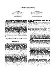
intentionally chosen to be close, making the processes harder to distinguish. Experiment 1. (Batch Setting) In this experiment we demonstrate that in the batch setting, the clustering errors corresponding to both the online and the offline algorithms converge to 0 as the sequencelengths grow. To this end, at every time-step t we take an N × n(t) sub-matrix X|n(t) of X composed of the rows of X terminated at length n(t), where n(t) = 5t. Then at each iteration we let each of the algorithms, (online and offline) cluster the rows of X|n(t) into five clusters, and calculate the clustering error-rate of each algorithm. As shown in Figure 2 (top) the error-rate of both algorithms decrease with sequence-length. Online Offline

0.5

mn = log n, in order to optimize running time. The choice of this parameter value is justified as follows: The expected waiting time before a word y = Y1..m is repeated within a sequence x = X1..n is inversely proportional to its probability of occurrence, P (y). For a sequence generated by an ergodic source with entropy rate h P (y) is asymptotically of order 2−mh . Therefore, counting the frequencies of words y = Y1..m in x for m > log n does not result in a consistent estimate of P (y). While the consistency of the distance estimates and thus the algorithm is not affected by this choice, it helps reduce the computational complexity (cf. Theorem 3.1). Apart from this choice of the parameters mn , no parameter tuning was used to achieve the empirical results (the values of the other parameters, such as the weights wj , were set to defaults described in Section 3).

2

We simulate α by a longdouble with a long mantissa.

0.4 0.3 0.2 0.1 0.0

200

300

400

0.2

0.3

0.4

0.5

Online Offline

0

For the purpose of our experiments, first we use five process distributions different processes DAS(αi ), i = 1..5, with α1 = 0.31..., α2 = 0.33..., α3 = 0.35..., α4 = 0.37..., α5 = 0.39. Next we generate an N × M data matrix X, each row of which is a sequence generated by one of the five DAS(αi ), i = 1..5 processes. Our task in both the online and the batch setting is to cluster the rows of X into k = 5 clusters. The selected αi are

100

Timestep

Mean of the Error Rate

Time-series generation. To generate a sequence x = X1..n we proceed as follows: Fix some parameter α ∈ (0, 1). Select r0 ∈ [0, 1]; then, for each i = 1..n obtain ri by shifting ri−1 by α to the right, and removing the integer part, i.e. ri := ri−1 + α − bri−1 + αc. The sequence x = (X1 , X2 , · · · ) is then obtained from ri by thresholding at 0.5, that is Xi := I{ri > 0.5}. We call this procedure DAS(α). If α is irrational then x forms a stationary ergodic time-series. 2

0

0.1

In this section we present empirical evaluations of our algorithms on synthetically generated data. To put the generality of our approach to a test, we have selected time-series distributions that, while being stationary ergodic, do not belong to any “simpler” general class of time-series, and are difficult to approximate by finitestate models. The considered processes are taken from [15], where they are used as an example of stationary ergodic processes that are not B-processes. Such timeseries cannot be modeled by a hidden Markov model with a finite or countably infinite set of states. Moreover, k-order Markov or hidden Markov approximations of this process do not converge to it in d¯ distance, a distance that is stronger than d, and whose empirical approximations are often used to study general (non-Markovian) processes (see, e.g. [10]).

Mean of the Error Rate

Synthetic Data

0.0

4.1

50

100

150

Timestep

Figure 2: Top: error-rate vs. sequence length in batch setting, Bottom: error-rate vs. # of observed samples in online setting. (error-rates averaged over 100 runs.) Experiment 2. (Online Setting) In this experiment we demonstrate that, unlike the online algorithm, the offline algorithm is consistently confused by the new sequences arriving at each time step in

Online Clustering of Processes

an online setting. To simulate an online setting, we proceed as follows: At every time-step t, a triangular window is used to reveal the first 1..ni (t), i = 1..t elements of the first t rows of the data-matrix X, with ni (t) := 5(t − i) + 1, i = 1..t. This gives a total of t sequences, each of length ni (t), for i = 1..t, where the ith sequence for i = 1..t corresponds to the ith row of X terminated at length ni (t). At every timestep t the online and offline algorithms are each used to in turn cluster the observed t sequences into five clusters. As shown in Figure 2 (bottom), in this setting the clustering error-rate of the offline algorithm remains consistently high, whereas that of the online algorithm converges to zero. 4.2

We compare our results against two other methods, namely those of [9] and [6], which (to the best of our knowledge) constitute the state-of-the-art performance on these datasets. Note that we have not implemented these reference methods, rather we have taken their numerical results directly from their corresponding articles. In order to have common grounds for each comparison we use the same sets of sequences,3 and the same means of evaluation as those used in [9, 6]. In [9] two MOCAP datasets4 are used, where the sequences in each dataset are labeled with either running or walking as annotated in the database. Performance is evaluated via the conditional entropy S of the true with respect to the prediction, i.e. Plabeling Mij Mij log P 0 M where M denotes S = − i,j P 0 0 M i0 j 0 ij 0 i ,j j the clustering confusion matrix. The motion sequences used in [9] are reportedly trimmed to equal duration. However, we use the original sequences as our method is not limited by variation in sequence lengths. Table 1 lists performance of Alg 1 as well as that reported for the method of [9]; Alg 1 performs consistently better. In [6] four MOCAP datasets5 are used, corresponding to four motions: run, walk, jump and forward jump. Table 2 lists performance in terms of accuracy. The datasets in Table 2 constitute two types of motions: 1. motions that can be considered ergodic (walk, run, marker position: the subject’s right foot. subjects #16 and #35. 5 subjects #7, #9, #13, #16 and #35. 4

1. 2.

Dataset Walk vs. Run (#35) Walk vs.Run (#16)

[9] 0.1015 0.3786

Alg 1 0 0.2109

Table 1: Comparison with [9]: Performance in terms of entropy; data-sets concern ergodic motion captures.

Real Data

As a real application we consider the problem of clustering motion capture sequences, where groups of sequences with similar dynamics are to be identified. Data is taken from the Motion Capture database (MOCAP) [1] which consists of time-series data representing human locomotion. The sequences are composed of marker positions on human body which are tracked spatially through time for various activities.

3

run/jog; displayed above the double line), and 2. nonergodic motions (single jumps; displayed below the double line). As shown in Table 2, Alg 1 achieves consistently better performance on the first group of datasets, while being competitive (better on one and worse on another) on the non-ergodic motions. The time taken to complete each task is in the order of few minutes on a standard laptop computer.

1. 2. 3. 4.

Dataset Run(#9) vs. Run/Jog(#35) Walk(#7) vs. Run/Jog(#35) Jump vs. Jump fwd.(#13) Jump vs. Jump fwd.(#13, 16)

[6] 100% 95% 87% 66%

Alg 1 100% 100% 100% 60%

Table 2: Comparison with [6]: Performance in terms of accuracy; Rows 1 & 2 concern ergodic, Rows 3 & 4 concern non-ergodic motion captures.

5

Outlook

The framework for clustering time-series considered in this work is fairly new, giving rise to many open problems and exciting directions for further research. While in this work we have assumed that the number of clusters k is known, in practice this may not be the case. Therefore, an interesting extension would be to consider the case of unknown number of clusters. As shown in [12] in general it is impossible to decide whether a pair of observed sequences are generated by the same or by two different stationary ergodic distributions. One mitigation is to make stronger assumptions on the data. Another approach often considered in the clustering literature is to construct a hierarchy of clustering for different k, in such a way that the true clustering is a pruning of this hierarchy. Acknowledgements This work is supported by the French Ministry of Higher Education and Research, Nord-Pas-de-Calais Regional Council and FEDER through CPER 20072013, ANR projects EXPLO-RA (ANR-08-COSI004) and Lampada (ANR-09-EMER-007), by an INRIA Ph.D. grant to Azadeh Khaleghi, by the European Community’s Seventh Framework Programme (FP7/2007-2013) under grant agreement 231495 (project CompLACS), and by Pascal-2.

Azadeh Khaleghi, Daniil Ryabko, J´ er´ emie Mary, and Philippe Preux

References [1] CMU graphics lab motion capture database. http://mocap.cs.cmu.edu/, 2009. [2] F.R. Bach and M.I. Jordan. Learning graphical models for stationary time series. IEEE Transactions on Signal Processing, 52(8):2189 – 2199, aug. 2004. [3] C. Biernacki, G. Celeux, and G. Govaert. Assessing a mixture model for clustering with the integrated completed likelihood. Pattern Analysis and Machine Intelligence, IEEE Transactions on, 22(7):719–725, 2000. [4] N. Cesa-Bianchi and G. Lugosi. Prediction, Learning, and Games. Cambridge University Press, 2006. [5] R. Gray. Probability, Random Processes, and Ergodic Properties. Springer Verlag, 1988. [6] T. Jebara, Y. Song, and K. Thadani. Spectral clustering and embedding with hidden Markov models. Machine Learning: ECML 2007, pages 164–175, 2007. [7] J. Kleinberg. An impossibility theorem for clustering. In 15th Conf. Neural Information Processing Systems (NIPS’02), pages 446–453, Montreal, Canada, 2002. MIT Press. [8] M. Kumar, N.R. Patel, and J. Woo. Clustering seasonality patterns in the presence of errors. In Proceedings of the eighth ACM SIGKDD international conference on Knowledge Discovery and Data mining, pages 557–563. ACM, 2002. [9] Lei Li and B. Aditya Prakash. Time series clustering: Complex is simpler! In Proceedings of the 28th International Conference on Machine Learning (ICML-11), pages 185–192, New York, NY, USA, June 2011. ACM.

[10] D.S. Ornstein and B. Weiss. How sampling reveals a process. Annals of Probability, 18(3):905–930, 1990. [11] D. Ryabko. Clustering processes. In Proc. the 27th International Conference on Machine Learning (ICML 2010), pages 919–926, Haifa, Israel, 2010. [12] D. Ryabko. Discrimination between B-processes is impossible. Journal of Theoretical Probability, 23(2):565–575, 2010. [13] D. Ryabko. Testing composite hypotheses about discrete ergodic processes. Test, 2012 (to appear). [14] D. Ryabko and B. Ryabko. Nonparametric statistical inference for ergodic processes. IEEE Transactions on Information Theory, 56(3):1430–1435, 2010. [15] P. Shields. The Ergodic Theory of Discrete Sample Paths. AMS Bookstore, 1996. [16] P. Smyth. Clustering sequences with hidden Markov models. In Advances in Neural Information Processing Systems, pages 648–654. MIT Press, 1997. [17] R. Zadeh and S. Ben-David. A uniqueness theorem for clustering. In A. Ng J. Bilmes, editor, Proceedings of the 25th Conference on Uncertainty in Artificial Intelligence (UAI’09), Montreal, Canada, 2009. [18] Shi Zhong and Joydeep Ghosh. A unified framework for model-based clustering. Journal of Machine Learning Research, 4:1001–1037, 2003.