Stability of Feature Selection Algorithms for ...

Stability of Feature Selection Algorithms for Classification in HighThroughput Genomics Datasets Panagiotis Moulos, Ioannis Kanaris, and Gianluca Bontempi, Senior Member, IEEE 

Abstract—A major goal of the application of Machine Learning techniques to high-throughput genomics data (e.g. DNA microarrays or RNA-Seq), is the identification of “gene signatures”. These signatures can be used to discriminate among healthy or disease states (e.g. normal vs cancerous tissue) or among different biological mechanisms, at the gene expression level. Thus, the literature is plenty of studies, where numerous feature selection techniques are applied, in an effort to reduce the noise and dimensionality of such datasets. However, little attention is given to the stability of these signatures, in cases where the original dataset is perturbed by adding, removing or simply resampling the original observations. In this article, we are assessing the stability of a set of well characterized public cancer microarray datasets, using five popular feature selection algorithms in the field of high-throughput genomics data analysis.

I. INTRODUCTION

D

the past fifteen years, the fields of molecular biology and genomics have witnessed incredible technological advances which continue to emerge. Established high-throughput techniques (e.g. DNA microarrays, [1]) or more recent ones (e.g. RNA-Seq, [2]) have allowed molecular biologists to quickly perform either large-scale descriptive studies (e.g. [3]) or to deeply investigate well-controlled biological systems and/or organism models. Although the experimental and clinical applications of high-throughput genomics are practically unlimited, a lot of effort has been put to the identification of gene expression “signatures” able to distinguish between healthy or pathological states or among disease states only, with particular focus in several cancer types. Such studies include breast cancer ([4, 5]), hematological cancers ([6, 7]), colon cancer ([8]) etc. To accomplish the goal of identifying comprehensive gene signatures, techniques from the Machine Learning field have been extensively used. For example, the aforementioned URING

Manuscript received July 25, 2013. The work of G.B. has been funded by ARC, French Community, Belgium P. M. is with the Institute of Molecular Biology and Genetics, BSRC „Alexander Fleming‟, 16672, Vari, Greece (corresponding author, phone: +30-210-9656310, e-mail: [email protected]). I. K. is with the Department of Information and Communication Systems Engineering, University of the Aegean, 83200, Karlovasi, Samos, Greece (e-mail: kanaris,[email protected]). G.B. is with the Machine Learning Group, Computer Science Department, Université Libre de Bruxelles and with the Interuniversity Institute of Bioinformatics in Brussels - (IB)2, 1050, Brussels, Belgium (email: [email protected]).

studies use a combination of feature selection and classification algorithms, where gene expression values comprise features/variables in a statistical model, and disease states represent the classes. In this work we examine the stability of five feature selection algorithms widely used in classification of microarray data, when the latter are subjected to perturbations. II. RELATED WORK The literature on feature selection stability is rather limited, let alone for biological applications. Previous studies introducing stability issues and proposing stability metrics include among others work by Kalousis et al., where stability is measured in terms of Pearson and Spearman correlation across ranked feature lists, as well as with an adaptation of the Tanimoto distance, [9]. Dunne et al. in [10] use the Hamming distance to assess the stability of selection by converting ranked lists to binary vectors. Regarding biomedical datasets, the issue is well defined by Lustgarten et al. in [11]. A complete study including feature selection performance, stability and classification accuracy using highthroughput data is presented by Haury et al. in [12]. However, the stability measurements are limited. III. MATERIALS AND METHODS A. Feature Selection Stability An important question arising during feature selection procedures is how sensitive a subset of ranked features is to perturbations. Specifically, let G = (g1, g2, …, gn) the total set of features/variables in a classification problem (e.g. the number of genes in a microarray) and let S1 = (g11, g12, …, g1N) a partial list of top N ranked features in ascending order obtained with feature selection algorithm A. If we apply a perturbation (e.g. bootstrapping the samples) and apply again A, we might obtain a different list S2 = (g21, g22, …, g2N). Some S1 members could correspond exactly to the members of S2 (presence and rank), some of them could have a different rank, or some that appear in S1 may not appear at all in S2. This issue is referred as the stability problem in feature selection ([13]) and is the main subject of the present work. Statistically, the sensitivity of feature selection can be formalized as a set of permutations of a full list Sn with n objects (n the number of features) where each of the n objects appears only once in each permutation of Sn

(permutation without replacement). Formally, a permutation π on a set Sn = (g1, g2, …, gn) of objects is a bijective function between Sn and Sn. In the frame of microarray data, the n genes involved in the problem are indexed with an integer between 1 and n and every ranked list is exactly a permutation π on the set {1,…, n}, where the image π(i) of the ith gene is its ranking inside the list π. Thus, π can be referred as a full ranking list of the objects of Gn. Furthermore, in the case of the top N ranked objects of Gn, we define as π* the partial ranking list of Gn which contains the first N elements of π. To assess the variability between such permutations we have to: i) summarize the difference between two full ranking lists π and σ and ii) summarize the difference between two partial ranking lists π* and σ*. In a theoretical context, the problem of comparing full ranking lists has been previously discussed in statistical literature (e.g in [14]) where metrics based on data ranking are used to compare full ranking lists (e.g. the Spearman’s Footrule). The problem of comparing partial ranking lists has also been studied ([14, 15]). The proposed solutions extend already existent metrics applied to full ranking lists by using the Hausdorff metric: (1) d H  A , B   m ax  m in d  a , b  a A

b B

B. Datasets For the purpose of this study, we used the following four publicly available and well studied cancer microarray datasets (two of them consisting of more than two classes): 1) The HBC dataset ([4]): this dataset consists of 3226 genes and 22 patients with hereditary breast cancer, sampled from three classes. The first two classes are labeled as “BRCA1” and “BRCA2” and they correspond to the mutation of the homonymous genes. The third class is named Sporadic, and corresponds to other genetic mutations. The dataset is randomly split to a test and a training set, holding out a random 25% of the samples (with classes equally distributed in the training and test sets). 2) The MLL dataset ([6]): this dataset consists of 12582 genes and 72 patients with three types of leukemia: 24 patients with ALL (Acute Lymphoblastic Leukemia), 28 patients with AML (Acute Myeloblastic Leukemia) and 20 patients with MLL (Mixed Lineage Leukemia). The dataset is split to training and test samples according to the original publication. 3) The ALL/AML Leukemia dataset (Golub, [7]): this dataset is historically one of the first datasets used for molecular classification of cancers based on microarray studies. The ALL and AML abbreviations are described in dataset (2). The set consists of 72 patients (47 ALL + 25 AML) and 7129 genes. The dataset is split to training and test samples according to [7]. 4) The B cell diffuse large cell lymphoma (B-DLCL) dataset ([16]): this dataset consists of 47 patients, 4026

genes and two classes: 24 patients with germinal center B cell-like DLCL and 23 patients with activated B celllike DLCL. From the 24 samples of the first class and the 23 of the second, 6 samples of each are held as testing samples and the other used for training. C. Feature Selection Algorithms We applied five widely used feature selection methods, which function independently of the classifier (filters): i) the Student‟s t-test between samples of different classes, ii) the Pearson and iii) the Spearman‟s correlation, between the gene expression values and the class assignment vector, iv) the Information Gain filter and v) the Gini index. The number of top scored features that we stored after each perturbation was N=100. While selecting N was trivial for the 2-class datasets, for the multiclass datasets we performed the feature selection for all possible C one-vs-rest comparisons (where C is the number of classes). Then, we built the final feature sets by selecting N/C top features from each comparison, where . is the ceiling function. D. Stability of Selection Definition: The stability of feature selection for a given dataset and selection algorithm is the stability of appearance of the selected high-score features upon applying a perturbation scheme on the original dataset. We measure the stability of selection with an alternative of the Hamming distance as proposed in [10]. Given two binary vectors li, lj, the Hamming distance between them is H  li , l j  

n



(1)

l ik  l jk

k 1

Given a list of features S, where each feature is assigned a number from 1…n, n the total number of features, the list can be represented by a binary vector l of length n (feature mask), where 0s represent the absence of a specific feature and 1s represent its presence. Thus, the similarity between two feature masks can be measured by the Hamming Distance as defined above. Furthermore, in order to measure the similarity between all pairs of partial ranking lists produced after m MC iterations, we define the total Hamming Distance between m feature masks as m 1 m m 1 m n (2) H  H l ,l  l l



 

i

j

 

i 1 j  i  1

ik

jk

i 1 j  i  1 k 1

We normalize (2) by dividing by Ni + Nj, where Ni and Nj are the top ranked features selected in MC iterations i and j respectively. The sum Ni + Nj represents the maximum possible different features (and consequently the maximum Hamming distance) between two feature masks and Ni + Nj  2N. Finally, we define the mean normalized Hamming distance for all the m(m-1)/2 pairwise feature mask distances of m MC iterations as m 1 m n (3) 2 1 H n o rm  1 

m  m  1



i 1 j  i  1

Ni  N



l ik  l jk

j k 1

Hnorm lies between 0 and 1. A value close to 0 represents

low stability while a value close to 1 represents high stability. To illustrate an example, let S1 = (1,2,3), S2 = (2,4,5), m = 2, n = 5 and N = 3. S1 and S2 lead to the feature masks l1 = (1,1,1,0,0) and l2 = (0,1,0,1,1), thus Hnorm = 1 – (1/6)*(1 + 0 + 1 + 1 + 1) = 0.3333. E. Stability of Ranking Definition: The stability of feature ranking for a given dataset and selection algorithm is the stability of both the appearance and the ranking order of the selected high-score features upon applying a perturbation scheme on the original dataset. In order to measure the stability of feature ranking we apply an alternative of the Spearman’s Footrule ([14]), a metric based on the Hausdorff distance, which can be used for measuring the stability of ranking for partial ranked lists. Before its definition, we first explain certain required notation elements: let Si, Sj two partial ranking lists (as in III.A), π and σ the full ranking lists of Si, Sj respectively, m the number of perturbation iterations, n the total number of features and N the number of top ranked features we use to build the high score feature lists. Let also A, B, D, E the following partitions of the n features: A   u  1, ..., n :   u   N ,   u   N  B   u  1, ..., n :   u   N ,   u   N 

E   u  1, ..., n :   u   N ,   u   N 

This means that A consists of all features ranked in the top N by both π and σ, B consists of all features ranked in the top N by π but not by σ, and so on. Let also h = |B| = |D|, the number of elements in the sets B and D. We can now define the Spearman’s Footrule for partial ranking lists: (5) SF  S , S     u    u   h  2n  1  h     u     u  i

j

u A

u B

u D

The SFp can be normalized by its maximum value which can be calculated if we consider the most distant partial ranking lists between n objects, which are Slow = (1,…,N) and Shigh = (n,…,n – N + 1). Thus, SFp,max = SFp(Slow, Shigh). We also define the mean value of SFp for all the m(m-1)/2 pairwise distances of m perturbations as: SF

p , norm

1

2 m  m  1  S F p , m ax



    u    u   h  2n  1  h    u A

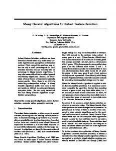
IV. RESULTS AND DISCUSSION A. Visualization of Feature Selection Instability Fig. 1 depicts the feature selection stability by plotting the feature index (1…N) against the frequency that a specific feature appears during the feature selection process after applying m=100 perturbations.

(4)

D   u  1, ..., n :   u   N ,   u   N 

p

Carlo (MC) simulations performed on each dataset. In each MC iteration, the samples of the original dataset are bootstrapped, creating a new instance of the feature selection problem with slightly altered initial conditions (different sets of samples for each class).

   u     u   uB uD 

(6)

A value of SFp,norm closer to 0 means low stability while a value closer to 1 means high stability. To illustrate an example, let π = (1,2,3,5,4), σ = (2,4,5,1,3), S1 = (1,2,3), S2 = (2,4,5), m = 2, n = 5, N = 3. Then A = {1}, B = {2,3}, D = {4,5}, E = , |A| = 1, |B| = |D| = 2, |E| = 0 and thus SFp,norm = 1 – (1/12)*2*(2*5 + 1 – 2) + |1 – 2| – (2 + 3) – (1 + 3) = 0.1667 F. Perturbation scheme As perturbation scheme, we chose a set of 100 Monte

Fig 1: Frequencies of selected features (genes) for the HBC (three classes) and the Golub (two classes) datasets, using the Pearson correlation-based selection method and the Information Gain filter.

From Fig. 1, it is evident that certain features are selected more frequently than others during the selection-perturbation loop and the frequency depends i) on the method used and ii) on the complexity of the dataset. Thus, it appears than in both cases depicted in Fig. 1, Pearson correlation-based selection performs better than Information Gain in terms of stability. However, stability is increased for both methods in the case of the Golub dataset (2-class problem) as compared to the HBC dataset (three classes). B. Stability Measurements Fig. 2 presents bar charts depicting the stability of selection for each dataset and for each feature selection method applied in this study. The first observation after the completion of the simulation is that the overall stability of selection is not greater than 45%. This indicates that the filter-based feature selection procedure is a process very sensitive to perturbations, at least in the context of biomedical high-throughput datasets. Thus, it should be taken into account when the aim of the study is the derivation of a gene signature characterizing disease. In addition, the stability of selection is generally higher for feature sets derived from 2-class datasets than from multiclass datasets, something to be expected due to the higher complexity of the latter. This appears to be partially remedied by the number of available samples, as the stability

is higher for the MLL dataset than for the HBC dataset. The latter shows the lowest stability during the perturbationfeature selection loop and we attribute this to the small number of samples related to the number of classes and the number of features in the dataset.

dimensionality of classification problems in high-throughput genomics. We have demonstrated that feature selection is a sensitive process and its stability must be taken into account in studies aiming at deriving gene signatures that distinguish between pathological states. In the future, we will extend our study by assessing the stability of several publicly available datasets using additional metrics of feature selection stability, over additional feature selection algorithms. We will also measure the effect of dataset perturbation and subsequent feature selection in prediction accuracy, using well established classifiers. REFERENCES [1] [2]

Fig. 2: Stability of selection for each feature selection method and each datasets used in this study.

Finally, the overall best performance can be attributed to the correlation based methods, followed by the Information Gain and Gini index. The t-test demonstrates the poorest performance. Similarly to the case of stability of selection, Fig. 3 presents bar charts depicting the stability of ranking for the same settings.

[3]

[4]

[5]

[6]

[7]

[8]

Fig. 3: Stability of ranking for each feature selection method and each datasets used in this study.

From Fig. 3 it is evident that the stability of ranking is proportional to the stability of selection, with the t-test being the less robust selection method and the HBC dataset demonstrating the poorest stability. Thus, the extent of variability in terms of different features selected after dataset perturbation appears similar to the extent of variability in terms of feature priority in the different signatures. Consequently, the stability of ranking can be used as a combined measurement of gene signature stability, as it appears able to capture both the stability selection and ranking attributes of gene signatures. CONCLUSIONS AND FUTURE WORK In this article, we have studied the stability of several feature selection algorithms used to reduce the

[9] [10]

[11] [12] [13] [14] [15] [16]

Tarca AL, Romero R, Draghici S: Analysis of microarray experiments of gene expression profiling. American journal of obstetrics and gynecology 2006, 195(2):373-388. Wang Z, Gerstein M, Snyder M: RNA-Seq: a revolutionary tool for transcriptomics. Nat Rev Genet 2009, 10(1):57-63. Birney E, Stamatoyannopoulos JA, Dutta A, Guigo R, Gingeras TR, Margulies EH, Weng Z, Snyder M, Dermitzakis ET, Thurman RE et al: Identification and analysis of functional elements in 1% of the human genome by the ENCODE pilot project. Nature 2007, 447(7146):799-816. Hedenfalk I, Duggan D, Chen Y, Radmacher M, Bittner M, Simon R, Meltzer P, Gusterson B, Esteller M, Kallioniemi OP et al: Geneexpression profiles in hereditary breast cancer. N Engl J Med 2001, 344(8):539-548. Loi S, Haibe-Kains B, Desmedt C, Wirapati P, Lallemand F, Tutt AM, Gillet C, Ellis P, Ryder K, Reid JF et al: Predicting prognosis using molecular profiling in estrogen receptor-positive breast cancer treated with tamoxifen. BMC Genomics 2008, 9:239. Armstrong SA, Staunton JE, Silverman LB, Pieters R, den Boer ML, Minden MD, Sallan SE, Lander ES, Golub TR, Korsmeyer SJ: MLL translocations specify a distinct gene expression profile that distinguishes a unique leukemia. Nat Genet 2002, 30(1):41-47. Golub TR, Slonim DK, Tamayo P, Huard C, Gaasenbeek M, Mesirov JP, Coller H, Loh ML, Downing JR, Caligiuri MA et al: Molecular classification of cancer: class discovery and class prediction by gene expression monitoring. Science 1999, 286(5439):531-537. Bertucci F, Salas S, Eysteries S, Nasser V, Finetti P, Ginestier C, Charafe-Jauffret E, Loriod B, Bachelart L, Montfort J et al: Gene expression profiling of colon cancer by DNA microarrays and correlation with histoclinical parameters. Oncogene 2004, 23(7):1377-1391. Kalousis A, Prados J, Hilario M: Stability of feature selection algorithms: a study on high-dimensional spaces. Knowledge and Information Systems 2007, 12(1):95-116. Dunne K, Cunningham P, Azuaje F: Solutions to Instability Problems with Sequential Wrapper-Based Approaches To Feature Selection. Technical Report TCD-CS-2002-28, Department of Computer Science, Trinity College, Dublin, Ireland 2002. Lustgarten JL, Gopalakrishnan V, Visweswaran S: Measuring stability of feature selection in biomedical datasets. AMIA Annu Symp Proc 2009, 2009:406-410. Haury AC, Gestraud P, Vert JP: The influence of feature selection methods on accuracy, stability and interpretability of molecular signatures. PLoS One 2011, 6(12):e28210. Guyon I, Elisseeff A: An Introduction to Variable and Feature Selection. Journal of Machine Learning Research 2003, 3:1157-1182. Critchlow DE: Metric Methods for Analyzing Partially Ranked Data, vol. 34: Springer-Verlag; 1985. Fagin R, Kumar R, Sivakumar D: Comparing top k Lists. In: ACMSIAM symposium on Discrete Algorithms: 2003; 2003: 28-36. Alizadeh AA, Eisen MB, Davis RE, Ma C, Lossos IS, Rosenwald A, Boldrick JC, Sabet H, Tran T, Yu X et al: Distinct types of diffuse large B-cell lymphoma identified by gene expression profiling. Nature 2000, 403(6769):503-511.