Investigation of genetic algorithms contribution to feature selection for

International Journal of Remote Sensing Vol. 30, No. 3, 10 February 2009, 611–625

Investigation of genetic algorithms contribution to feature selection for oil spill detection K. TOPOUZELIS*{{, D. STATHAKIS{ and V. KARATHANASSI{ {Joint Research Centre (JRC) of the European Commission, Institute for the Protection and Security of the Citizen, Ispra, 21020 (VA), Italy {Laboratory of Remote Sensing, School of Rural and Surveying Engineering, National Technical University of Athens, Heroon Polytechniou 9, GR-15780, Greece (Received 8 May 2007; in final form 19 November 2007 ) Oil spill detection methodologies traditionally use arbitrary selected quantitative and qualitative statistical features (e.g. area, perimeter, complexity) for classifying dark objects on SAR images to oil spills or look-alike phenomena. In our previous work genetic algorithms in synergy with neural networks were used to suggest the best feature combination maximizing the discrimination of oil spills and look-alike phenomena. In the present work, a detailed examination of robustness of the proposed combination of features is given. The method is unique, as it searches though a large number of combinations derived from the initial 25 features. The results show that a combination of 10 features yields the most accurate results. Based on a dataset consisting of 69 oil spills and 90 lookalikes, classification accuracies of 85.3% for oil spills and in 84.4% for look-alikes are achieved.

1.

Introduction

Synthetic Aperture Radar (SAR) images are extensively used for the detection of oil spills in the marine environment, as they are independent from sun light and they are not affected by cloudiness. Radar backscatter values from oil spills are very similar to backscatter values from very calm sea areas and other ocean phenomena named ‘look-alikes’ (e.g. currents, eddies, upwelling or downwelling zones, fronts and rain cells). Several studies aiming at oil spill detection have been conducted (Solberg and Theophilopoulos 1997, Espedal and Wahl 1999, Solberg et al. 1999, Del Frate et al. 2000, Espedal and Johannessen 2000, Fiscella et al. 2000, Pavlakis et al. 2001, Topouzelis et al. 2003, Keramitsoglou et al. 2005, Karathanassi et al. 2006). A detailed introduction to oil spill detection by satellite remote sensing is given in Brekke and Solberg (2005). The basic methodology of oil spill detection can be summarized in four steps (Pavlakis et al. 2001, Solberg et al. 1999, Brekke and Solberg 2005). First, all dark signatures present in the image are isolated. Second, features for each dark signature are extracted. Third these features are tested against predefined values. Finally, probabilities for each candidate signature are computed to determine whether it is an oil spill or a look-alike phenomenon. The absence of systematic research on features extracted and their contribution to the classification results forces researchers to select features arbitrarily as input to *Corresponding author. Email: [email protected] International Journal of Remote Sensing ISSN 0143-1161 print/ISSN 1366-5901 online # 2009 Taylor & Francis http://www.tandf.co.uk/journals DOI: 10.1080/01431160802339456

612

K. Topouzelis et al.

their systems. A previous work (Stathakis et al. 2006) was focused on this issue, trying to bridge this chasm and to discover the most useful features in oil spill detection. The lack of systematic research can be attributed to the fact that the existing methodologies for searching into a large number of different compilations have not been fully exploited. Genetic algorithms have been successful in discovering an optimal or near-optimal solution amongst a huge number of possible solutions (Goldberg 1989). Moreover, a combination of genetic algorithms and neural networks can prove to be very powerful in classification problems. The methodology of feature selection for oil spill detection is given in Stathakis et al. (2006). The 25 most commonly used features in the scientific community were grouped and their contribution to the final classification was examined. The methodology explores the opportunity of having two unknown parameters in the genetic internal structure, i.e. the number of input features and the number of hidden neurons. The novelty of this approach is the simultaneous evolution of both features and neural network topology. Previously genetic algorithms have been used either to evolve neural network topology (Stathakis and Kanellopoulos 2006) or to select features (Kavzoglou and Mather 2002) but not both at the same time. Thus, a novel synergy of genetic algorithms and neural networks is deployed in order to determine a near-optimal neural network for the classification of oil spills and lookalikes. The present paper evaluates the robustness of the proposed feature combination. In order to further justify the proposed feature combination robustness a comparison with the results of several commonly used reparability indices, including Euclidian, Fisher and Mahalanobis, was performed. 2.

Features related to oil spill detection

Features can be generally grouped in three major categories (Solberg and Theophilopoulos 1997, Solberg et al. 1999, Del Frate et al. 2000, Karathanassi et al. 2006, Brekke and Solberg 2005): those referring to the geometric characteristics of oil spills (e.g. area, perimeter, complexity); those capturing the physical behaviour of oil spills (e.g. mean or max backscatter value, standard deviation of the dark formation or a bigger surround area); and features referring to the oil spill context in the image (e.g. number of other dark formations in the image, presence of ships). Fiscella et al. (2000) used 14 features for oil spill classification; five of them for the geometry and nine for the backscattering behaviour. Solberg and Theophilopoulos (1997) used 15 features; four of them for the geometry, eight for the physical behaviour and three for the context of the oil spills. Solberg et al. (1999) used 11 features, many of them different from their previous studies and in general different from the 11 features used by Del Frate et al. (2000). A different approach was given by Espedal and Wahl (1999), in which wind vector data were used and compared with the spreading and length of the dark formations detected. A more general description of the calculated features was given by Espedal and Johannessen (2000), where texture features were introduced for the first time. Moreover, Keramitzoglou et al. (2005) referred to 14 features without presenting them and Karathanassi et al. (2006) used 13 features covering physical, geometrical and textural behaviour. Several studies have tried to unify all the features used with similar characteristics (Brekke and Solberg 2005, Montali et al. 2006). Table 1 presents a grouping of the 25 most commonly used features applied in the majority of research studies as well as in the present study. The first six features (1–6) refer to the geometrical characteristics, the next 16 features (7–22) refer to the physical characteristics and

No Area Perimeter Perimeter to area ratio Complexity Shape factor I

Features

SP2

A P P/A C SP1

Code

x Spreading

x x

Frate et al., 2000 x

Solberg et al, 1999

Table 1. Features used for oil spill detection.

1 2 3 4 5 Shape factor II

7 8 9 10 Background standard deviation Background power to mean ratio Ratio of the power to mean ratios Mean contrast Max contrast

Object mean value Object standard deviation Object power to mean ratio Background mean value

ConRaMe ConRaSd ConLa GMe GSd

BSd Bpm Opm/Bpm ConMe ConMax

OMe OSd Opm BMe

x x

x x

First invariant planar moment x

Homogeneity

x x

x x x

Fiscella et al., 2000

Large areas

Karathanassi et al., 2006

Asymmetry

Shape Index Length to width ratio Form factor

x

x

x x x x x x x

x x x

x x x x

Feature selection for oil spill detection

x

x Slick width

6

11 12 13 14 15 Mean contrast ratio Standard deviation contrast ratio Local area contrast ratio Mean border gradient Standard deviation border gradient

GMax NDm TSp TSh THm

x

16 17 18 19 20 Max border gradient Mean Difference to Neighbours Spectral texture Shape texture Mean Haralick texture

x

21 22 23 24 25

613

614


the last three (23–25) to the texture characteristics of the dark formations. In detail the features shown in table 1 are: 1. Area (A): area of the object. 2. Perimeter (P): length of the border of the object. 3. Perimeter to area ratio (P/A): the ratio between the perimeter (P) and the area (A) of the object. 4. Object complexity (C): describes how simple (or complex) the geometrical objects are. It can be calculated in different ways (see table 1). 5. Shape factor I (SP1): describes how long and thin objects are. It has been referred to as ‘spreading’, ‘slick width’ and as ‘length to width ratio’ (see table 1). 6. Shape factor II (SP2): describes the general shape of the object. It has also been referred to as ‘first invariant planar moment’, ‘form factor’ and ‘asymmetry’ (see table 1). First invariant planar moment (Hu 1962, Solberg et al. 2007) is defined as W15g20 + g02, where gpq is the normalized central moment, gpq5mpq/m00, and mpq is the non-normalized central moment. Form factor computes the dispersion of dark area pixels from the longitudinal axis. Asymmetry computes the ratio of the lengths of minor and major axes of an ellipse describing the object shape. 7. Object mean value (OMe): mean of the intensity values of the pixels belonging to the oil spill candidate. It describes how dark the oil spill candidate is. 8. Object standard deviation (OSd): standard deviation of the intensity values of the pixels belonging to the oil spill candidate. 9. Object power to mean ratio (Opm): the ratio between the standard deviation (OSd) and the mean (OMe) values of the object. 10. Background mean value (BMe): mean of the intensity values of the pixels belonging to the region of interest, selected by the user surrounding the object. 11. Background standard deviation (NSd): standard deviation of the intensity values of the pixels belonging to the region of interest, selected by the user surrounding the object. 12. Background power to mean ratio (Bpm): the ratio between the standard deviation (NSd) and the mean (BMe) values of background. 13. Ratio of the power to mean ratios (Opm/Bpm): the ratio between the object power to mean ratio (Opm) and the background power to mean ratio (Bpm). This describes the difference in distribution of the backscatter values between the oil spill candidate and the background area. 14. Mean contrast (ConMe): the difference between the background mean value (BMe) and the object mean value (OMe). 15. Max contrast (ConMax): the difference between the background mean value (BMe) and the lowest value inside the object. 16. Mean contrast ratio (ConRaMe): the ratio between the object mean value (OMe) and the background mean value (BMe). 17. Standard deviation contrast ratio (ConRaSd): the ratio between the object standard deviation (OSd) and the background standard deviation (BSd). 18. Local area contrast ratio (ConLa): the radio between the mean backscatter value of the object (OMe) and the mean backscatter value of a window centred at the region. This describes the difference between the mean backscatter value of the candidate oil spill and the mean backscatter value of a local area.


615

19. Mean border gradient (GMe): the mean of the magnitude of gradient values of the region border area. The Sobel operator is used to compute the gradients. It describes how dark the border gradient of the candidate oil spill is. 20. Standard deviation border gradient (GSd): this describes the backscatter values spreading of the border gradient of the candidate oil spill. 21. Max border gradient (GMax): maximum value of the border gradient values. This gives the maximum backscatter value of the border gradient of the candidate oil spill. 22. Mean difference to neighbours (NDm): for each neighbouring object, the mean difference is computed and multiplied with the shared border length between the objects. This describes the differences of the mean value of the candidate oil spill and the surrounding areas weighted by the common border length they have. 23. Spectral texture (TSp): the spectral texture based on sub-objects. It analyses the texture of the spectral information provided by the original image layer and is calculated as the standard deviation of the different mean values of the sub-objects. It describes the mean backscatter values spreading from small areas (i.e. sub-objects) which are forming the candidate oil spill. 24. Shape texture (TSh): the shape texture based on sub-objects. It analyses the form of sub-objects and is calculated as the standard deviation of the asymmetries of the sub-objects. 25. Mean Haralick texture (THm): the mean Haralick texture (Haralick 1979) based on sub-objects. It is calculated as the average of the grey level cooccurrence matrices of the sub-objects. The present study, due to nature of the data used, does not include features referring to the context of the oil spills in the image, such as those presented in Solberg et al. (1999), i.e. distance to a point source, number of detected spots in the scene and number of neighbouring spots; or those presented in Karathanassi et al. (2006), i.e. distance from large areas, land and fractal objects. Context features are not included because the computation of the rest features requires isolation of the dark areas from the original images first. As a consequence no contextual information could be derived. 3.

Dataset

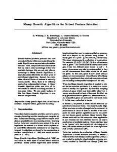
Most studies use low resolution SAR data (quick-looks), with nominal spatial resolution of 100 m6100 m, to detect oil spills (Solberg and Theophilopoulos 1997, Espedal and Wahl 1999, Solberg et al. 1999, Del Frate et al. 2000, Espedal and Johannessen 2000, Fiscella et al. 2000, Pavlakis et al. 2001, Keramitsoglou et al. 2005). Low resolution data are sufficient for large scale monitoring. Small and fresh spills however cannot be as efficiently detected (Karathanassi et al. 2006). To evaluate the proposed methodology this study used a dataset of 24 high-resolution SAR images (PRI SAR product with 100 km swath width), with spatial resolution of 25 m625 m. The dataset contains several sea states. All images contain several dark objects and have previously been used in different studies (Pavlakis et al. 2001, Karathanassi et al. 2006). An example of an oil spill and a look-alike is shown in figure 1. To speed up the process, the method was applied on windows rather than complete scenes of the European Remote Sensing satellite 2 (ERS-2). From the 24 SAR images, 159 image windows were extracted, containing 90 look-alikes and 69 oil spills. Look-alikes can be low wind areas, organic film, wind front areas, areas

616


Figure 1. Examples of (a) verified oil spill, (b) verified look-alike taken on 6 September 2005 close to Ancona, Italy (orbit: 54270 Frame: 2727). Verification was done by Italian coastguards with aircraft inspection of the locations.

sheltered by land, rain cells, current shear zones, grease ice, internal waves and upwelling (or downwelling) zones (Alpers et al. 1991, Hovland et al. 1994). In the present work all these types were used, with the exception of grease ice. Table 2 contains the main statistical parameters of the features used for the given dataset. We randomly split the available dataset into two equally sized parts. One was used for training and the other for testing in the neural network classification. Both sets contain almost equal numbers of look-alikes and oil-spills. For each dark object selected in the above-mentioned image windows, a set of 25 features was extracted. Note that the operation was done on objects rather than pixels. Dark formations are detected using an object-oriented methodology described in detail by Topouzelis et al. (2003) and by Karathanassi et al. (2006). 4.

Methodology – computational intelligence for oil spill detection

In this paper we use computational intelligence (Stathakis and Vasilakos 2006), which refers here to the synergy of neural networks and genetic algorithms. The

617


Table 2. Main statistical parameters describing the features extracted from the dataset (St. Dev. is standard deviation). OIL SPILLS Feature A SP2 BMe P Bpm

Min

Max

Mean

LOOKALIKES St.Dev

382.00 346550.00 30471.09 55930.64 0.15 1.00 0.86 0.19 78.94 172.21 115.94 18.56 138.00 25290.00 2812.06 3823.01 0.25 0.54 0.39 0.08

Min

Max

Mean

St.Dev

401.00 907090.00 47242.99 116988.16 0.05 1.00 0.72 0.26 78.12 168.74 113.97 17.52 192.00 32326.00 4233.16 5038.28 0.25 0.54 0.42 0.07

BSd ConLa ConMax ConMe ConRaMe

26.83 0.15 77.60 23.36 0.15

59.87 0.76 157.21 121.29 0.80

44.28 0.39 113.08 72.36 0.38

8.52 0.13 18.02 20.67 0.14

26.57 0.18 71.54 23.84 0.17

57.90 0.75 163.53 116.05 0.75

46.80 0.45 112.83 67.58 0.41

7.81 0.14 17.56 21.27 0.14

ConRaSd GMax GMe GSd SP1

0.39 141.00 54.19 21.10 1.05

0.91 255.00 149.36 51.60 22.99

0.63 226.62 79.85 37.90 5.72

0.10 34.11 14.38 7.87 4.80

0.47 140.00 42.83 18.79 1.02

0.87 255.00 110.51 51.98 22.29

0.65 234.92 79.11 38.24 4.06

0.10 28.72 11.66 7.50 4.51

NDm OMe Opm Opm/Bpm OSd

10.56 17.37 0.30 1.04 12.84

65.98 130.33 1.31 3.61 43.35

35.86 43.57 0.72 1.84 27.92

12.44 18.07 0.29 0.62 7.19

6.29 17.44 0.27 1.06 15.90

63.74 91.45 1.60 3.08 47.09

31.84 46.40 0.72 1.73 30.32

13.36 15.39 0.26 0.54 6.51

P/A C THm TSh TSp

0.02 1.51 18.36 0.17 14.79

0.75 11.77 130.41 0.24 51.47

0.21 4.33 44.52 0.22 33.84

0.14 2.40 17.69 0.01 8.44

0.03 1.58 19.22 0.21 18.14

0.95 16.28 91.58 0.29 58.06

0.25 6.02 47.42 0.23 36.37

0.19 2.56 14.85 0.01 7.58

genetic algorithm is used in order to identify the input feature combination that gives the highest classification accuracy. A detailed introduction to computational intelligence for oil spill detection can be found in Stathakis et al. (2006). Although there are several examples in the literature of the use of genetic algorithms in optimization problems, few are applications in remote sensing. The chromosome string representation was used to code the information for use with the neural network. In each individual string there is information both for the combination of features that currently participate in the solution and for the number of nodes in the hidden layer. We chose to limit the search for neural network topologies to skeletons that only contain one hidden layer. We base this choice on the Kolmogorov theorem (Atkinson and Tatnall 1997), which states that a neural network with only one hidden layer is enough to model any function regardless of complexity. A second hidden layer could be easily implemented in the same system if required. The first part of the string contains one bit per input dimension. The value of 1 denotes the presence of this feature in the solution, and the value of 0 its absence. We used 25 input dimensions and we needed an equal number of bits to code the features into each individual string. The second part of the string contains seven bits in the string to code the number of nodes in the hidden layer, which are enough to represent the numbers 0–127. We added the value of 1 to this 7-bit number so that the result is 1–128, avoiding the null topology. Topology selection is a well-known

618


problem in neural networks. No exact solution exists currently. Several heuristic rules have been introduced however to amend this problem. In the present study, the choice of how many hidden nodes we should search and thus how many bits are needed in the chromosome string was based on the Kanellopoulos–Wilkinson rule (Kanellopoulos and Wilkinson 1997). This rule proposes a structure for the neural network used, where the number of hidden nodes should be at last equal to double the number of inputs or outputs, whichever is larger, and perhaps four times as many to be safe. The application of this rule to our data, which have as a maximum 25 inputs (features) and always two outputs (oil spill or look-alike), yields the 25 : 100 : 2 topology as the maximum topology (high bound) that is to be explored. To evaluate the suitability of each discovered solution we used the fitness function proposed by Siedlecki and Sklansky (1989). We used a genetic algorithm with population set to 20. The population contains individual solutions that are mixed with the generation to follow in order to produce superior solutions. Each solution is a chromosome. A two-point crossover with value 0.9 was used. Crossover is the mixing of two solutions (chromosomes) in order to create two new solutions. Twopoint crossover means that each of the two parent chromosomes is split into two points and the resulting parts are subsequently interchanged. In mutation, one bit in the chromosome is randomly flipped at a very low rate. It is used to ensure that the algorithm is not limited by the genetic material provided in the initial population of solutions. Here Gaussian mutation was used. Each individual solution (chromosome) was selected for reproduction according to each fitness, so that better solutions produce more children and hence the probability of discovering a superior solution in the following generations is higher. Here tournament selection was used, which means that the population is split into groups and the best individual in each group are selected for reproduction. The neural network used is a standard fully connected feedforward multi-layer perceptron trained by the backpropagation algorithm (Rumelhart and McClelland 1986). In fact, for faster training we used the Levenberg-Marquardt version of backpropagation (Hagan and Menhaj 1994). Log sigmoid transfer function was used and we set learning rate to 0.03 and momentum to 0.9. The maximum number of epochs to complete was 110. Each time the genetic algorithm produces a new solution as a chromosome string, a neural network is actually built from this string, having a number of inputs equal to the number of features present in the string and a number of hidden nodes equal to the number in the string plus one (to avoid null topologies). After the neural network was created, it was trained with the backpropagation variant using the training set. The testing set was then classified using the set of weights discovered during training. The accuracy matrix (Congalton and Green 1998) on the testing set data was created and the overall classification accuracy was calculated. This number was then passed to the fitness function (Siedlecki and Sklansky 1989) and the value for each chromosome string was calculated and passed back to the genetic algorithm to continue searching for solutions. 5.

Analysis of the genetic algorithm results

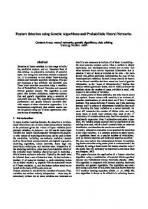
In general the results show that the method presented here is very efficient in determining an optimal subset of features as well as an optimal hidden layer topology. The evolution of number of features is shown in figure 2 and the evolution of topology is shown in figure 3. As we can see from the two figures the number of


Figure 2.

619

Number of features used through generations.

the used features and the number of the hidden nodes are stabilized after 10 generations for the former and after 30 generations for the latter. The best set of features discovered by the proposed method contains nine: [SP2, BSd, ConLa, Opm, Opm/Bpm, OSd, P/A, C, THm]. This solution yields 84.8% overall testing accuracy. It is discovered after 32 generations and is achieved with 51 nodes in the hidden layer. From the testing dataset of 34 oil spills only five were misclassified as lookalikes, resulting in 85.3% oil spill producer’s accuracy. From the 45 testing cases of look-alikes, seven were misclassified as oil spills, representing 84.4% producer’s

Figure 3.

Number of hidden nodes through generations.

620


accuracy level. Our training data were all classified correctly in the case of lookalikes (45 look-alikes) while only one misclassified in case of oil spills (35 cases). It is worth mentioning here that because of the relatively small training set size, effort has been made to include as many different cases of oil spills and look-alikes as possible. Moreover, the dataset is randomly split into two parts: one for training and one for validation. This means in practice that the validation part contains as many randomly chosen different oil spills and look-alikes as possible, which are kept independent of training. This procedure aims to strengthen the reliability of the results. By looking at the 20 best performing solutions we see that all except the best one have 10 features. The features common in all solutions are [SP2, BSd, ConLa, GMe, Opm, Opm/Bpm, OSd, P/A, C] whereas the additional feature is THm in all except one case, where TSp is present instead. From the selected features three referred to geometrical characteristics (P/A, C, SP2), six to physical characteristics (OSb, Opm, BSd, Opm/Bpm, ConLa, GMe) and only one to texture characteristics (THm). In our case the genetic algorithm evaluated 2020 solutions (chromosomes) in total. All features were used more than once. Table 3 presents the percentage of the times each feature was used. Three features were used less than 20 times: ConRaMe, GMax and TSh. The two first were used 12 times (i.e. 0.6%) and the latter 18 times (i.e. 0.9%). Then, 11 features (A, BMe, P, Bpm, ConMax, ConMe, GSd, SP1, NDm, OMe, TSp) were used between 28 and 93 times (i.e. 1.4–4.6%) and the remaining 11

Table 3. Number of times that the features were used, expressed as a percentage. No

Features

Times used (%)

Times used

1 2 3 4 5

A SP2 BMe P Bpm

0.1 100 0.5 0.5 0

1 1500 7 7 0

6 7 8 9 10

BSd ConLa ConMax ConMe ConRaMe

99.6 100 0.3 0.5 0

1494 1500 5 7 0

11 12 13 14 15

ConRaSd GMax GMe GSd SP1

0.3 0 99.5 0.7 0.7

5 0 1492 10 11

16 17 18 19 20

NDm OMe Opm Opm/Bpm OSd

1.3 1.9 98.6 99.3 99.7

20 28 1479 1489 1496

21 22 23 24 25

P/A C THm TSh TSp

100 100 96.9 0 3.7

1500 1500 1454 0 56


621

(SP2, BSd, ConLa, ConRaSd, GMe, Opm, Opm/Bpm, OSd, P/A, C, THm) were used more than 1990 times (i.e. 96%). If we exclude the worst 520 cases that present large errors and anomalies, and focus on the first 1500 best performing solutions (chromosomes), we will notice that four features are not used at all (Bpm, ConRaMe, GMax, Tsh), while feature A is used only once. From the 1500 best performing solutions 1386 contain the same combination of 10 features. The remaining 114 solutions can be divided in chromosomes containing 10 features and chromosomes not containing 10 features. Apparently 42 out of the 47 in total chromosomes containing 10 features, Tsp feature is used instead of THm. For the remaining five chromosomes, four used OMe instead of Opm and one ConMe instead of OSd. The vast majority out of the 67 chromosomes containing 10 features used 11 features (42 solutions) and nine features (15 solutions). Five of the remaining 10 solutions contain 16 features, two contain eight and 12 features and one solution has 14 features. 6.

Evaluation of the genetic algorithm contribution

Table 4 shows a comparison of the proposed network with other possible topologies. As a basis for comparison we first used all feature inputs together, i.e. without feature selection, and a 25 : 100 : 2 neural network topology, derived by the Kanellopoulos– Wilkinson rule as the high bound. After 10 subsequent runs the best results yield a 77.2% overall classification accuracy. This accuracy conforms to previous findings stating that feature selection can result in accuracy improvement due to the Huges effect (Kavzoglou and Mather 1999). Second, the Sequential Forward Floating Selection (SFFS) algorithm (Pudil et al. 1994) was used for comparison reasons. SFFS proceeds by successively including and excluding a variable (floating) number of features approximating the optimal solution as much as possible. We tried several commonly-used separability indices that are deployed to guide the sequential floating forward selection. We compared the SFFS algorithm to our results in two cases, first when we select nine features and second when we select 10 features. For the ninefeature solution Fisher’s criterion yields the best classification accuracy (83.5%) on the testing data, based on a 9 : 51 : 2 neural network. For the 10-feature solution Mahalanodis distance is the criterion that results into higher classification testing accuracy (86.1%) using a 10 : 51 : 2 neural network. In both cases, the proposed method yields higher classification accuracies. Note also that we used 51 nodes in the hidden layer of the SFFS configurations because this number was discovered as optimal by the genetic optimization, but this would normally remain unknown when the topology is conventionally determined. Interestingly, the proposed 11 : 8 : 8 : 1 neural network in Del Frate et al. (2000) resulted in 81.0% accuracy. 7.

Conclusions and discussion

In this paper a high performing feature combination as well as an efficient method for determining the hidden layer topology for oil spill detection is presented. The selection method is based on the synergy of genetic algorithms and neural networks. The best combination to detect oil spills contains 10 of the 25 examined features. The proposed combination is presented in the vast majority of the 2020 chromosomes produced. Only some of the proposed features have been previously used together; four in Del Frate et al. (2000) and Karathanassi et al. (2006), five in Solberg et al. (1999) and seven in Fiscella et al. (2000). The proposed combination is

Method

Table 4. Method of comparison SFFS results.

6 4 5 6 7 4 7

7 7 7 7 8 7 9

18 — 8 10 11 13 10 10 —

19

13 15 12 16 15 13

20

16 19 14 17 19 16

21

17 21 16 22 21 17

22

22 22 19 23 22 23

23

— 23 16 20 15 18 3 —

13

77.2 83.5 78.5 69.6 82.3 81.0 74.7 81.0

84.8

83.5 77.2 70.9 86.1 79.7 79.7

100

Solution with 10 features Accuracy Accuracy (only the additional is (nine features) (10 features) (%) (%) shown)

2 2 4 5 2 2 4

Solution with nine features (feature numbers as described in table 1)

1 1 2 1 1 1

622

Feature and topology evolution (proposed method) Using all inputs SFFS (Fisher) SFFS (Divergence) SFFS (Euclidean) SFFS (mahalanobis) SFFS (bhattacharyya) SFFS (Patrick Fischer) Del Frate 11 : 8 : 8 : 1


These results refer to the best testing accuracy achieved over 10 subsequent runs. Note that we use the optimal number of hidden nodes (51) discovered by the genetic algorithm for the sequential floating forward selection (SFFS) methods as well. The results for the nine feature combinations are based on 9 : 51 : 2 networks. The results without feature selection refer to a 25 : 100 : 2 topology.


623

able to differentiate oil spills from look-alikes with an overall accuracy higher than 87.34% using a 10 : 51 : 2 neural network. The results are quite encouraging as the proposed feature combination achieves higher classification accuracies than previously proposed methods and standard sequential selection methods. In previews experiments (Topouzelis et al. 2003, Karathanassi et al. 2006) the authors have tried to rank features according to their importance. The ultimate objective was to select and use only those characterized by strong discriminative capacity. Comparing to the current results, it appears that combinations of features with high discriminative capacity do not provide as effective results as combinations of features having lower discrimination capabilities. This probably happens because the discrimination capability can be explicitly measured for one feature only. It is well understood that in the multiple feature case the total discrimination capability is not equal to the sum of the individual features. Instead, the total discrimination capacity of a combination is complementary to the discrimination capabilities of each feature. For example if we have 10 cases, three of which can be discriminated by feature X, the question is how many of the remaining seven can be discriminated by feature Y. If they contribute only in discriminating the same three, then the combination is not good and another feature (Z) has to be used. Although it is not easy to understand the effect of combining features, three primary conclusions are likely to hold. First, the separation of features to three categories (i.e. geometrical, physical and textural) is a significant step for further research, as at least one feature was selected from each category. Second, the most important seems to be the physical category, given that seven out of the 10 features selected belong to it. Third, border gradient measurements appear to be very significant as three out of the seven features of the physical category selected are correlated with border gradient values. Further research could include more features for evaluation as well as a larger dataset of verified oil spills and look-alikes.

References ALPERS, W., WISMANN, V., THEIS, R., HUHNERFUSS, H., BARTSCH, N., MOREIRA, J. and LYDEN, J., 1991, The damping of ocean surface waves by monomolecular sea slicks measured by airborne multi-frequency radars during the SAXON-FPN experiment. Proceedings of the International Geoscience and Remote Sensing Symposium (IGARSS91), 3–6 June 1991, Helsinki, Finland (New York: IEEE), pp. 1987–1990. ATKINSON, M.P. and TATNALL, A.R., 1997, Introduction neural networks in remote sensing. International Journal of Remote Sensing, 18, pp. 699–709. BREKKE, C. and SOLBERG, H.A., 2005, Oil spill detection by satellite remote sensing. Remote Sensing of Environment, 95, pp. 1–13. CONGALTON, R. and GREEN, K., 1998, Assessing the Accuracy of Remotely Sensed Data: principles and practices, pp. 155–182 (Florida: CRC Press). DEL FRATE, F., PETROCCHI, A., LICHTENEGGER, J. and CALABRESI, G., 2000, Neural networks for oil spill detection using ERS-SAR data. IEEE Transactions on Geoscience and Remote Sensing, 38, pp. 2282–2287. ESPEDAL, H.A. and WAHL, T., 1999, Satellite SAR oil spill detection using wind history information. International Journal of Remote Sensing, 20, pp. 49–65. ESPEDAL, H.A. and JOHANNESSEN, J.A., 2000, Detection of oil spills near offshore installations using synthetic aperture radar (SAR). International Journal of Remote Sensing, 11, pp. 2141–2144. FISCELLA, B., GIANCASPRO, A., NIRCHIO, F. and TRIVERO, P., 2000, Oil spill detection using marine SAR images. International Journal of Remote Sensing, 21, pp. 3561–3566.

624


GOLDBERG, D.E., 1989, Genetic Algorithms in Search, Optimization & Machine Learning, pp. 123–135 (Boston, MA: Addison-Wesley Press). HAGAN, T.M. and MENHAJ, M., 1994, Training feed-forward networks with the Marquardt algorithm. IEEE Transactions on Neural Networks, 5, pp. 989–993. HARALICK, R., 1979, Statistical and structural approaches to texture. IEEE Proceedings, 67, pp. 786–803. HOVLAND, H.A., JOHANNESSEN, J.A. and DIGRANES, G., 1994, Slick detection in SAR images. Proceedings of the International Geoscience and Remote Sensing Symposium (IGARSS 94), Pasadena CA, USA (New York: IEEE), pp. 2038–2040. HU, M.K., 1962, Visual pattern recognition by moment invariants. IEEE Transactions on Information Theory, IT-8, pp. 179–187. KANELLOPOULOS, I. and WILKINSON, G., 1997, Strategies and best practice for neural network image classification. International Journal of Remote Sensing, 18, pp. 711–725. KARATHANASSI, V., TOPOUZELIS, K., PAVLAKIS, P. and ROKOS, D., 2006, An object-oriented methodology to detect oil spills. International Journal of Remote Sensing, 27, pp. 5235–5251. KAVZOGLU, T. and MATHER, M.P., 1999, Pruning artificial neural networks: an example using land cover classification of multi-sensor images. International Journal of Remote Sensing, 20, pp. 2787–2803. KAVZOGLU, T. and MATHER, M.P., 2002, The role of feature selection in artificial neural network applications. International Journal of Remote Sensing, 23, pp. 2919–2937. KERAMITSOGLOU, I., CARTALIS, C. and KIRANOUDIS, C., 2005, Automatic identification of oil spills on satellite images. Environmental Modeling and Software, 21, pp. 640–652. MONTALI, A., GIANCITO, G., MIGLIACCIO, M. and GAMBARDELLA, A., 2006, Supervised pattern classification techniques for oil spill classification in SAR images: preliminary results. SEASAR2006 Workshop, ESA-ESRIN, 23–26 January 2006, Frascati, Italy (Noordwijk: ESA). PAVLAKIS, P., TARCHI, D. and SIEBER, A., 2001, On the Monitoring of Illicit Vessel Discharges, A reconnaissance study in the Mediterranean Sea, European Commission, EUR 19906 EN. PUDIL, P., NOVOVICOVA, J. and KITTLER, J., 1994, Floating search methods in feature selection. Pattern Recognition Letters, 15, pp. 1119–1125. RUMELHART, E.D. and MCCLELLAND, J., 1986, PDP models and general issues in cognitive science. In Parallel Distributed Processing, vol. 1 E.D. Rumelhart and J. McClelland (Eds), pp. 110–146 (London: MIT Press). SIEDLECKI, W. and SKLANSKY, J., 1989, A note on genetic algorithms for large-scale feature selection. Pattern Recognition Letters, 10, pp. 335–347. SOLBERG, R. and THEOPHILOPOULOS, N.A., 1997, Envisys – A solution for automatic oil spill detection in the Mediterranean. Proceedings of 4th Thematic Conference on Remote Sensing for Marine and Coastal Environments, Environmental Research Institute of Michigan, Ann Arbor, Michigan, pp. 3–12. SOLBERG, A., STORVIK, G., SOLBERG, R. and VOLDEN, E., 1999, Automatic detection of oil spills in ERS SAR images. IEEE Transactions on Geoscience and Remote Sensing, 37, pp. 1916–1924. SOLBERG, A., BREKKE, C. and HUSOY, P.O., 2007, Oil spill detection in Radarsat and Envisat SAR images. IEEE Transactions on Geoscience and Remote Sensing, 45, pp. 746–755. STATHAKIS, D. and VASILAKOS, A., 2006, Comparison of several computational intelligence based classification techniques for remotely sensed optical image classification. IEEE Transactions in Geoscience and Remote Sensing, 44, pp. 2305–2318. STATHAKIS, D. and KANELLOPOULOS, I., 2008, Global optimization versus deterministic pruning for the classification of remotely sensed imagery. Photogrammetric Engineering and Remote Sensing, forthcoming. STATHAKIS, D., TOPOUZELIS, K. and KARATHANASSI, V., 2006, Large-scale feature selection using evolved neural networks In Proceedings of SPIE, Image and Signal Processing


625

for Remote Sensing XII, L. Bruzzone (Ed.), 13–14 September 2006, Stockholm, Sweden, 6365, pp. 636513.1–636513.9. TOPOUZELIS, K., KARATHANASSI, V., PAVLAKIS, P. and ROKOS, D., 2003, Oil spill detection: SAR multi-scale segmentation & object features evaluation. In Proceedings of SPIE, Remote Sensing of the Ocean and Sea Ice, 23–27 September 2002, Crete, Greece, C.R. Bostater and R. Santoleri (Eds), 4880, pp. 77–87.