Oct 22, 2017 - AbstractâRecently the one-dimensional time-discrete blind deconvolution problem was shown to be solvable uniquely, up to a global phase, ...
1
Stable Blind Deconvolution over the Reals from Additional Autocorrelations
arXiv:1710.07879v1 [cs.IT] 22 Oct 2017
Philipp Walk∗ and Babak Hassibi∗ ∗ Department of Electrical Engineering, Caltech, Pasadena, CA 91125 Email: {pwalk,hassibi}@caltech.edu
Abstract—Recently the one-dimensional time-discrete blind deconvolution problem was shown to be solvable uniquely, up to a global phase, by a semi-definite program for almost any signal, provided its autocorrelation is known. We will show in this work that under a sufficient zero separation of the corresponding signal in the z−domain, a stable reconstruction against additive noise is possible. Moreover, the stability constant depends on the signal dimension and on the signals magnitude of the first and last coefficients. We give an analytical expression for this constant by using spectral bounds of Vandermonde matrices.
1. I NTRODUCTION One-dimensional blind deconvolution problems occur in many signal processing applications, as in imaging and digital communication over wired or wireless channels, where the blurring kernel and the channel are modeled as linear time invariant (LTI) systems, which have to be blindly identified or estimated. Since the convolution is a product of two input signals in the frequency domain, it can be generated by uncountably many input signals. Therefore, the deconvolution problem is always ill-posed and hence additional constraints are necessary to eliminate such ambiguities, which to find are already a challenging task see for example [1], [2]. If the receiver has some additional statistical knowledge of the LTI system, as given for example by second or higher order statistics, blind channel equalization and estimation techniques were already developed in the 900 s; see for example in [3]–[5]. In [6] a new blind channel identification for multi-channel finite impulse response (FIR) systems was proposed, which refers to a single input multi-output (SIMO) system where an N1 dimensional input signal is sent via M FIR channels of dimension N2 . The authors showed in Thm.2 that the property of no common zeros of the M channels is a necessary condition for unique identification. If no statistical knowledge of the data and the channel is available, for example, for fast fading channels, one can still ask under what conditions on the data and the channel is blind identification possible. Necessary and sufficient conditions in a multi-channel setup where first derived in [6], [7] and continuously further developed, for a nice summary see [8]. The big disadvantage of all these techniques lies in lack of efficiency, since the algorithms for identification are iterative. In the recent works [9], [10] the authors formulated a semi-definite program (SDP) which solves, for almost all input signals, the deconvolution problem up to a global phase if additionally the signals in the z−domain are coprime polynomials and their autocorrelations are both known. The co-primeness of
the signals was already shown in [6] to be a necessary condition for a unique blind deconvolution. To obtain a convex optimization the convolution and autocorrelations were lifted to a matrix recovery problem. This idea of combining in one linear measurement the (cross) correlation and autocorrelations was first used in a phase retrieval problem known as vectorial phase retrieval [11]. In this work we prove stability of the SDP against additive noise in the real-case. The stability constant depends hereby only on the zero separation of the input signals z−transforms and on their first and last coefficients magnitude, which defines non-linear constraints in the time domain. Such a stability analysis for pure deterministic input signals is of tremendous interest for any practical application of deconvolution. Moreover, as soon as one of the inputs is randomly chosen such a zero separation holds with high probability, which therefore demonstrate the success of many randomized deconvolution results [12]–[16]. A. Notation We will use for F either the real R or complex C field. Although, we will formulate most of the results in the complex case we derive the stability constant only for the real case due to space of interest and postpone the complex case to an upcoming work. For an integer N , we will denote the first N non-negative integers by [N ] := {0, 1, . . . , N − 1}. Small letters denote scalars in F, bold small letters vectors in FN and bold capital letters denote N × M matrices in FN ×M . By IN we denote the N × N identity matrix and by 0N the all zero matrix. We denote by x = Re x − i Im x the complexconjugate of x ∈ C and by (·)∗ = (·)T the complex-transpose of a vector or matrix. For a vector x ∈ FN we will denote its time-reversal (reflection) by x− given component-wise for k ∈ [N ] by xk = xN −(k−1) . The linear spaces are equipped with the scalar product, given by X hx, yi = y∗ x = xk yk for x, y ∈ FN k ∗
hX, Yi = tr(Y X) =
X
(Y∗ X)k,k
for
x, y ∈ FN .
(1)
k
We denote by λk (A) the kth eigenvalue of a Hermitian matrix A ∈ FN ×N which we will order by increasing values, i.e. λ1 (A) ≤ λ2 (A) ≤ · · · ≤ λN (A). Moreover, for an arbitrary matrix A p ∈ FN ×M we will denote the singular values by σk (A) = λk (AA∗ ) ≥ 0 for k ∈ {1, . . . , min{N, M }}, see
2
[17]. We will use the `p −norms for p ∈ [1, ∞) for a ∈ FN and A ∈ FN ×M �X �1/p �X �1/p kakp = , ~A~p = |ak |p σkp (A) , (2) k
k
We use for the Hilbert norms kak2 = kak resp. ~A~2 = ~A~ and define for p = ∞
Then, the Ni × Nj rectangular shift matrices are defined as, (k)
N −1−k
(k)
j Ti,j = TNi ,Nj = ΠTi+j,i TNij
k
~A~∞ = max σk = σmax{N,M } . (3) k
(k)
∗ ∗ ai,j,k = (xi ∗ x− j )k = xj Tj,i xi = tr(Tj,i xi xj ).
(9)
Embedding the translation matrices into N dimensions defines the linear map A : CN ×N → CM component wise for k ∈ [Ni + Nj − 1] and i, j ∈ {1, 2} by
2. B LIND D ECONVOLUTION FROM A DDITIONAL AUTOCORRELATIONS VIA SDP In this work we will only consider one-dimensional convolution, i.e., the convolution between two complex-valued vectors x1 ∈ CN1 and x2 ∈ CN2 , given component-wise by X yk = (x1 ∗ x2 )k = x1,l x2,k−l (4) l
for k ∈ [N1 + N2 ]. Let us denote by x− the conjugate-timereversal or reciprocal of x ∈ CN given by xk = xN −1−k for k ∈ [N ]. Then the correlation between x1 and x2 is given by a1,2 = x1 ∗ x− 2.
(8)
T for k ∈ [Nij − 1], where we set TlN := (T−l if l < 0. N ) Then, the correlation (5) between the vectors xi and xj are given component-wise as (k)
kak∞ = max |ak | ,
Πi+j,j
(5)
If x2 = x1 then we write a1,1 = a1 = x1 ∗ x− 1 which is called the autocorrelation of x1 . The autocorrelation in the Fourier domain is given by the absolute-squares of the Fourier transform of x1 , i.e., the phase information of the signal in the Fourier domain is missing. The recovery of the signal from its absolute-square Fourier measurements is known as the phase retrieval problem and therefore a special case of the deconvolution problem. However, the convolution and even autocorrelation obtains uncountably many ambiguities see [1], [18]. To resolve the ambiguities and to formulate a well-posed deconvolution or phase retrieval problem we need additional constraints or measurements. For example, if we can measure the auto and the cross correlation separately, we can resolve all ambiguities up to a global phase. Moreover, the reconstruction can be performed by an SDP by lifting the measurements to the matrix domain, i.e., we express the measurements as linear mappings on positive-semidefinite rank−1 matrices [9]. Such lifting methods to relax to a convex problem can be used for phase retrieval [19] and arbitrary bi- or multi-linear measurements [20],[21]. For this we stack both vectors x1 and x2 together to obtain the vector x = [x1 , x2 ] ∈ CN in N := N1 + N2 dimensions, which, if lifted to the matrix domain reveals a 2 × 2 block matrix structure � � � � � x1 x1 x∗1 x1 x∗2 x∗1 x∗2 = . (6) xx∗ = x2 x∗1 x2 x∗2 x2 To define the linear measurement map A we have to introduce the N ×N shift or elementary Toeplitz matrix and the Nij ×Ni embedding matrix with Nij = Ni + Nj for any i, j ∈ {1, 2} by 0 · · ·0 0 � � 1 · · ·0 0 , Πi+j,i = ΠN ,N = INi ,Ni . (7) . . . TN = ij i .. � .. .. 0Nj ,Ni 0 · · ·1 0
Ai,j,k (X) = hX, Ai,j,k i = tr(Ai,j,k X∗ ) with � (k) � � � 0 0 T 0 A1,1,k = 1 , A2,2,k = (k) , 0 0 0 T2 � � 0 0 A1,2,k = (k) = AT2,1,N −1−k , T2,1 0
(10)
(11)
where we used the notation Ti = Ti,i . By stacking the linear maps (11) in lexicographical order together we get the measurement map A = (A1,1 , A1,2 , A2,1 , A2,2 ) defining the M = 4N − 4 complex-valued measurements a1,1 x1 ∗ x− A1,1 (xx∗) 1 A1,2 (xx∗ ) x1 ∗ x− 2 a1,2 = = A(xx∗) = ∗ − A2,1 (xx ) x2 ∗ x1 a2,1 = b. (12) x2 ∗ x− a2,2 A2,2 (xx∗ ) 2 Note, since the auto-correlations ai are conjugate-symmetric, i.e., a−i = ai , we would require only 2N − 5 complex-valued linear measurements of xx∗ . Hence, the blind deconvolution problem1 from a1,2 and the additional autocorrelations a1 and a2 is re-cast as a generalized phase retrieval problem from 4N − 3 Fourier magnitude measurements given by � � 2 � � 2 � � 2 F2N−1 x , F2N −1 x1 and F2N −1 x2 (13) 1 2 0 0 0 where FN denotes the N × N unitary Fourier matrix. In fact, the Fourier measurements on x1 and x2 can be obtained by masked Fourier measurements of x, see [22]. To construct an explicit measurement ensemble of the smallest size, which was conjectured to be 4N − 4 in [23], is a challenging and still open task for the generalized phase retrieval problem, see for example [24], [25]. Note, that we demand in (13) also a co-prime structure on the separated parts x1 and x2 . To see that our correlation measurements give indeed access to the autocorrelation of x we split it in its single parts � � � � x1 x− 2 a = x ∗ x− = ∗ − x2 x1 � � � � � � � � � � � � � � � � x 0 x x− 0 x− 0 0 = 1 ∗ − + 1 ∗ 2 + ∗ 2 + ∗ − 0 0 x1 0 x2 0 x2 x1 0N2 a1,2 0N1 0N1 = a1,1 + 0N1 + a2,2 + 0N2 . (14) 0N2 0N2 0N1 a2,1 1 If we set x = [x , x − ] the cross correlation becomes a cross convolution, 1 2 i.e., a1,2 = y whereas the auto-correlations are not changing due to the commutativity of the convolution.
3
As can be seen, for any choice of N1 , N2 , the crosscorrelations a1,2 and a2,1 are always separated in time by one time slot2 , and can therefore exactly be obtained by subtracting the known auto-correlations a1 and a2 . Hence, the unitary Fourier transforms of the measurements in (13) are a, a1 and a2 which are equivalent to a1,2 , a1 and a2 . Therefore, the following Theorem 1 can be seen as a unique reconstruction of x, up to a global phase, via an SDP from 4N − 3 masked Fourier magnitude measurements by only assuming that the z−transforms of x1 and x2 are co-prime. Here, the z−transform of x ∈ CN +1 is given by X(z) :=
N X
xk z −k = x0 z −N
k=0
N Y
(z − ζk )
(15)
k=1
and defines a polynomial in z −1 of order N if x0 6= 0. If ζ1,k and ζ2,k are the zeros of X1 and X2 , then we call them co-prime if ζ1,k 6= ζ2,l for all common factor). � l, k (no L Let us denote by CL := x ∈ C x0 6= 0 6= xL . Then, 0,0 [9, Thm.III.1] and extended to the purely deterministic case [1], it holds the following theorem. N2 1 Theorem 1. Let x1 ∈ CN 0,0 and x2 ∈ C0,0 such that their z−transforms are co-prime. Then x = [x1 , x2 ] ∈ CN with N = N1 + N2 can be recovered uniquely up to global phase from the 4N − 4 measurement b defined in (12) by solving the feasible convex program
find X ∈ CN ×N
s.t.
A(X) = b X�0
(16)
ˆ = xx∗ as the unique solution. which has X ˆ one can Remark. From a singular value decomposition of X identify up to a global phase x as the eigenvector corresponding to the largest eigenvalue. By knowing the dimensions N1 and N2 one can also identify x1 and x2 up to a common global phase. 3. S TABILITY A NALYSIS OF THE SDP The feasible SDP in Theorem 1 is in the noise-less case equivalent to the convex problem min kA(X) − bk
X�0
(17)
for any b := A(xx∗ ). If the observations are disturbed by additive noise n ∈ C4N −4 , such that b = A(xx∗ ) + n.
(18)
Then the denoised SDP (least-square minimization over a convex cone) min kA(X) − bk
X�0
(19)
where C > 0 is a constant independent of the chosen vectors x1 , x2 and only depends on the dimensions, see [26, Thm.2.2] and [27, Thm3]. For a general bilinear problem, such a stability constant C would at least depend on a rank−2 null-space property or restricted isometry property (RIP) of the linear map A, see [28], [29]. However, to apply our proof technique in the noisy case with the construction of an (inexact) dual certificate, we only need the RIP to hold locally, i.e., around the ground truth xx∗ . For the quadratic case see [26], [27] and for the non-quadratic case [12],[13, Condition 5.1] and [14, Def.4.1]. A. Local Stability on the Tangent Space The crucial part for the proof of the injectivity and for the stability is the explicit construction of a dual certificate in [1], [9]. The dual certificate is given by a linear combination of the measurement matrices (11) depending on the observed measurements (12) usually in a complex algebraic manner. Fortunately, for the correlation type map A the measurements are linked to the measurement matrices by banded Toeplitz matrices generated by unknown vectors x1 and x2 . Morepreciselcy, the linear convolution between xi ∈ CNi , xj ∈ CNj for any i, j ∈ {1, 2} is given by applying the Nij ×Nj banded Toeplitz matrix (Nij = Ni + Nj ), where for the correlation we need also the Nj × Nj time-reversal matrix 0· · ·1 N i −1 X . . Tj,xi = xi,k TkNij−1 ΠNij−1,Nj , RNj = .. � .. (21) k=0 1· · ·0 where TN denotes the elementary Toeplitz matrix (7). Hence the matrix form of the convolution and correlation is given by xi ∗ xj = Tj,xi xj xi ∗ x− j = Tj,xi RNj xj .
Concatenating two such Toeplitz matrices defines the N × N Sylvester matrix � � � T1,x2 T2,−x1 (24) Sx02 ,−x01 = T1,x02 T2,−x01 = 0T 0T where we used the notation � � xi 0 xi = ∈ CNi +1 . 0
ˆ − xx ~ ≤ C knk ~X ∗
(20)
2 Exactly this “0“ measurement, due to symmetry of the correlations, cost us the 1 extra measurement in our phase retrieval setting.
(25)
This allows us to represent any convolution difference for y1 ∈ CN1 and y2 ∈ CN2 as a matrix equation � � � � y1 x2 ∗ y1 − x1 ∗ y2 Sx y = Sx02 ,−x01 = . (26) y2 0 We will show in Appendix B, that the dual certificate for each ground truth signals x1 ∈ CN1 and x2 ∈ CN2 is given by W = S∗x0 ,−x0 Sx02 ,−x01 . 2
ˆ obeys is robust against noise if the solution X
(22) (23)
1
(27)
The injectivity of the convolution-type map A and the stability is then fully determined by the singular value properties of the Sylvester matrix, see Appendix A. Therefore we have to extend the dual certificate in [1, Lem.3] (injectivity) to a local stability of A on the tangent space
4
� Tx := xy∗ + yx∗ y ∈ CN , i.e., for each ground truth signal x ∈ CN we have to show that there exists some γ = γ(x1 , x2 ) > 0 such that it holds kA(Y)k ≥ γ ~Y~
,
Y ∈ Tx ,
(28)
see also [26], [27]. Remark. Note, that each N1 , N2 specify a different linear map A even if N1 + N2 = N = const.. Therefore, γ depends on N1 and N2 and not only on their sum. Since Tx is a linear ˜ ∈ Tx for all Y, Y ˜ ∈ Tx . Moreover, Tx space it holds Y − Y does not include all rank−1 differences, i.e., not all rank−2 matrices and (28) therefore only obeys a local stability of A for rank−2 matrices around the ground truth xx∗ or a local rank−2 RIP, which is much less strict condition than a rank−2 RIP. In fact, a rank−2 RIP for convolutions can not hold since the difference of arbitrary convolutions can vanish. Even to control the norm of the convolution can be a challenging task for certain signals [30]. Since the norms are absolutely homogeneous and A, Tx are ˜ = x/ kxk ∈ FN linear, we need to show (28) only for x n o ˜ y∗ + y˜ x∗ y ∈ FN Tx˜ := x (29) ˜ . In fact, for F ∈ {C, R}. Let us assume from here that x = x the tangent space Tx of rank two matrices refers to a sum of two convolutions which is parameterized by two unknown as y = [y1 , y2 ] with same dimensions as x1 and x2 . The structure of convolution sums is given by Sylvester matrices. Hence, to exploit their structure we need to parameterize the matrices in Tx by vectors in FN . Furthermore, we can easily represent the Schatten 2−norm of Y in y as 2
~Y~ = tr((xy∗ + yx∗ )∗ (xy∗ + yx∗ )) = 2 tr(xy∗ yx∗ ) + tr(yx∗ yx∗ ) + tr(xy∗ xy∗ ) (30) 2
2
= 2 kyk + 2 Re{hx, yi }. Then (28) is equivalent to 2
2
2
kA(xy∗ +yx∗ )k ≥ 2γ 2 (kyk +Re{hx, yi })
(31)
for all y ∈ FN . Unfortunately, for F = C we face two problems: First the left hand side of (31) can not be written as a quadratic form in y, due to the alternate complex-conjugation, and second the right hand side vanishes for some ρ ≥ 0 if y = ±iρx, since (hx, ±iρxi)2 = −ρ2 . In fact, ±iρx is a onedimensional real subspace of CN which parameterize Y = 0. Hence, these problems suggest to reformulate the complex case as a real-valued case. In the interest of space, we will in this work only consider the stability analysis for the real case and treat the complex case in a follow up paper. 4. R EAL C ASE In the real case the scalar product in (30) is always real valued and so its product positive. Hence, the Schatten 2−norm of Y is for kyk = 1 bounded by Cauchy-Schwarz 2
2 ≤ ~Y~ ≤ 4.
(32)
Hence we can lower bound the stability constant in (28) by a smallest singular value problem
2 1 1 2 min A(xyT +yxT ) = min kMy− k (33) γ2 ≥ 4 kyk=1 4 ky− k=1 where we re parameterized y as y− = [y1 , −y2− ]. Then indeed, there exists a linear mixing map M such that with (9) and (10) we get x1 ∗ y1− +y1 ∗ x− 1 x1 ∗ y− +y1 ∗ x− 2 2 A(Y) = A(xyT + yxT ) = (34) x2 ∗ y1− +y2 ∗ x− 1 x2 ∗ y2− +y2 ∗ x− 2 J1 T1,x−1 0 � � T − T2, x1 (22) y1 1,x2 = − = My− RN−1 T1,x−2 RN−1 T2, x1 −y2 0 J2 T2, x−2 where we used the time reversal matrix (23) and a (2Ni − 1) × (2Ni − 1) intertwining matrix Ji = I2Ni−1 +R2Ni−1
(35)
for which holds Ji = JTi and J2i = 2J, since RT2Ni −1 = R2Ni −1 and R22Ni −1 = I2Ni −1 . Moreover, we can identify a Sylvester matrix without the zero row as � � ˜ − := S ˜ −0 0 = T1,x− T2,−x1 . (36) S x ,−x 2
2
1
Hence, we can write (33) as a quadratic form by defining the positive semi-definite matrix i h T1,x−1 J1 0 " " # #! ˜− 0 TT −J1 S T T ˜T ˜ 1,x 1 M M= S− S− R TT J ˜ 2 0 2,x− h RS− i 2 0 J2T2,-x−2 # " T 0 T −J12 T1,x−1 ˜T S ˜ + 2S = 1,x1 T − − (37) 0 T −J22 T2,-x−2 2,-x2 � � D1 0 =2 + 2S− ST− = 2(D + W− ) (38) 0 D2 where the block diagonal matrix D and the Sylvester matrix product, given by W− = S∗x−0 ,−x0 Sx−0 ,−x0 , 2
1
2
1
(39)
are positive semi-definite by construction. Note, we can add the zero row to the matrix in (36) to obtain the square Sylvester matrix in the product, see also (107). However, this Sylvester matrix is distinct to S in (24) by a time-reversal of x2 and therefore denoted by S− . The time-reversal is hereby unavoidable, since the cross correlation sum in (34) involves all four vectors and induces a time-reversal either on x1 or x2 . This is in contrast to the injectivity result where we do not have to deal with a sum and hence not with an extra time-reversal [1]. The intertwining matrices generate in the diagonals Di = TTi,x−Ji Ti,x−i = TTi,x−Ti,x−i +TTi,x−R2Ni −1 Ti,x−i i
i
(111)
i
= Ti,i,ai + Hi,i,ci
(40)
5
a sum of the autocorrelation Toeplitz matrix and the autoconvolution Hankel matrix. Here, the elementary Hankel matrix is given by HN = TN RN . The stability constant is then given, up to a constant scaling between (32) as the smallest eigenvalue problem γ2 ≥
1 1 min h(D + W− )y, yi = λ1 (D + W− ). 2 kyk=1 2
Therefore we can lower bound the smallest eigenvalue by a kind of pinching argument to λ1 = min h(D + W− )y, yi
(48)
kyk=1
= 2min hD(αx− +βw), αx− +βwi +β 2 hW− w, wi {z } α +β 2 =1| w∈W⊥
(41) ≥
min
α2 +β 2 =1
=fα,β (w)≥0
� � 2 β λ2 (W− ) + min fα,β (w) . w∈W⊥
Since D = DT and the scalar product is real valued we get
A. Local 2−RIP We are now ready to proof the local restricted isometry property for rank−2 matrices in the tangent space. N2 1 Lemma 1 (Local 2−RIP). Let x1 ∈ RN 0 , x2 ∈ R0,0 such that − x1 - x2 and set x = [x1 , x2 ] with N := N1 + N2 . Then the linear map A in (11) fulfills
kA(Y)k ≥ γ ~Y~
,
Y ∈ Tx
(42)
where the lower bound satisfy ˜2) ≥ γ = γ(˜ x1 , x
1 p √ λ2 (W− ) 4N 2
2
The first term can be lower bounded universally for all kxk2 = 2 2 1 = kx1 k + kx2 k by
� (45) − hDx− , x− i = hD1 x1 , x1 i + D2 x− 2 , x2 �
� (37) 1
J1 (x− ∗ x1 ) 2 + J2 (x2 ∗ x− ) 2 = 1 2 2 2 2 � 1� 2 2 2 2 k2a1 k2 + k2a2 k2 = 2(ka1 k2 + ka2 k2 ) = 2 4
Proof. Since the optimization problem (41) for γ is only ˜ we will omit the tilde dependent on the normalized vectors x notation over x, x1 and x2 . The eigenvalue problem is a simultaneous eigenvalue problem and bounds like the dual Weyl inequality [31, Thm.4.3.1] (44)
4
(123)
≥ 2(kx1 k2 + kx2 k2 ) ≥ 1
(43)
˜ i = xi / kxk for i ∈ {1, 2}. with x
λ1 (D + W− ) ≥ λ1 (D) + λ1 (W− )
fα,β (w) = α2 hDx− ,x−i+β 2 hDw,wi+2αβhDx− ,wi . (49)
(50)
where the first inequality follows from the fact that 2 4 kxi ∗ x− i k2 ≥ kxi k2 . Unfortunately, we can not derive such a lower estimation for hDw, wi since arbitrary cross correlations are not invariant to time-reversal. To see this, choose w1 = (1, 1) = x2 and w2 = (1, −1) = x1 . Then xi ⊥wi and − − hence x− ⊥ w but wi ∗x− i +(wi ∗xi ) = 0. Also x1 - x2 and − x2 = x2 . If we omit the non-negative part β 2 hDw, wi ≥ 0 we only have to lower bound the third term in (49). Since fα,β ≥ 0 this gives with (50) the non-zero lower bound min fα,β (w) ≥ max{0, α2 − 2|αβ| max hDx− , wi},
w∈W⊥
w∈W⊥
are not sufficient, since they separate the autocorrelation and crosscorrelation measurements, which both can vanish separately but not simultaneously. However, we know much more about W− , in fact W− has rank N −1 if the polynomials x− 2 (z) and x1 (z) are co-prime, see also (81), and its onedimensional nullspace is spanned by � � x1 x− = . (45) x− 2
where the scalar product can be split with w = [w1 , w2 ] in
� |hDx− ,wi| = | hD1 x1 , w1 i + D2 x− 2 , w2 |
� ≤ | hD1 x1 , w1 i | + | D2 x− 2 , w2 | D E = | J1 T1,x− x1 , T1,x− w1 | (51) 1
1 � − + | J2 T2,x2 x2 , T2,x2 w2 |
� = 2(| a1 , x− 1 ∗ w1 | + | ha2 , x2 ∗ w2 i |)
Hence, we can project each normalized y ∈ RN to x− and normalized complement space W⊥ := � its Northogonal w ∈ R w⊥x− , kwk2 = 1 such that
such that by using Cauchy-Schwarz in both terms we get
|hDx− ,wi| ≤ 2(ka1 k x− (52) 1 ∗ w1 +ka2 k kx2 ∗ w2 k)
y = αx− + βw
,
α, β ∈ R, w ∈ W⊥ .
(46)
2
Since kx− k = kwk = 1, it must hold kyk2 = α2 kx− k + β 2 kwk = α2 + β 2 = 1. If we want to establish injectivity it would be enough to show that hDx− , x− i > 0, but to derive a stability bound we need to show this for all y given by (46), i.e., 1 2 kMyk = h(D+W− )y, yi = hDy, yi + hW− y, yi (47) 2 = hD(αx− +βw), αx− +βwi+β 2 hW− w, wi .
and by applying the Young inequality � � 2 2 ≤ 2 kx1 k1 kx1 k kw1 k + kx2 k1 kx2 k kw1 k | {z } | {z } | {z } | {z } ≤1 ≤1 ≤1 ≤1 � � 2 2 ≤ 2 N1 kx1 k + N2 kx2 k ≤ 2 max{N1 , N2 } ≤ 2(N − 1). where the last steps follows since N1 , N2 ≥ 1 and N = N1 + N2 . If kx1 k = kx2 k or N1 = N2 then the bound is N . Hence min fα,β (w) ≥ |α| max{0, |α| − 4(N − 1)|β|} w
(53)
6
which only gives a strict positive bound if |β| ≤ |α| M with M = 4N − 4. Hence we get h i |β|2 λ2 (W− ) + |α|2 − M |β||α|} λ1 ≥ 2 min2 |α |+|β| =1 M |β|≤|α|
Since 0 < λ2 (W− ) = σ22 (S− ) ≤ 1 as shown in Lemma 2 since S− has rank N − 1, one can show by using Lagrange multiplier that M |β| = |α| with |β|2 = 1/(1 + M 2 ) yields the minimum in (54) given by 1 λ1 ≥ λ2 (W− ). (54) 1 + M2 By using M 2 + 1 ≤ (4N )2 this yields to the lower bound 1 1 p γ(x1 , x2 ) ≥ √ λ2 (W− ). (55) 2 4N
This gives for the exact dual certificate projection (59) on T = Tx and T ⊥ 2N knk ≥ | hH, Wi | = | hHT , WT i + hHT ⊥ , WT ⊥ i | = tr(UHT ⊥ UT Dλ ) ≥ λ2 (W) ~HT ⊥ ~1
(61)
where WT = 0 and WT ⊥ = UT Dλ U � 0 since the diagonal matrix Dλ contains the positive eigenvalues λk of WT ⊥ which must be all larger than the smallest non-zero eigenvalue ˆ T ⊥ is of W, i.e. λ1 (WT ⊥ ) = λ2 (W). Moreover, HT ⊥ = X ˆ is by definition. Hence the last positive semi-definite since X inequality follows, see also Lemma 4. To upper bound the norm of H we therefore only need to upper bound the norm of HT , which is given by the local stability on T in Lemma 1, (42)
γ ~HT ~ ≤ kA(HT )k = kA(H − HT ⊥ )k
(62)
(58)
≤ kA(H)k + kA(HT ⊥ )k ≤ 2 knk + kA(HT ⊥ )k1 B. Stability of the SDP Since we have the exact dual certificate, we only have to exploit in the noisy case, that any solution produces a meansquare error which scales with the noise-power. We adapt the proof techniques in [27, Lem.4] to derive the stability result for the denoised SDP. Theorem 2 (Stability of the SDP: Real Case). Let A be the linear map defined in (11). Let x = [x1 , x2 ] be the ground N2 1 ˆ truth signal with x1 ∈ RN 0 and x2 ∈ R0,0 . If X is a solution of the noisy SDP (19), given by the noisy observation b = A(xx∗ ) + n for any n ∈ C4N −4 , then it holds � � �ˆ � (56) �X − xx∗ � ≤ C knk with N = N1 + N2 and the stability constant C ≤ 2N
! √ 1 4 2 23N 2 p + +p (57) λ2 (W) λ2 (W− ) λ2 (W) λ2 (W− )
˜ i = xi / kxk. where W and W− are given in (27) and (39) for x ˆ � 0 and kA(X) ˆ − bk ≤ knk, i.e., X ˆ is a Proof. Let X ∗ ˆ solution of the noisy SDP (19). For H := X − xx we get then for the residual ˆ − A(xx∗ ) + b − bk kA(H)k = kA(X) (58) ˆ − bk + kA(xx∗ ) − bk ≤ 2 knk . ≤ kA(X) Similarly we get for the projection onto the exact dual certificate by using Cauchy-Schwarz and the fact that W = A∗ (ω), as shown in (115), |hH, Wi| = |hA(H), ωi| ≤ kA(H)k2 kωk2 ≤ 2 knk kωk1 . (2)
(1)
2
2
+Nj−2 2 NiX X kA(X)k1 = | tr(Ai,j,k X)| j≥i=1 k=0
≤
X
(63)
~Ai,j,k ~∞ ~X~1 = M ~X~1
i≤j,m
where the last equality follows from the observation (3)
(k)
(k)
~Ai,j,k ~2∞ = λN (Ai,j,k A∗i,j,k ) = λN (Ti,j (Ti,j )T ) = 1 (k)
for all i, j, k, since the elementary Toeplitz matrices Ti,j generate diagonal matrices having k ones on the diagonal and the rest zero. Using (62) and (63) with X = HT ⊥ gives us � � � � (61) 2knk 2 M NM ~HT ~ ≤ knk+ ~HT ⊥~1 ≤ 1+ . (64) γ 2 γ λ2 (W) Using (64) and (61) with the triangle inequality yields the error ~H~ ≤ ~HT ~ + ~HT ⊥ ~ ≤ ~HT ~ + ~HT ⊥ ~1 � � 2N M 2N 2 + + . ≤ knk · γ γλ2 (W) λ2 (W) {z } |
(65)
=C
√ By√using the bound (43) of Lemma 1 and 4 2N M ≤ 16 2N 2 ≤ 23N 2 we get ! √ 23N 2 1 4 2 p C ≤ 2N + +p λ2 (W) λ2 (W− ) λ2 (W) λ2 (W− )
(59)
Since ω = [a1 , −a1,2 , −a2,1 , a2 ] in (115), we get with the Young inequality
(2)
(1) kωk1 = a1 + ka1,2 k1 + ka2,1 k1 + a2 1 1
− −
≤ kx1 ∗ x− 1 k1 + 2 x1 ∗ x2 1 + kx2 ∗ x2 k1 (60) 2 2 ≤ kx1 k1 + 2 kx1 k1 kx2 k1 + kx2 k1 = (kx1 k1 + kx2 k1 )2 = kxk1 ≤ N kxk2 = N.
Now, we need an upper bound of kA(X)k1 for any Hermitian X, which is given by the Hölder inequality for the Schatten norms with p = 1 and q = ∞, see [32, Thm.2], and (11) as
C. Universal Stability Bound via Zero Structure To obtain a universal bound for the stability constant we need more constraints on the structure of the zeros of x1 and x2 . It follows, that a universal stability can be obtained if the zeros fulfill a minimal separation. Let us define the zero separation of x1 and x2 by δ = min |αk − βl |, l,k
(66)
7
Inserting this in (57) gives C ≤ 2N
√ ! √ 23N 2 1 4 2 23N 2 +σ− +4 2σ 2 + + = 2N . σ 2 σ− σ 2 σ− σ 2 σ−
Using the bounds in Lemma 2 we get 1 ≥ σ ≥ |˜ x1,0 |N1 |˜ x2,0 |N2 δ N1 N2 N1
(76) 1 ≥ σ− ≥ |˜ x1,0 | √ 2 and with σ− + 4 2σ ≤ 7 ≤ N 2 for N ≥ 4, this yields to
Figure 1: Principal Sylvester submatrix of Sa0 ,b0 .
−1 C ≤ 48N 3 σ −2 σ−
and the zeros between x− 1 and x2 by δ− = min | l,k
1 − βl |, αk
1 2 Theorem 3. Let x1 ∈ RN and x2 ∈ RN 0 0,0 such that N1 , N2 ≥ 2 and the zeros αk and βk of their z−transforms have a separation δ, δ− > 0. Then the stability constant of the denoised (19) problem is upper bounded by
C ≤ 48N 3 (δ− δ 2 )−N1 N2 · |˜ x31,0 x ˜2,N2−1 |−N1 · |˜ x2,0 |−3N2 . (68) Remark. For N1 = 1 or N2 = 1 the polynomials have no zeros and hence the zero separation (66) is not defined. Proof. Since the dual certificate W = S∗x0 ,−x0 Sx02 ,−x01 for any 2 1 x1 and x2 is a matrix product of Sylvester matrices (24) for which we can control the smallest singular value Appendix 1.1 we also can control the smallest non-zero eigenvalue, since λk (W) = λk (S∗ S) = λk (SS∗ ) = σk2 (S)
(69)
for k ∈ {1, . . . , N }. Lets define S0 = Sx2 ,−x01 , the N − 1 × N − 1 principal submatrix of S = Sx02 ,−x01 by deleting the last column and row (handle) 0 S 0 −x1 . (70) S= ∗ ∗ 0 0 0 see Figure 1. Since the lower part of the handle is zero the multiplication with its adjoint creates a zero matrix and the non-zero upper part of the handle creates a positive semidefinite rank−1 matrix 0 0 0 0 ∗ ∗ S0 S0 −x1 + 0 x1 xT1 0 . SS = (71) ∗ ∗ 0 −x1 0 0∗ 0∗ 0 Obviously we have λ1 (SS∗ ) = 0 and � � � � 0 λ2 (SS∗ ) = λ1 S0 S∗0 + x (0∗ x∗2 ) .
Since both matrices are positive semi-definite we get by the dual Weyl inequality (44) λ2 (W) = λ2 (SS ) ≥
λ1 (S0 S∗0 )
=
σ12 (S0 )
2
=σ .
2 λ2 (W− ) ≥ σ12 (Sx− ,−x0 ) = σ− . 2
1
ACKNOWLEDGEMENT The authors would like to thank Ahmed Douik, Richard Kueng and Peter Jung for many helpful discussions. The work of Philipp Walk was supported by the German Research Foundation (DFG) under the grant WA 3390/1 and the one of Babak Hassibi was supported in part by the National Science Foundation under grants CNS-0932428, CCF-1018927, CCF1423663 and CCF-1409204, by a grant from Qualcomm Inc., by NASA’s Jet Propulsion Laboratory through the President and Director’s Fund, by King Abdulaziz University, and by King Abdullah University of Science and Technology. R EFERENCES [1]
(73)
Similar, we get for W− = S∗− S− with S− = Sx−0 ,−x0 2
We have shown that blind deconvolution with additional autocorrelation measurements is stable over the reals against additive noise if the zeros of the corresponding input polynomials are well separated and the first and last coefficients are dominating. The last observation is well known in filter theory and signal processing. If for example the first coefficient contains more than half the energy of the vector, then the polynomial respectively z−transform corresponds to a minimum phase filter (System) having all its zeros inside the unit circle. Vice versa, if this holds for the last coefficient, this corresponds to maximum phase filter, having all its zeros outside the unit circle. Although, the stability bound decays exponentially in the dimension, it gives deeper and provable insight how a zero structure leads to good deconvolution or phase retrieval performance. Moreover, the algorithm is convex and with modern semi-definite programing algorithms sufficiently solvable. However, since the program proofs to obtains a unique (stable) solution up to a global phase, it is plausible that also non-convex relaxations, such as Wirtinger flow or the direct zero testing method (DiZeT), as introduced in [10], [34] and [35], might perform stable, as has been empirical observed.
(72)
2
∗
5. C ONCLUSION
(67)
see also [33, p.186]. Then we can proof the following.
(69)
(75)
N1 N2 |˜ x2,N2 −1 |N2 δ−
[2]
1
(74)
P. Walk, P. Jung, G. Pfander, and B. Hassibi, “Blind deconvolution with additional autocorrelations via convex programs”, Arxiv, 2017. arXiv: 1701.04890. S. Choudhary and U. Mitra, “Fundamental limits of blind deconvolution part i: Ambiguity kernel”, Arxiv, 2014. arXiv: abs/1411.3810 [arxiv].
8
[3]
[4]
[5]
[6]
[7]
[8]
[9]
[10]
[11]
[12]
[13]
[14]
[15]
[16]
[17] [18]
[19]
L. Tong, G. Xu, and T. Kailath, “A new approach to blind identification and equalization of multipath channels”, in 25th Asilomar Conf., 1991, pp. 856–860. Z. Ding, R. A. Kennedy, B. Anderson, and C. R. Johnson, “Ill-convergence of Godard blind equalizers in data communication systems”, IEEE Trans. Commun., vol. 39, no. 9, pp. 1313 –1327, 1991. L. Tong, G. Xu, B. Hassibi, and T. Kailath, “Blind channel identification based on second-order statistics: A frequency-domain approach”, IEEE Trans. Inf. Theory, vol. 41, no. 1, pp. 329–334, 1995. G. Xu, H. Liu, L. Tong, and T. Kailath, “A least-squares approach to blind channel identification”, IEEE Trans. Signal Process., vol. 43, no. 12, 2982–2993, 1995. M. Gürelli and C. Nikias, “EVAM: An eigenvectorbased algorithm for multichannel blind deconvolution of input colored signals”, IEEE Trans. Signal Process., vol. 43, no. 1, pp. 134 –149, 1995. K. Abed-Meraim, W. Qiu, and Y. Hua, “Blind system identification”, Proceedings of the IEEE, vol. 85, no. 8, pp. 1310 –1322, 1997. K. Jaganathan and B. Hassibi, “Reconstruction of signals from their autocorrelation and cross-correlation vectors, with applications to phase retrieval and blind channel estimation”, 2016. eprint: arXiv:1610.02620. P. Walk, P. Jung, and B. Hassibi, “Constrained blind deconvolution using wirtinger flow methods”, in SampTA, 2017. O. Raz, N. Dudovich, and B. Nadler, “Vectorial phase retrieval of 1-d signals”, IEEE Trans. Signal Process., vol. 61, no. 7, pp. 1632–1643, 2013. A. Ahmed, B. Recht, and J. Romberg, “Blind deconvolution using convex programming”, IEEE Trans. Inf. Theory, vol. 60, no. 3, pp. 1711–1732, 2014. X. Li, S. Ling, T Strohmer, and K. Wei, “Rapid, robust, and reliable blind deconvolution via nonconvex optimization”, Arxiv, 2016. eprint: https://arxiv.org/abs /1606.04933. P. Jung, F. Krahmer, and D. Stöger, “Blind demixing and deconvolution at near-optimal rate”, Arxiv, 2017. eprint: 1704.04178. D. Gross, F. Krahmer, and R. Kueng, “Improved recovery guarantees for phase retrieval from coded diffraction patterns”, Applied and Computational Harmonic Analysis, vol. 42, no. 1, pp. 37 –64, 2017. ——, “A partial derandomization of phaselift using spherical designs”, Journal of Fourier Analysis and Applications, vol. 21, no. 2, pp. 229–266, 2015. R. A. Horn and C. R. Johnson, Matrix analysis, First. Cambridge University Press, 1990. R. Beinert and G. Plonka, “Ambiguities in onedimensional discrete phase retrieval from Fourier magnitudes”, Journal of Fourier Analysis and Applications, vol. 21, pp. 1169–1198, 2015. E. J. Candès, Y. Eldar, T. Strohmer, and V. Voroninski, “Phase retrieval via matrix completion”, SIAM Journal on Imaging Sciences, vol. 6, no. 1, pp. 199–225, 2013.
[20]
[21]
[22]
[23]
[24]
[25]
[26]
[27]
[28]
[29]
[30]
[31] [32] [33] [34]
[35]
[36]
E. J. Candès and B. Recht, “Exact matrix completion via convex optimization”, Foundations of Computational Mathematics, vol. 9, pp. 717–772, 2009. D. Gross, “Recovering low-rank matrices from few coefficients in any basis”, IEEE Trans. Inf. Theory, vol. 57, pp. 1548 –1566, 2011. K. Jaganathan, “Convex programming-based phase retrieval: Theory & applications”, PhD thesis, Caltech, 2016. A. S. Bandeira, J. Cahill, D. G. Mixon, and A. A. Nelson, “Saving phase: Injectivity and stability for phase retrieval”, Applied and Computational Harmonic Analysis, vol. 37, no. 1, pp. 106–125, 2014. M. Kech, “Explicit frames for deterministic phase retrieval via phaselift”, Applied and Computational Harmonic Analysis, 2016. eprint: http://arxiv.org/abs/1508 .00522. A. Conca, D. Edidin, M. Hering, and C. Vinzant, “An algebraic characterization of injectivity in phase retrieval”, Applied and Computational Harmonic Analysis, vol. 38, no. 2, pp. 346–356, 2014. E. J. Candès, T. Strohmer, and V. Voroninski, “Phaselift: Exact and stable signal recovery from magnitude measurements via convex programming”, Communications on Pure and Applied Mathematics, vol. 66, pp. 1241– 1274, 2012. L. Demanet and P. Hand, “Stable optimizationless recovery from phaseless linear measurements”, Journal of Fourier Analysis and Applications, vol. 20, no. 1, 199–221, 2014. Arxiv: 1208.1803. B. Recht, M. Fazel, and P. A. Parrilo, “Guaranteed minimum-rank solutions of linear matrix equations via nuclear norm minimization”, SIAM Journal on Applied Mathematics, vol. 52, pp. 471–501, 2010. P. Jung and P. Walk, “Sparse model uncertainties in compressed sensing with application to convolutions and sporadic communication”, Arxiv, pp. 1–29, 2013. eprint: arXiv:1404.0218. P. Walk, P. Jung, and G. E. Pfander, “On the stability of sparse convolutions”, Applied and Computational Harmonic Analysis, vol. 42, pp. 117–134, 2017. eprint: arXiv:1409.6874. R. A. Horn and C. R. Johnson, Matrix analysis, 2nd. Cambridge University Press, 2013. B. Baumgarten, “An inequality for the trace of matrix products, using absolute values”, Arx, 2011. R. E. Zippel, Effective polynomial computation. Kluwer Academic Publishers, 1993. P. Walk, P. Jung, and B. Hassibi, “Blind comunication scheme via modulation on conjugated zeros”, In preparation, 2017. M. Carrera, P. Walk, and B. Hassibi, “A novel blind signaling scheme over unknown FIR channels using Huffman sequences”, 2017. K. O. Geddes, S. R. Czapor, and G. Labahn, Algorithms for computer algebra. Springer, 1992.
9
[37]
[38]
[39] [40] [41]
[42]
[43]
Y. Bistritz and A. Lifshitz, “Bounds for resultants of univariate and bivariate polynomials”, Linear Algebra and Its Applications, 2009. A. D. Güngör, “Some bounds for the product of singular values”, Int. J. Contemp. Math. Sciences, vol. 2, no. 26, pp. 1285 –1292, 2007. S. M. Lane and G. Birkhoff, Algebra. AMS Chelsa Publication, 1999. R. Bhatia, Matrix analysis, ser. Graduate Texts in Mathematics. Springer-Verlag New York, 1997, vol. 169. J. K. Merikoski and R. Kumar, “Inequalities for spreads of matrix sums and products”, Applied Mathematics ENotes, vol. 4, pp. 150–159, 2004. C. Aubel and H. Bölcskei, “Vandermonde matrices with nodes in the unit disk and the large sieve”, Applied and Computational Harmonic Analysis, vol. submitted, 2017. N. Karcanias and X. Y. Shan, “Root regions of bounded coefficient polynomials”, International Journal of Control, vol. 53, no. 4, pp. 929–949, 1991.
A PPENDIX A S YLVESTER M ATRIX The vectors a ∈ Cn+1 , b ∈ Cm+1 generate (not necessarily 0 0 monic) polynomials of order n respectively m n n X Y an−k z k = a0 (z − αk ) = a(z) z n A(z) = z m B(z) =
k=0 m X
bm−l z l = b0
l=0
k=1 m Y
(77)
(z − βl ) = b(z),
l=1
where αk and βl denote the zeros of the polynomial a respectively b. Hence the zeros of the z−transform (15) equal the zeros of the polynomials. By commutativity we assume w.l.o.g. n ≤ m. Then the N × N Sylvester matrix of the polynomial a and b is with N = n + m given by
a0 a1 .. . .. .
0 a0
.. . Sa,b = am am−1 0 am . .. 0
0
... ... �
0 0 .. . .. .
. . . am−(n−1) . . . am−(n−2) .. � . ...
am
b0 . . . . . . . . . b1 . . . . . . . . . .. . . . .
0 0 .. .
0 .. . b0 .. .
bn . . . b0 . . . .. .. . . � 0 bn .. . � 0 . . . 0 . . . bn
(78) where the first n columns are down shifts of the vector b and the last m columns shifts of the vector a, see for example [9, Sec.VII] or [36, Def.7.2] (here they define the transpose version and for the reciprocal polynomials) The resultant of the polynomial a and b is the determinant of the Sylvester matrix Sa,b . S YLVESTER showed that the two polynomials have a common factor (non-trivial polynomial, i.e., not a constant) if and only if det(Sa,b ) 6= 0, which is equivalent of having full rank, i.e., rank(Sa,b ) = n + m.
A. Singular Value Estimates of Sylvester Matrices Let us conclude this section with a eigenvalue lower bound. If a ∈ Cn0,0 and b ∈ Cm 0,0 then the first and last coefficient of a and b are non-vanishing. Hence, a, b are full degree polynomials with non-vanishing zeros (roots). If a and b are co-prime, i.e., share no common zeros, then their resultant, given by det Sa,b = bn−1 0
m−1 Y
(77)
a(βl ) =
am−1 bn−1 0 0
l=1
m−1 Y n−1 Y
(βl −αk ) (79)
l=1 k=1
is non-vanishing and the N −2 × N −2 Sylvester matrix Sa,b has full rank, see for example [37, Thm.1] and [33, Sec.9.2]. If we append a zero to the vector a denoted by a0 , see (25), the corresponding polynomial a0 (z) has order n a0 (z) =
n X
a0n−k z k = z
k=0
n−1 X
an−1−k z k = z
k=0
n Y
(z − αk ) (80)
k=1
and the zeros αk of a are the non vanishing zeros of a0 . We denote the vanishing zero by αn0 = 0. If we do the same for b then the only common factor of a0 and b0 is z, and the determinant of the N × N matrix Sa0 ,b0 vanishes by (79) 0 = 0. However, if we consider the principal since αn0 = βm submatrix Sa0 ,b , which is given by erasing the last row and last column in Sa0 ,b0 , then the determinant is non vanishing since a0 (z) and b(z) share no common factor and hence rank(Sa0 ,b0 ) = N − 1 ⇔ ∀ l, k : 0 6= αk 6= βl 6= 0 (81) Let us now use (79) to show a lower bound for the smallest singular value of the Sylvester matrix. Lemma 2. Let a ∈ Cn+1 and b ∈ Cm+1 for n, m ≥ 1 with 0 0 2 2 kak +kbk = 1. If the zeros of a and b have a zero separation δ > 0 as defined in (66), then it holds σn+m (Sa,b ) ≥ σ1 (Sa,b ) ≥ |a0 |m |b0 |n δ nm . (82) 1≥√ n+m−1 Proof. Since δ > 0 the polynomials a and b are coprime. Hence the rank of S = Sa,b is full and all singular values σk > 0. It is known that the absolute value of the determinate S = Sa,b is the product of its singular values | det S| =
n+m Y
σk (S).
(83)
k=1
Hence we get for the smallest singular value by [38, Cor.3] ! n+m−1 2 n+m−1 σ1 (S) ≥ |det(S)| . (84) 2 ~S~ Since the Sylvester matrix is given by S = Sa,b = Tm,a
Tn,b
we get for the Frobenius norm � ∗ Tm,a Tm,a 2 ~S~ = tr(S∗ S) = tr T∗n,b Tm,a
�
(85)
T∗m,a Tn,b T∗m,a Tm,a
�
(111)
= tr(Tm,a∗a− ) + tr(Tn,b∗b− )
= m kak2 + n kbk2 ≤ max{n, m}(kak + kbk
2
2
2
2
≤ max{n, m} ≤ n + m − 1.
(86)
10
Pn+m 2 Since S has full rank we get ~S~ = k=1 σk2 ≥ (n + m)σ12 and hence with (86) the upper bound for σ1 . Furthermore, 2 n + m − 1 is also an upper bound for σmax . Moreover, we get with (84) the lower bound m
By using the well-known determinant formula for Vandermonde matrices, see [39, Ch. IX, Exc.6], we have the equivalence n+m Y
(ζk −ζl ) =
det(Sa,b)
n nm
σ1 (S) ≥ | det(S)| ≥ |a0 | |b0 | δ
1≤l 0 and |a0 | |b0 | a= , b= . |a0 | + 1 |b0 | + 1 σ1 (Sa,b ) ≥
δ
m−1
}
(87)
(88)
(90)
where αk and βl are the zeros of a(z) respectively b(z) as in (77). Let us define the N × N Vandermonde matrix n+1 n+2 1 β1 . . . β1n β1 β1 . . . β1n+m−1 1 β2 . . . β2n β2n+1 β2n+2 . . . β2n+m−1 .. .. .. .. .. . . . . . n n+1 n+2 n+m−1 1 βm . . . βm βm βm . . . βm (91) Vζ = 1 α1 . . . αn α1n+1 α1n+2 . . . α1n+m−1 1 1 α2 . . . αn αn+1 αn+2 . . . αn+m−1 2 2 2 2 . . .. .. .. .. .. . . . n n+1 n+2 n+m−1 1 αn . . . αn αn αn . . . αn generated by the node vector ζ. Hence, setting λ = ζ we get from the observation (89) � �� � Da(β) 0 Vβ 0 Vζ Sab = DVα,β = (92) 0 Db(α) 0 Vα where D = Da(β),b(α) is evaluating the polynomials Vβ are n × n resp. m × m b(α1 ) 0 . . . 0 b(α2 ) . . . Db(α) = . .. .. . 0
0
a diagonal matrix generated by at the other zeros and Vα and Vandermonde matrices 0 1 α1 . . . α1n 1 α2 . . . α2n 0 .. , Vα = .. .. .. . . . . . . . . b(αn ) 1 αn . . . αnn
Note, DVα,β is not Hermitian. Taking the determinant of both sides in (92) gives det(Vζ Sa,b ) = det(DVα,β ) ⇔
det(Vζ ) det(Sa,b ) = det(D) det(Vα ) det(Vβ )
(ζk − ζl ) =
(αk − βl )
l,k=1
n Y
(βl −βl0 )
l


![2mm Blind Image Deconvolution [PDF]](https://m.moam.info/img/260x300/2mm-blind-image-deconvolution-pdf_6479ba83098a9e024f8b45f4.jpg)