State and Parameter Estimation for Nonlinear ... - Semantic Scholar

IEEE TRANSACTIONS ON AUTOMATIC CONTROL, VOL. 58, NO. 4, APRIL 2013

[5] C. H. Chen and Y. C. Ho, “An approximation approach of the standard clock method for general discrete-event simulation,” IEEE Trans. Control Syst. Technol., vol. 3, pp. 309–317, 1995. [6] C. H. Chen and E. Yücesan, “An alternative simulation budget allocation scheme for efficient simulation,” Int. J. Simul. Process Modeling, vol. 1, no. 1/2, pp. 49–57, 2005. [7] C. H. Chen, D. He, and E. Yücesan, “Better-than-optimal simulation runs allocation,” in Proc. Winter Simul. Conf., 2003, pp. 490–495. [8] M. C. Fu, J. Q. Hu, C. H. Chen, and X. P. Xiong, “Simulation allocation for determining the best design in the presence of correlated sampling,” INFORMS J. Comp., vol. 19, pp. 101–111, 2007. [9] P. Glasserman and D. D. Yao, “Some guidelines and guarantees for common random numbers,” Manag. Sci., vol. 38, pp. 884–908, 1992. [10] A. M. Law and W. D. Kelton, Simulation Modeling and Analysis, 3rd ed. New York: McGraw-Hill, 2000. [11] Y. Peng, C. H. Chen, M. C. Fu, and J. Q. Hu, “Online supplement to efficient simulation resource sharing and allocation for selecting the best,” [Online]. Available: http://hdl.handle.net/1903/12870, 2012 [12] P. Vakili, “Using a standard clock technique for efficient simulation,” Oper. Res. Lett., vol. 10, pp. 445–452, 1991.

State and Parameter Estimation for Nonlinear Delay Systems Using Sliding Mode Techniques Xing-Gang Yan, Sarah K. Spurgeon, and Christopher Edwards

Abstract—In this technical note, a class of time varying delay nonlinear systems is considered where both parametric uncertainty and structural uncertainty are involved. The uncertain parameters are embedded in the system nonlinearly. The bound on the structural uncertainty takes nonlinear form and is time delayed. A sliding mode observer is proposed to estimate the system state and an adaptive law is proposed to estimate the unknown parameters simultaneously. Using the Lyapunov–Razuminkhin approach, sufficient conditions are developed such that the error system is uniformly ultimately bounded. A simulation on a bioreactor system shows the effectiveness of the approach. Index Terms—Adaptive estimation, nonlinear system, sliding mode, state estimation, time delay.

I. INTRODUCTION Time delay widely exists in reality and is frequently a source of instability. Sometimes even a small delay may affect the system performance greatly. The study of time delay systems is mainly based on the Lyapunov Razumikhin approach and the Laypunov Krasovskii approach [3], [15]. As pointed out in [3], there is perhaps a general preference to use Lyapunov Krasovskii functionals for delay-independent criteria and Lyapunov Razumikhin functions for delay dependent results. However, the Lyapunov Razumikhin approach does not impose Manuscript received June 05, 2011; revised January 09, 2012; accepted August 07, 2012. Date of publication August 24, 2012; date of current version March 20, 2013. This paper was presented in part in the proceedings of the IEEE CDC, Atlanta, GA, 2010. This work was supported by EPSRC under grant EP/E020763/1. Recommended by Associate Editor P. Pepe. X.-G. Yan and S. K. Spurgeon are with the Instrumentation, Control and Embedded Systems Research Group, School of Engineering and Digital Arts, University of Kent, Canterbury, Kent CT2 7NT, U.K. (e-mail: [email protected]; [email protected]). C. Edwards is with the Centre for Systems, Dynamics and Control, University of Exeter, Exeter EX4 4QF, U.K. (e-mail: [email protected]). Color versions of one or more of the figures in this technical note are available online at http://ieeexplore.ieee.org. Digital Object Identifier 10.1109/TAC.2012.2215531

1023

restrictions on the derivative of the time delay [6] and is a powerful tool for systems involving time-varying delay, specifically when the time-varying delay is nondifferentiable or uncertain [15], although the approach usually leads to slightly conservative results [6], [9]. For a delay system, imposing a sliding mode dynamics without considering delay effects may lead to unstable or chaotic behaviour or a high level of chattering [8]. Therefore, the study of time delay systems is very important. Recently, sliding mode approaches have been successfully applied for control of time delay systems [12], [15], [20]. However, the application of sliding mode techniques to the observer problem is much less mature—especially for time delay systems [17]. Results concerning observer design for time delay systems using sliding mode techniques are very few. Niu et al. proposed a sliding mode observer for a class of linear systems with matched nonlinear uncertainties [12] where the sliding mode observers are mainly designed for control purposes, and thus strong limitations are unavoidably required to guarantee that the theoretical proofs are tractable and the closed-loop controlled systems have the desired performance. A high order sliding mode observer was given for a class of systems with special structure in [4] but time delay is not considered. Jafarov proposed a sliding mode observer for both delayed and non-delayed systems in [8] where only matched uncertainty and matched nonlinearities are considered. In the very limited literature available for sliding mode observer design for time delay systems, it is usually required that the distribution matrix of the uncertainty satisfies a strong structural condition (see, e.g.,[8], [12]) and the uncertain parameters appear linearly or affinely (see, e.g.,[18], [21]). In this technical note, a robust observer is designed for nonlinear time delay systems based on sliding mode techniques. The unknown parameters are embedded in the system in a completely nonlinear way, and are estimated using an adaptive law. The only limitation on the structural uncertainty is that a bound on the uncertainty is known, which is employed in the design to reduce the effects of the uncertainty. A variable structure dynamical system is designed to estimate the system states. Then, a sliding surface is proposed for the error system between the system considered and the dynamical system which forms the observer. The associated sliding mode dynamics, which are time delayed and nonlinear, are studied using a Razuminkhin Lyapunov approach, and a reachability condition is given under which the error system is driven to the sliding surface. Mild conditions are developed to guarantee that the error system is uniformly ultimately bounded. Unlike the existing work, it is not required that the uncertain parameters appear linearly or affinely, and strong structural conditions are not required. The bound on the uncertainty has a general nonlinear form and is time delayed. Simulation results reflect the effectiveness of the approach proposed. denotes a symmetric posNotation: For a square matrix , denotes the minimum itive definite matrix, and , the symbol (maximum) eigenvalue of . For matrices denotes a block diagonal matrix. The symbol order unit matrix and represents the set of nonrepresents the real matrices will be denoted negative real numbers. The set of . The Lipschitz constant of a function will be written as by denotes the Euclidean norm or its induced norm. . Finally, II. SYSTEM DESCRIPTION AND ASSUMPTIONS Consider a nonlinear time delay system described, in suitable coordinates, by

0018-9286/$31.00 © 2012 IEEE

(1)

1024


(2)

where . Let (5)–(6) in the new coordinates

. Then system (1)–(2) and system , can be described by

, ( is an admissible control set) and ( is the output space) are the state variables, inputs and are constant and outputs respectively; matrices of appropriate dimension with being of full row rank, and are unknown constants. The nonlinear function is known, represents all the structural uncertainty including and the term modeling errors and external disturbances which satisfy

(10)

(3)

(11)

where

is known and Lipschitz with respect to and where for all ; is the time-varying delay which is as, and thus sumed to be known, nonnegative and bounded in . The initial condition associated with the delay is given by

(9)

where

with

and

, and

(12)

(4) where denotes the space of continuous functions mapping into . Note that system (1) explicitly involves the output and is described by a linear term plus nonlinear terms. Such a class of systems has been widely studied (see, e.g., [4], [14], [16]). In this technical note, the objective is to design a dynamical system and an update law such that the corresponding error dynamical systems are uniformly ultimately bounded by using sliding mode techniques. The local case will be treated in this technical note but the results developed are straightforward to extend to the global case. is observable. Assumption 1: The matrix pair is Lipschitz Assumption 2: The known term and uniformly for , and with respect to the variables is differentiable and Lipschitz with respect to for and . It is assumed that all the functions in this technical note are continuous in their arguments to guarantee the existence and uniqueness of . the system solution for any From Lemma 1 in the Appendix, it follows that under Assumption 1, there exists a nonsingular matrix such that in the new coordinates , system (2) can be described by

(5) (6) with , the square matrix is where is observable. Thus there exists a nonsingular and the pair matrix such that is Hurwitz stable, which , the Lyapunov equation implies that for any

(13) , and . where Remark 1: Since can be obtained using matrix elementary operhas been given in (8), the transformation can be ations and obtained directly. Thus the transformed system (9)–(11) is well defined with a structure to facilitate sliding mode observer design. A similar transformation is also used in [10], [19]. Note there is no structural reand only its bound as shown in (3) quirement on the uncertainty is required to be known. From (3), it is straightforward to find a continuous function such that (14) is Lipschitz about and for all . Remark 2: Like much of the existing work [2], [4], [16], it is required in this technical note that the nonlinear terms satisfy the Lipschitz condition. From (11), in the new coordefined in (3) can be expressed as dinates , the bound . Thus the limitation that is Lipschitz with respect to and can be is Lipschitz with respect to and . relaxed to that of . This is also true for the nonlinear term Let and . From the notation in Lemma 2 in the Appendix, the term is a matrix defined in . where

Assumption 3: There exists a continuous function matrix such that for any for and

(7)

(15)

. For system (5)–(6), introduce a linear has a unique solution as follows: nonsingular coordinate transformation

Remark 3: The unknown parameters appear in a nonlinear way as and the Assumption 3 is an extension of the condition used in [19]. The formulation considered here includes the existing work: for example [18], [19], [21] as special cases, where it is required that [18], [19] or the unknown parameters appear affinely in the form [21]. linearly as

(8)


III. SLIDING MODE OBSERVER DESIGN

1025

For the error system (22)–(24), consider a sliding surface

Section II has shown that a nonsingular transformation is available to transfer system (1)–(2) to (9)–(11). This structure will be used as a basis for the analysis which follows. A. Error Dynamical System Formulation For system (9)–(11), construct the following dynamical system

(27) . From the structure where of system (22)–(24) and the definition of the sliding surface (27), it follows that the sliding motion associated with the sliding surface (27) is governed by system (22)–(23). B. Stability Analysis of Sliding Motion Theorem

(16)

1:

Suppose

that Assumptions 1–3 hold and . Then, system (22)–(23) is uniformly where the ultimately bounded if is defined by symmetric function matrix (28)

(17) (18) . The gain matrix is chosen such that is symmetric negative definite (clearly this is always posis nonsingular). The function is defined by sible because

where

where and for some constant , and the matrices and satisfy (7). Proof: For system (22)–(23), consider a candidate Lyapunov function

(19) where vector

is a positive scalar function to be determined later, and the is given by the following adaptive law:

where satisfies (7). The time derivative of tories of (22)–(23) is given by

along the trajec-

(20) is a design parameter which satisfies Assumption where 3. Obviously, both the dynamical system (16)–(17) and the update law , the initial condi(20) are time delayed. For any given constant tion associated with the time delay for system (16)–(20) is chosen as defined in such that any continuous function (21) is given in (4). where , and . Since is conLet stant, then, from (20) and by comparing system (9)–(11) with system (16)–(18), it follows that:

(22) (23) (24) where

(29) where Since about that

and are defined by (25) and (26) respectively. is nonsingular, and is Lipschitz and for all , it follows from (25) and (26) (30) (31)

and are functions of and . The fact that the Lipwhere schitz coefficient is a function has been employed in [7], [20], and enlarges the classes of allowed functions. for From Lemma 2 in the Appendix, there exist such that

is defined by (19), and

(25)

(26)

(32)

1026


where is defined in (15) which, from Assumption 3, is negative definite. It is clear that

and is not trivial, but one possiTo estimate the upper bounds bility is to use the Gronwall-Bellman inequality (see [19]). By applying (21), it follows that: (37)

(33) Substituting (30)–(33) into (29)

Inequalities (36) and (37) will be used in the reachability analysis described later in the technical note. in (20) is a design paramRemark 6: It should be noted that eter and Assumption 3 provides a limitation on the parameter which is in (28). For linear systems, the necessary to guarantee that developed condition is usually attributed to a series of LMIs. In this implies that the condition technical note, the condition that (15) holds. To some extent, the role of the matrix inequality (15) for system (22)–(24) is similar to that observed in the corresponding LMIs for linear systems. C. Reachability Analysis

(34) where (3) and (12) have been employed to obtain inequality (34). holds If the inequality and some , then for any

In this section, the in (19) will be designed such that the reachability condition holds. Theorem 2: Under Assumptions 1–3, system (22)–(24) is driven to the sliding surface (27) in finite time and maintains a sliding motion on in (19) satisfies it if the gain

(38)

(35) and where Substituting (35) into (34), it follows that:

.

satisfies (14) and is a positive constant. where Proof: From the error system in (24)

(39) Then, from the definition of

in (26), it follows that: (40)

Further, from Assumption 2 (41) is a function of and . where By applying inequalities (40) and (41) to (39), it follows from (19), (36) and (37) that: where , . . Hence, the conclusion follows from Remark 4: A sufficient condition is presented in Theorem 1, where and which affect , the design function the design parameters and constant appear in the matrix defined matrix in (28). There is no general constructive approach to choose these pais positive definite due to the complex nature rameters such that defined in (15) is independent of and and of . Note that . Considering the structure of the matrix , one . choice is to find and the matrix to minimise The associated discussion is available in [13]. Remark 5: Theorem 1 shows that system (22)–(23) is uniformly ultimately bounded under certain conditions, which implies that there and such that for any exist positive constants (36)

Since, by design, follows that

is symmetric negative definite, it . Therefore

(42)


Since

is Lipschitz, it follows that:

1027

and . The parameters are , and chosen as in [11]: while is as in [1]. Importantly, concentration can never be negative. It is straightforward to check that Assumptions 1 and 2 hold. It is clear that (47)–(48) is in the form of (5)–(6) with (43)

Then, applying (38) to (42), it follows from (43) that . This shows that the reachability condition holds and thus the error system is driven to the sliding surface in infinite time. Hence the conclusion follows. By combining Theorems 1 and 2, it follows from sliding mode theory that system (22)–(24) is uniformly ultimately bounded. Since is a nonsingular coordinate transformation, it is easy to see that gives an estimate of the states of system (1)–(2) where is given by (16)–(17).

Choose equation (7) is

and

. Then, the solution to the Lyapunov . Under the coordinate transformation (49)

IV. APPLICATION EXAMPLE—BIOREACTOR Consider a simple model of a bioreactor described in [11] which is based on classical mass balances for biomass, sulphate (substrate) and sulphide (product) concentration as follows:

system (47)–(48) has the same form as (9)–(11) with

(44) (45) (46) where , and represent biomass concentration (g/l), sulphate concentration (g/l) and sulphide concentration (g/l), respectively. Following the well known Monod model [11], where and are constants. The control is the dilution rate and are yield coefficients and is the influent (1/hour), sulphate concentration. It is assumed that the sulphate concentration and sulphide concentration can be measured by sensors. In order to illustrate the approach developed in the technical note, the is assumed to be an unknown influent sulphate concentration constant. Similar to the work in [1], assume that there exist delay effects on the sulphide concentration . Then system (44)–(46) is described by

It is straightforward to verify that Assumption 3 is satisfied with for all . By direct computation, it follows that:

(47)

(48)

where the parameter is the retarded coefficient and the limits and correspond to no-delay and full delay terms respectively. The term

includes all the disturbances which component-wise satisfy

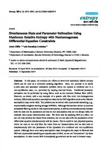
and the conditions in Theorem 1 hold. Finally, choose to satisfy (38). Then system (16)–(17) with the adaptive law (20) is well defined, and is an observer of system (47)–(48) in coordinates. For simulation purposes, the control signal is chosen as and the parameter . The initial or conditions are chosen as as in [11] and . The delay is chosen as and the initial value associated with the delay is chosen as . Fig. 1 shows the estimates for the system states and the parameter. The simulation results show the effectiveness of the proposed approach. Remark 7: Note that the term (19) appearing in the observer (16)–(18) is discontinuous which may result in chattering. In the simulation, the discontinuous function (19) has been replaced by the saturation function to avoid chattering [5]. It should be

1028


where

. Then, it is only required to prove that is observable. By direct verification, it follows from (51) and (52) that for any complex number :

and thus for any complex number (53)

Fig. 1. Evolution of system states mates and (dashed line).

and parameter

(solid line) and the esti-

Since is observable and PHB rank test

is nonsingular, from the

(54)

noted that in the simulation example, the matrix is chosen as due to the term in (47), which may result in large gain in the adaptive law (20) when is very small. As is usual for practical implementation, physical limits on the available control would need to be incorporated. V. CONCLUSION In this technical note, a sliding mode observer with an update law has been proposed to estimate the system states and unknown parameters. Coordinate transformations are used to explore the system structure and the features of the sliding mode approach are fully used to reduce conservatism. Both parametric uncertainty and structural uncertainty are considered. The system plant and the derived error dynamical system are time delayed and nonlinear. Furthermore, the unknown parameters are embedded in the system in a nonlinear fashion. The developed results is applicable to a wide class of systems.

Again, from the PHB rank test, (54) implies that the matrix pair is observable. Hence the conclusion follows. Let . A convex set associated with and is defined by

which is a subset in . Lemma 2: Let and the function . Then for any for

where is differentiable in for and , there exists such that

(55) represents a

where the notation by

function matrix defined

APPENDIX Consider a matrix pair where , and is full row rank with . The following result can be obtained. is observable and the matrix Lemma 1: If a matrix pair is full row rank, then there exists a nonsingular matrix such that

(56) where for

(50)

. Proof: From the multi-variable differential Mean Value Theorem, and , there exists it follows that for any such that

, the matrix is nonsingular where and is observable. Proof: From the fact that is full row rank, there exists a nonsuch that singular matrix (51) where way with

is nonsingular. Partition in (51) as

in a compatible

(52)

(57) where the point as well.

depends not only on

Let other terms as 0. Then

and

, but on

which has the -th entry as 1 and all

(58)


1029

Optimal Filtering for Discrete-Time Linear Systems With Multiplicative White Noise Perturbations and Periodic Coefficients

Substituting (57) into (58) yields

Vasile Dragan where

is defined in (55). Hence the conclusion follows.

REFERENCES [1] Y. Y. Cao and P. M. Frank, “Stability analysis and synthesis of nonlinear time-delay systems via linear Takagi-Sugeno fuzzy models,” Fuzzy Sets Syst., vol. 124, no. 2, pp. 213–229, 2001. [2] M. Chen and C. Chen, “Robust nonlinear observer for Lipschitz nonlinear systems subject to disturbance,” IEEE Trans. Automat. Control, vol. 52, no. 12, pp. 2365–2369, 2007. [3] L. Dugard and E. I. Verriest, Stability and Control of Time-Delay Systems (Lecture Notes in Control and Infromation Sciences 228). London, U.K.: Springer-Verlag, 1998. [4] D. Efimov and L. Fridman, “Global sliding-mode observer with adjusted gains for locally Lipschitz systems,” Automatica, vol. 47, no. 3, pp. 565–70, 2011. [5] F. Esfandiari and H. K. Khalil, “Stability analysis of a continuous implementation of variable structure control,” IEEE Trans. Automat. Control, vol. 36, no. 5, pp. 616–620, May 1991. [6] E. Fridman, A. Seuret, and J. Richard, “Robust sampled-data stabilization of linear systems: An input delay approach,” Automatica, vol. 40, no. 8, pp. 1441–1446, 2004. [7] A. Germani, C. Manes, and P. Pepe, “A new approach to state observation of nonlinear systems with delayed output,” IEEE Trans. Automat. Control, vol. 47, no. 1, pp. 96–101, Jan. 2002. [8] E. M. Jafarov, “Design modification of sliding mode observers for uncertain MIMO systems without and with time-delay,” Asian J. Control, vol. 7, no. 4, pp. 380–392, 2005. [9] E. M. Jafarov, “Robust sliding mode controllers design techniques for stabilization of multivariable time-delay systems with parameter perturbations and external disturbances,” Int. J. Syst. Sci., vol. 36, no. 7, pp. 433–444, 2005. [10] E. M. Jafarov, “Robust reduced-order sliding mode observer design,” Int. J. Syst. Sci., vol. 42, no. 4, pp. 567–577, 2011. [11] M. I. Neria-González, A. R. Domínguez-Bocanegra, J. Torres, R. Maya-Yescas, and R. Aguila-López, “Linearizing control based on adptive observer for anaerobic continuous sulphate reducing bioreactors with unknown kinetics,” Chem. Biochem. Eng. Quarterly, vol. 23, no. 2, pp. 179–185, 2009. [12] Y. Niu, J. Lam, X. Wang, and D. Ho, “Observer-based sliding mode control for nonlinear state-delayed systems,” Int. J. Syst. Sci., vol. 35, no. 2, pp. 139–150, 2004. [13] R. V. Patel and M. Toda, “Quantitative measure of robustness for multivariable systems,” in Proc. Joint Automat. Control Conf., TP8-A, San Francisco, CA, 1980, [CD ROM]. [14] A. M. Pertew, H. J. Marquez, and Q. Zhao, “H observer design for Lipschitz nonlinear systems,” IEEE Trans. Automat. Control, vol. 51, no. 7, pp. 1211–1216, Jul. 2006. [15] J. P. Richard, “Time-delay systems: An overview of some recent advances and open problems,” Automatica, vol. 39, no. 10, pp. 1667–1694, 2003. [16] Y. Shen, Y. Huang, and J. Gu, “Global finite-time observers for lipshitz nonlinear systems,” IEEE Trans. Automat. Control, vol. 56, no. 2, pp. 418–424, Feb. 2011. [17] S. K. Spurgeon, “Sliding mode observers: A survey,” Int. J. Syst. Sci., vol. 39, no. 8, pp. 751–764, 2008. [18] Ø. N. Stamnes, O. M. Aamo, and G.-O. Kaasa, “Adaptive redesign of nonlinear observers,” IEEE Trans. Automat. Control, vol. 56, no. 5, pp. 1152–57, May 2011. [19] X. G. Yan and C. Edwards, “Robust sliding mode observer-based actuator fault detection and isolation for a class of nonlinear systems,” Int. J. Syst. Sci., vol. 39, no. 4, pp. 349–59, 2008. [20] X. G. Yan, S. K. Spurgeon, and C. Edwards, “Sliding mode control for time-varying delayed systems based on a reduced-order observer,” Automatica, vol. 46, no. 8, pp. 1354–62, 2010. [21] Q. Zhang, “Adaptive observer for multiple-input-multiple-output (MIMO) linear time-varying systems,” IEEE Trans. Automat. Control, vol. 47, no. 3, pp. 525–529, Mar. 2002.

Abstract—In this technical brief, the problem of the estimation of a remote signal generated by a discrete-time dynamical system with periodic coefficients subject to multiplicative and additive white noise perturbations is investigated. To measure the quality of the estimation achieved by an admissible filter, we introduced a performance criterion described by the Cesaro limit of the mean square of the deviation between the estimated signal and the remote signal . The dimension of the state space of the admissible filters is not prefixed. The state-space representation of the optimal filter is constructed based on the unique periodic solution of a discrete-time linear equation together with the stabilizing solution of a suitable discrete-time Riccati equation with periodic coefficients. Index Terms—Discrete-time Riccati equations, discrete-time stochastic systems, multiplicative and additive white noise perturbations, periodic coefficients, signal filtering.

I. INTRODUCTION The estimation of a remote signal when measurements of another observed signal are available is a classical problem. Usually, both the remote signal and the measured signal are outputs of a dynamic system. In the case when the two signals are linear combinations of the states of a dynamic linear system, a significant advanced in the estimation problem was achieved by the Kalman-Bucy filter [14], [15]. In this case, both the system describing the evolution of the states as well as the measured output are assumed to be corrupted only by additive noise. An important issue in the Kalman type filtering intensively investigated over the last few decades is the influence of the modelling uncertainty of the plant which generates the remote signal over the filtering performance. Among the works devoted to the robust filtering for systems subjected to parametric uncertainty one mentions, for example, [17] and its references. Besides the deterministic representations of the model uncertainties there are many other cases when the plant parameters variations can be described as random perturbations of their nominal values. The stochastic systems have been intensively studied over the last four decades and many useful theoretical results including stability, robust design and optimal control are available (see e.g., [18] and [9]). The filtering problem for discrete-time linear stochastic systems with multiplicative white noise perturbations was investigated in [4]–[6], [10]. In [7], [8], [19] the estimation problem was considered for a wider class of linear stochastic systems. We refer to linear stochastic systems with Markovian jumping of the coefficients and affected by multiplicative and additive white noise perturbations. Lately, there is an increasing interest regarding the various control problems for time varying systems with periodic coefficients. A convincing motivation concerning the arising of the mathematical models described by equations with periodic coefficients together with a rich list of references related to this topic, may be found in the monographs [1], [12]. Our goal is to extend the results proved in [1, Chapter 12] to the case of systems having the state-space representation described by systems of discrete-time stochastic equations with periodic coefficients affected by Manuscript received August 11, 2011; revised April 01, 2012 and August 2, 2012; accepted August 15, 2012. Date of publication August 24, 2012; date of current version March 20, 2013. This work was supported by CNCS Romania under Grant 145/2011. Recommended by Associate Editor H. Zhang. The author is with the Institute of Mathematics “Simion Stoilow”, Romanian Academy, RO-014700 Bucharest, Romania (e-mail: [email protected]; [email protected]). Digital Object Identifier 10.1109/TAC.2012.2215534

0018-9286/$31.00 © 2012 IEEE