Copyright © 2002 IFAC 15th Triennial World Congress, Barcelona, Spain
TWO-STEP PARAMETER AND STATE ESTIMATION OF THE ANAEROBIC DIGESTION V. Lubenova, I.Simeonov*, I.Queinnec** Institute of Control and System Research, Bulgarian Academy of Sciences Acad. G. Bontchev St., Bock 2, 1113 Sofia, Bulgaria E-mail:
[email protected] *Institute of Microbiology, Bulgarian Academy of Sciences, Acad.G. Bonchev St., Block 26, Sofia 1113, Bulgaria E-mail:
[email protected] ** Laboratoire d'Analyse et d'Architecture des Systèmes (LAAS/CNRS) 7, Avenue du Colonel Roche, 31077 Toulouse cedex 4, France E-mail:
[email protected] Abstract: This paper is devoted to the state and parameter observation for anaerobic digestion process of organic waste. The observation has a two-step structure using separation of acidogenic stage from the methanogenic phase. Two observers and one estimator are built on the basis of a mass-balance nonlinear model of the process, involving a new control input, which reflects the addition of a stimulating substance (acetate). Laboratory experiments have been done with step changes of this new input. The stability of the observers is proven and performances are investigated on experimental data and simulations. Copyright© 2002 IFAC Keywords: anaerobic digestion, lab-scale experiments, acetate supply, non-linear model, parameter and state observation. 1. INTRODUCTION In the biological anaerobic wastewater treatment processes (methane fermentation) the organic matter is mineralised by microorganisms into biogas (methane and carbon dioxide) in absence of oxygen. The biogas is an additional energy source and the methane is a greenhouse gas. In general these processes are carried out in continuous stirred tank bioreactors (CSTR). Anaerobic digestion has been widely used in life process and has been confirmed as a promising method for solving some energy and ecological problems in agriculture and agro-industry. Mathematical modelling represents a very attractive tool for studying this process (Angelidaki, et al., 1999; Bastin and Dochain, 1991), however a lot of models are not appropriate for control purposes due to their complexity. The choice of relatively simple models of this process, their calibration (parameters and initial conditions estimation) and design of software sensors for the unmeasurable variables on the basis of an appropriate model are a very important steps for realization of sophisticated control algorithms (Bastin and Dochain, 1991; Cazzador and Lubenova, 1995; Lubenova, 1999; van Impe, et al., 1998).
The aim of this paper is twofold: -to calibrate the 4th order non-linear model of the methane fermentation with addition of a stimulating substance which may be viewed as control input (influent acetate concentration or acetate flow rate); -using two measurable process variables to design estimators of the growth rates and observers of the concentrations of the two main groups of microorganisms (acidogenic and methanogenic), appropriate for future control purposes.
2. PROCESS MODELLING 2.1. Experimental Studies Laboratory experiments hase been carried out in a 3-liter glass vessel CSTR bioreactor with highly concentrated organic pollutants (animal wastes) at mesophillic temperature and addition of acetate in low concentrations (mixed with the effluent organics and pH regulation of the added substrate) (Simeonov and Galabova, 1998). The tank is mechanically stirred by electrical drive and maintained at a constant
o
temperature 34±0.5 C by computer controller. The monitoring of the methane reactor is carried out by data acquisition computer system of on-line sensors, which provide the following measurements: pH, temperature (t o), redox, speed of agitation (n) and biogas flow rate (Q). The responses of Q are obtained for step changes of the acetate addition. The reported data offer the suggestion that acetate positively affects the methane production (when pH is in the admissible range) and increased levels of acetate as electron donor result in faster rates of methanogenesis.
2.2. Model of the Process On the basis of the above-presented experimental investigations and following the so-called two-stage biochemical scheme of the methane fermentation (Bastin and Dochain, 1991), the following 4th order nonlinear model with two control inputs is proposed (Simeonov and Galabova, 1998): dX 1 = (µ 1 − D )X 1 dt dS 1 = − k 1µ 1 X 1 + D1 S 'o − DS 1 dt dX 2 = (µ 2 − D )X 2 dt
(1)
dS 2 = dt
(4)
(2)
- k 2 µ 2 X 2 + k3 µ 1 X 1 + D2 S "o - DS 2
(5)
For the non-linear functions µ1 and µ2 the following structures are adopted: 1
=
µ max 1 S k
S1
+S
1
;
2
1
µ max2S
µ = k S2
≤ S 0' ≤ S 0'
inf
sup
(7)
2.3. Parameter Identification A sensitivity analysis with respect to nine coefficients was made only on the basis of simulation studies and they were divided into the following two groups: k1÷ k4 in the first group, µmax1, µmax2, ki2, ks1 and ks2 in the second group. Applying the methodology from (Simeonov, 2000) estimation starts with the first (more sensitive) group of coefficients with known initial values of all coefficients using optimisation method; estimation of the second group of coefficients with the above determined values of the first group is the following step, etc. Experimental data were given by measurements of S 2 and Q, with given conditions " S 0' , S 0 , D1 and D2. Results are summarised in Table 1. Table 1. Values obtained for the coefficients of the 4th order model with acetate addition µmax1 µmax2 0.2 0.25
ks1 0.3
ks2 0.87
k1 6.7
k2 4.2
k3 5
k4 4.35
ki2 1.5
(3)
Q = k4 µ 2 X 2
µ
0 ≤D ≤ Dsup; S 0'
2
,
(6)
2 +S + S / k 2 2 i2
where X [g/l], S[g/l], µ[day-1] are the bacteria concentration, the associated substrate concentration and the specific growth rate, respectively and Q[l/day] is the biogas flow rate. Indices 1 and 2 stand for the acidogenic and the methanogenic phases respectively. k1, k2, k3, k4[l/g], µmax1[day-1], µmax2[day-1], ks1[g/l], ks2[g/l], ki2 [g/l] are coefficients, D1 [day-1] is the dilution rate for the inlet soluble organics with concentration -1 S 0' [g/l], D2 [day ] is the dilution rate for the inlet acetate with concentration S 0" [g/l] and D=D1+D2 is the total dilution rate.
S 0' is generally an unmeasurable perturbation (on line),
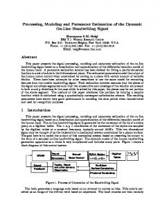
Some experimental and simulation results are compared on Fig.1 in the following conditions: D1 = 0.0375=const., D2 = 0.0125=const., S 0' =7.5 and S 0" =25 from t = 0 to 6;
S 0" =50 from t = 7 to 16; S 0" =75 from t = 17 to 35. Experimental data for D2=0.0125 with the first step change of S 0" have served for parameter estimation with initial values of the estimated parameters obtained from other experiment without acetate additation (D2=0). (Simeonov, 2000). Experimental data for D2=0.0125 with the 2nd and 3rd step changes of S 0" were used for model validation. It is evident the behavior of the model with the new control input is satisfying comparing to the process one. 1.6 Qexp
1.4 1.2
X1
1 0.8 Q
while Q and S 2 are measurable outputs, D1 and D2 are control inputs and S "0 is a known constant or control
0.6
input. In all cases the washout of microorganisms is undesirable, that is why changes of the control input D and the perturbation S 0' are possible only in some
0.2
admissible ranges (for fixed value of S "0 ):
Fig.1. Evolution of X1, X2, S 1, S 2, Q and Qexp in the case of step addition of acetate
5 S1
0.5 S2
0.4 0.1 X2 0
5
10
15 20 Time (days)
25
30
where Rˆ 1 is the estimate of R1 obtained by estimator 3. STATE ESTIMATION
(8), while the µ1 estimate can be derived on the basis of relationship:
3.1. Problem Statement
µˆ 1 m = Rˆ 1 / Xˆ
For the model (1)-(7) it is assumed that: A1. The growth rate R1 = µ1X1 associated to acidogenic bacteria, is unknown time-varying parameter, which is nonnegative and bounded, with bounded time derivative. A2. The concentrations of X1, X2, S 1, cannot be measured on-line, while methane production rate Q and substrate concentration S 2, are measured on-line. For the model (1)-(7) under the assumptions A1-A2, the following problem is considered: design an estimator of the growth rate R1 and observers of the concentrations X1 and X2, using on-line measurements of Q and S 2. The estimation approaches proposed by Bastin and Dochain (1990) cannot be applied for the considered bioprocess.
3.2 Indirect State and Parameter Estimation The indirect estimation is a simple method for restore of state and parameters, using process models: diferential equations or (and) kinetic models.
3.3. Estimator and Observer Design for the Acidogenic Stage Estimator of the growth rate R1 ; We assumed that: A3. Noisy measurements Qm and S 2m are available online: Qm=Q+ε1;
S 2m=S 2+ε2,
where ε1 and ε2 are measurements noises. The following observer-based estimator of R1 is proposed using the dynamical equation (4) of S 2 concentration: dSˆ2 = −DS2 m + k3 Rˆ1 − k2 R2 m dt , + D S " + C (S − Sˆ ) 2 0
1R 1
2m
(8)
Stability Analysis; Consider associated to the observer (8): dx dt
= Ax
+ u
~ S
S
x =
~ R
2
=
R 1
Dε
2
C 1R 1ε
1
ε
+ k
2 k
u = −
2
2
error
system (11)
Sˆ
-
Rˆ
-
1 − 4
dR +
the
2
;
-C A = -C
1
C 1R 1ε
2
1R1 2R1
k
3
;
0
,
1
dt
where x is the estimation error vector, u is the input vector of the error system and A is the matrix of the error system. The values of C1R1 , C 2R1 have to be chosen such that matrix A remains stable, i.e., C1R1 > 0 and C2R1 > 0. Observer of X1; To improve the convergence rate and consequently the estimation accuracy, a “software sensor” of X1 is derived. The proposed estimation algorithm can be considered as a modification of the observers proposed in (Dochain, 1986) concerning cases when the estimated variable is not observable from measurements. The dynamics of S 2 (4) is considered and the following auxiliary parameter is defined: ϕ1=R1+λ1 X1,
(12)
where λ1 is a bounded positive real number. Substituting R1 from (12) in the dynamical equation of S 2 (4), the following observer of X1 is derived: dSˆ2 = −DS2m + k3 ϕˆ1 − k3λ1 Xˆ 1 − k2R2m + D2S"0 + C1X 1(S2m − Sˆ2) dt (13) dXˆ1 =ϕˆ1 − (D + λ1)Xˆ1 +C2X1(S2m − Sˆ2) dt d ϕˆ1 = C3X1(S2m − Sˆ2) dt
2
where C1X1 , C2X1 C3X1 are observer parameters.
dRˆ1 = C2 R1 ( S2 m − Sˆ2 ) dt
where R2m=Qm/k4 = R2 +ε1/k4 are measured values of R2, ε1/k4 represents a measurement noise of R2 and C1R1, C2R1 are estimator parameters. The X1 estimates are obtained by: & Xˆ 1 m = Rˆ 1 − D Xˆ
(10)
1m
1m
(9)
More accurate estimates of the specific growth rate µ1 (in comparison with those derived from (10)) can be obtained using the kinetic model: µˆ 1 = Rˆ 1 / Xˆ
1
,
(14)
where Rˆ 1 are the estimates of R1 obtained from (8), while Xˆ 1 are the estimates of X1, obtained by observer (13).
Stability Analysis; Consider the dynamics of the estimation error (11). In the considered case, the values of the matrix and vectors are:
x =
~ S 2 ~ X 1 ϕ~
− C A = − C −
C
1
− λ k
1X1
1
2X1
− λ
1
0
3X1
− C 1X1 ε 2 − D ε 2 u = − C 2X1 ε 2 − C 3X1 ε 2 + ϕ& 1
k
3
− D
3
;
1
According the assumptions A6, A7, this function is positive and non-decreasing. Therefore, the exponential stability of the unforced part of the system (15) follows from theorems 9.9-9.11 (Hsu and Meyer, 1972). 2. The forcing term of the error system (11), (15) is bounded in the following way: − C1X1 ε 2 − Dε 2 − k2ε 3
0
u = − C2X1 ε 2
− k 2ε 3 ,
− C1X1 M 2 − DM2 − k 2M 3