State-Slice: New Paradigm of Multi-query Optimization of. Window-based Stream Queriesâ. Song Wang, Elke Rundensteiner. Worcester Polytechnic Institute.
State-Slice: New Paradigm of Multi-query Optimization of ∗ Window-based Stream Queries Song Wang, Elke Rundensteiner
Samrat Ganguly, Sudeept Bhatnagar
{songwang|rundenst}@cs.wpi.edu
{samrat|sudeept}@nec-labs.com
Worcester Polytechnic Institute Worcester, MA, USA.
NEC Laboratories America Inc. Princeton, NJ, USA.
ABSTRACT
query based applications involving a large number of concurrent queries over high volume data streams are emerging in a large variety of scientific and engineering domains. Examples of such applications include environmental monitoring systems [2] that allow multiple continuous queries over sensor data streams, with each query issued for independent monitoring purposes. Another example is the publish-subscribe services [7, 20] that host a large number of subscriptions monitoring published information from data sources. Such systems often process a variety of continuous queries that are similar in flavor on the same input streams. Processing each such compute-intensive query separately is inefficient and certainly not scalable to the huge number of queries encountered in these applications. One promising approach in the database literature to support large numbers of queries is computation sharing. Many papers [8, 18, 10, 13] have highlighted the importance of computation sharing in continuous queries. The previous work, e.g. [8], has focused primarily on sharing of filters with overlapping predicates, which are stateless and have simple semantics. However in practice, stateful operators such as joins and aggregations tend to dominate the usage of critical resources such as memory and CPU in a DSMS. These stateful operators tend to be bounded using window constraints on the otherwise infinite input streams. Efficient sharing of these stateful operators with possibly different window constraints thus becomes paramount, offering the promise of major reductions in resource consumption. Compared to traditional multi-query optimization, one new challenge in the sharing of stateful operators comes from the preference of in-memory processing of stream queries. Frequent access to hard disk will be too slow when arrival rates are high. Any sharing blind to the window constraints might keep tuples unnecessarily long in the system. A carefully designed sharing paradigm beyond traditional sharing of common sub-expressions is thus needed. In this paper, we focus on the problem of sharing of window join operators across multiple continuous queries. The window constraints may vary according to the semantics of each query. The sharing solutions employed in existing streaming systems, such as NiagaraCQ [10], CACQ [18] and PSoup [9], focus on exploiting common sub-expressions in queries, that is, they closely follow the traditional multiquery optimization strategies from relational technology [23, 21]. Their shared processing of joins ignores window constraints, even though windows clearly are critical for query semantics. The intuitive sharing method for joins [13] with different
Modern stream applications such as sensor monitoring systems and publish/subscription services necessitate the handling of large numbers of continuous queries specified over high volume data streams. Efficient sharing of computations among multiple continuous queries, especially for the memory- and CPU-intensive window-based operations, is critical. A novel challenge in this scenario is to allow resource sharing among similar queries, even if they employ windows of different lengths. This paper first reviews the existing sharing methods in the literature, and then illustrates the significant performance shortcomings of these methods. This paper then presents a novel paradigm for the sharing of window join queries. Namely we slice window states of a join operator into fine-grained window slices and form a chain of sliced window joins. By using an elaborate pipelining methodology, the number of joins after state slicing is reduced from quadratic to linear. This novel sharing paradigm enables us to push selections down into the chain and flexibly select subsequences of such sliced window joins for computation sharing among queries with different window sizes. Based on the state-slice sharing paradigm, two algorithms are proposed for the chain buildup. One minimizes the memory consumption while the other minimizes the CPU usage. The algorithms are proven to find the optimal chain with respect to memory or CPU usage for a given query workload. We have implemented the slice-share paradigm within the data stream management system CAPE. The experimental results show that our strategy provides the best performance over a diverse range of workload settings among all alternate solutions in the literature.
1.
INTRODUCTION
Recent years have witnessed a rapid increase of attention in data stream management systems (DSMS). Continuous ∗This work is funded in part by the NSF Computing Research Infrastructure grant CNS 05-51584 and NEC Laboratories America Inc.
Permission to copy without fee all or part of this material is granted provided that the copies are not made or distributed for direct commercial advantage, the VLDB copyright notice and the title of the publication and its date appear, and notice is given that copying is by permission of the Very Large Data Base Endowment. To copy otherwise, or to republish, to post on servers or to redistribute to lists, requires a fee and/or special permission from the publisher, ACM. VLDB ‘06, September 12-15, 2006, Seoul, Korea. Copyright 2006 VLDB Endowment, ACM 1-59593-385-9/06/09.
619
window sizes employs the join having the largest window among all given joins, and a routing operator which dispatches the joined result to each output. Such method suffers from significant shortcomings as shown using the motivation example below. The reason is two folds, (1) the per-tuple cost of routing results among multiple queries can be significant; and (2) the selection pull-up (see [10] for detailed discussions of selection pull-up and push-down) for matching query plans may waste large amounts of memory and CPU resources. Motivation Example: Consider the following two continuous queries in a sensor network expressed using an SQL-like language with window extension [2]. Q1: SELECT A.* FROM Temperature A, Humidity B WHERE A.LocationId=B.LocationId WINDOW 1 min Q2: SELECT A.* FROM Temperature A, Humidity B WHERE A.LocationId=B.LocationId AND A.Value>Threshold WINDOW 60 min Q1 and Q2 join the data streams coming from temperature and humidity sensors by their respective locations. The WINDOW clause indicates the size of the sliding windows of each query. The join operators in Q1 and Q2 are identical except for the filter condition and window constraints. The naive shared query plan will join the two streams first with the larger window constraint (60 min). The routing operator then splits the joined results and dispatches them to Q1 and Q2 respectively according to the tuples’ timestamps and the filter. The routing step of the joined tuples may take a significant chunk of CPU time if the fanout of the routing operator is much greater than one. If the join selectivity is high, the situation may further escalate since such cost is a per-tuple cost on every joined result tuple. Further, the state of the shared join operator requires a huge amount of memory to hold the tuples in the larger window without any early filtering of the input tuples. Suppose the selectivity of the filter in Q2 is 1%, a simple calculation reveals that the naive shared plan requires a state size that is 60 times larger than the state used by Q1 , or 100 times larger than the state used by Q2 each by themselves. In the case of high volume data stream inputs, such wasteful memory consumption is unaffordable and renders inefficient computation sharing. Our Approach: In order to efficiently share computations of window-based join operators, we propose a new paradigm for sharing join queries with different window constraints and filters. The two key ideas of our approach are: stateslicing and pipelining. We slice the window states of the shared join operator into fine-grained pieces based on the window constraints of individual queries. Multiple sliced window join operators, with each joining a distinct pair of sliced window states, can be formed. Selections now can be pushed down below any of the sliced window joins to avoid unnecessary computation and memory usage shown above. However, N 2 joins appear to be needed to provide a complete answer if each of the window states were to be sliced into N pieces. The number of distinct join operators needed would then be too large for a DSMS to hold for a large N . We overcome this hurdle by elegantly pipelining the slices. This enables us to build a chain of only N sliced window joins to compute the complete join result. This also enables us to selectively share a subsequence of such a chain of sliced
window join operators among queries with different window constraints. Based on the state-slice sharing paradigm, two algorithms are proposed for the chain buildup, one that minimizes the memory consumption and the other that minimizes the CPU usage. The algorithms are guaranteed to always find the optimal chain with respect to either memory or CPU cost, for a given query workload. The experimental results show that our strategy provides the best performance over a diverse range of workload settings among alternate solutions in the literature. Our Contributions: • We review the existing sharing strategies in the literature, highlighting their memory and CPU consumptions. • We introduce the concept of a chain of pipelining sliced window join operators, and prove its equivalence to the regular window-based join. • The memory and CPU costs of the chain of sliced window join operators are evaluated and analytically compared with the existing solutions. • Based on the insights gained from this analysis, we propose two algorithms to build the chain that minimizes the CPU or the memory cost of the shared query plan, respectively. We prove the optimality of both algorithms. • The proposed techniques are implemented in an actual DSMS (CAPE). Results of performance comparison of our proposed techniques with state-of-the-art sharing strategies are reported. Organization of Paper: The rest of the paper is organized as follows. Section 2 presents the preliminaries used in this paper. Section 3 shows the motivation example with detailed analytical performance comparisons of alternative sharing strategies of window-based joins. Section 4 describes the proposed chain of sliced window join operators. Sections 5 and 6 present the algorithms to build the chain. Section 7 presents the experimental results. Section 8 contains related work while Section 9 concludes the paper.
2.
PRELIMINARIES
A shared query plan capturing multi-queries is composed of operators in a directed acyclic graph (DAG). The input streams are unbounded sequences of tuples. Each tuple has an associated timestamp identifying its arrival time at the system. Similar to [6], we assume that the timestamps of the tuples have a global ordering based on the system’s clock. Sliding windows [5] are commonly used constraints to define the stateful operators. See [12] for a survey on windowbased join operations in the literature. The size of a window constraint is specified using either a time interval (timebased) or a count on the number of tuples (count-based). In this paper, we present our sharing paradigm using timebased windows. However, our proposed techniques can be applied to count-based window constraints in the same way. We also simplify the discussion of join conditions by using equijoin in this paper, while the proposed solution is applicable to any type of join condition. The sliding window equijoin between streams A and B, with window sizes W1 and W2 respectively over the common attribute Ci can be denoted as A[W1 ] 1Ci B[W2 ]. The semantics [24] for such sliding window joins are that the
620
denoted as λ. The analysis can be extended similarly for unbalanced input stream rates.
output of the join consists of all pairs of tuples a ∈ A, b ∈ B, such that a.Ci = b.Ci (we omit Ci in the future and instead concentrate on the sliding window only) and at certain time t, both a ∈ A[W1 ] and b ∈ B[W2 ]. That is, either Tb − Ta < W1 or Ta − Tb < W2 . Ta and Tb denote the timestamps of tuple a and b respectively in this paper. The timestamp assigned to the joined tuple is max(Ta , Tb ). The execution steps for a newly arriving tuple of A are shown in Fig. 1 1 . Symmetric steps are followed for a B tuple.
3.1
Naive Sharing with Selection Pull-up
The PullUp or Filtered PullUp approaches proposed in [10] for sharing continuous query plans containing joins and selections can be applied to the sharing of joins with different window sizes. That is, we need to introduce a router operator to dispatch the joined results to the respective query outputs. The intuition behind such sharing lies in that the answer of the join for Q1 (with the smaller window) is contained in the join for Q2 (with the larger window). The shared query plan for Q1 and Q2 is shown in Fig. 3.
1.Cross-Purge: Discard expired tuples in window B[W2 ] 2.Probe: Emit a 1 B[W2 ] 3.Insert: Add a to window A[W1 ]
Figure 1: Execution of Sliding-window join.
Q1
For each join operator, the input stream tuples are processed in the order of their timestamps. Main memory is used for the states of the join operators (state memory) and queues between operators (queue memory).
3.
Wi−1 , since Tb > Tb0 . We still have Tb − Tam > Wi−1 . Since Tam ≥ Tak , for ∀ak ∈ A :: [Wi−1 , Wi ], we have Wi−1 ≤ Tb − T ak , for ∀ak ∈ A :: [Wi−1 , Wi ]). (2). We use a proof by contradiction. If a ∈ / A :: [Wi−1 , Wi ], then first we assume a ∈ A :: [Wj−1 , Wj ], j < i. Given Wi−1 ≤ Tb − Ta , we know Wj ≤ Tb − Ta . Then a cannot be inside the state A :: [Wj−1 , Wj ] since a would have been purged by b when it is processed by the join operas tor A[Wj−1 , Wj ] n B. We got a contradiction. Similarly a cannot be inside any state A :: [Wk−1 , Wk ], k > i.
Fig. 7 shows a chain of state-sliced window joins having two one-way joins J1 and J2 . We assume the input stream tuples to J2 , no matter from stream A or from stream B, are processed strictly in the order of their global time-stamps. Thus we use one logical queue between J1 and J2 . This does not prevent us from using physical queues for individual input streams. Joined-Result Union U A Tuple
State of Stream A: [0, w1]
State of Stream A: [w1, w2] Queue(s)
B Tuple
Probe
Probe
J1
J2
Figure 7: Chain of 1-way Sliced Window Joins. Table 2 depicts an example execution of this chain. We assume that one single tuple (an a or a b) will only arrive at the start of each second, w1 = 2sec, w2 = 4sec and every a tuple will match every b tuple (Cartesian Product semantics). During every second, an operator will be selected to run. Each running of the operator will process one input tuple. The content of the states in J1 and J2 , and the content in the queue between J1 and J2 after each running of the operator are shown in Table 2. T 1 2 3 4
Arr. a1 a2 a3 b1
OP J1 J1 J1 J1
A :: [0, 2] [a1 ] [a2 ,a1 ] [a3 ,a2 ,a1 ] [a3 ,a2 ]
Queue [] [] [] [b1 ,a1 ]
A :: [2, 4] [] [] [] []
5 6 7 8 9 10
b2
J1 J2 J2 J1 J2 J2
[a3 ] [a3 ] [a3 ] [a4 ,a3 ] [a4 ] [a4 ]
[b2 ,a2 ,b1 ,a1 ] [b2 ,a2 ,b1 ] [b2 ,a2 ] [b2 ,a2 ] [a3 ,b2 ] [a3 ]
[] [a1 ] [a1 ] [a1 ] [a2 ,a1 ] [a2 ,a1 ]
a4
Theorem 1. The union of the join results of all the sliced s one-way window joins in a chain A[0, W1 ] n B, ..., A[WN −1 , s
WN ] n B is equivalent to the results of a regular one-way sliding window join A[WN ] n B.
Output
Proof: “⇐”. Lemma 1(1) shows that the sliced joins in a chain will not generate a result tuple (a, b) with Ta − Tb > s S W . That is, ∀(a, b) ∈ 1≤i≤N A[Wi−1 , Wi ] n B ⇒ (a, b) ∈ A[W ] n B. “⇒”. We need to show: ∀(a, b) ∈ A[W ]nB ⇒ ∃i, s.t.(a, b) ∈
(a2 ,b1 ), (a3 ,b1 ) (a3 ,b2 )
A[Wi−1 , Wi ] n B. Without loss of generality, ∀(a, b) ∈ A[W ]nB, there exists unique i, such that Wi−1 ≤ Tb −Ta < Wi , since W0 ≤ Tb − Ta < WN . We want to show that s (a, b) ∈ A[Wi−1 , Wi ] n B. The execution steps in Fig. 6
s
s
guarantee that the tuple b will be processed by A[Wi−1 , Wi ] n B at a certain time. Lemma 1(2) shows that tuple a would be inside the state of A[Wi−1 , Wi ] at that same time. Then
(a1 ,b1 ) (a1 ,b2 ), (a2 ,b2 )
s
(a, b) ∈ A[Wi−1 , Wi ] n B. Since i is unique, there is no duplicated probing between tuples a and b. From Lemma 1, we see that the state of the regular oneway sliding window join A[W ] n B is distributed among different sliced one-way joins in a chain. These sliced states are disjoint with each other in the chain, since the tuples in the state are purged from the state of the previous join. This property is independent from operator scheduling, be it synchronous or even asynchronous.
Table 2: Execution of the Chain: J1 , J2 . Execution in Table 2 follows the steps in Fig. 6. For example at the 4th second, first a1 will be purged out of J1 and inserted into the queue by the arriving b1 , since Tb1 −Ta1 ≥ 2sec. Then b1 will purge the state of J1 and output the joined result. Lastly, b1 is inserted into the queue. s Note that the union of the join results of J1 : A[0, w1] n B
4.2
s
and J2 : A[w1, w2] n B is equivalent to the results of a regular sliding window join: A[w2] n B. The order among the joined results is restored by the merge union operator. To prove that the chain of sliced joins provides the complete join answer, we first introduce the following lemma.
State-Sliced Binary Window Join
Similar to Definition 1, we can define the binary sliding window join. The definition of the chain of sliced binary joins is similar to Definition 2 and is thus omitted for space reasons. Fig. 8 shows an example of a chain of state-sliced binary window joins.
Lemma 1. For any sliced one-way sliding window join s A[Wi−1 , Wi ] n B in a chain, at the time that one b tuple finishes the cross-purge step, but not yet begins the probe step, we have: (1) ∀a ∈ A :: [Wi−1 , Wi ] ⇒ Wi−1 ≤ Tb − T a < Wi ; and (2) ∀a tuple in the input steam A, Wi−1 ≤ Tb − T a < Wi ⇒ a ∈ A :: [Wi−1 , Wi ]. Here A :: [Wi−1 , Wi ] denotes the state of stream A.
Definition 3. A sliced binary window join of streams A s and B is denoted as A[WAstart , WAend ] 1 B[WBstart , WBend ], where stream A has a sliding window of range: WAend − WAstart and stream B has a window of range WBend − WBstart . The join result consists of all pairs of tuples a ∈ A, b ∈ B, such that either WAstart ≤ Tb − Ta < WAend or WBstart ≤ Ta − Tb < WBend , and (a, b) satisfies the join condition.
Proof: (1). In the cross-purge step (Fig. 6), the arriving b will purge any tuple a with Tb − Ta ≥ Wi . Thus ∀ai ∈ A :: [Wi−1 , Wi ], Tb −T ai < Wi . For the first sliced window join in the chain, Wi−1 = 0. We have 0 ≤ Tb − T a. For other joins in the chain, there must exist a tuple am ∈ A :: [Wi−1 , Wi ] that has the maximum timestamp among all the a tuples in A :: [Wi−1 , Wi ]. Tuple am must have been purged by
The execution steps for sliced binary window joins can be viewed as a combination of two one-way sliced window joins. Each input tuple from stream A or B will be captured as two reference copies, before the tuple is processed by the first binary sliced window join2 . One reference is annotated as 2
623
The copies can be made by the first binary sliced join.
Joined-Result
as input tuples. The selection operator σA filters the input s 0 stream A tuples for 12 . The selection operator σA filters s the joined results of 11 for Q2 . The predicates in σA and 0 σA are both A.value > T hreshold.
U Union A Tuple
female
State of Stream A: [w1, w2]
State of Stream A: [0, w1]
male Queue(s) male B Tuple
female
State of Stream B: [0, w1]
State of Stream B: [w1, w2]
J2
Q2
Q1
J1
Figure 8: Chain of Binary Sliced Window Joins.
σ’A
the male tuple (denoted as am ) and the other as the female tuple (denoted as af ). The execution steps to be followed for the processing of a s stream A tuple by A[W start , W end ] 1 B[W start , W end ] are shown in Fig. 9. The execution procedure for the tuples arriving from stream B can be similarly defined.
U Union
A2
[W 1,W 2]
B2 s 2
[W 1,W 2]
σA A1
B1 s
[0,W 1]
When a new tuple am arrives 1.Cross-Purge: Update B[W start , W end ] to purge expired B tuples, i.e. if bf ∈ B[W start , W end ] and (Tam − Tbf ) > W end , move bf into the queue (if exists) towards next join operator or discard (if not exists) 2.Probe: Emit am join with bf ∈ B[W start , W end ] to JoinedResult queue 3.Propagate: Add am into the queue (if exists) towards next join operator or discard (if not exists)
1
A
[0,W 1]
B
Figure 10: State-Slice Sharing for Q1 and Q2.
4.3
Discussion and Analysis
Compared to alternative sharing approaches discussed in Section 3, the state-slice sharing paradigm offers the following benefits: • Selection can be pushed down into the middle of the join chain. Thus unnecessary probings in the join operators are avoided. • The routing cost is saved. Instead a pre-determined route is embedded in the query plan. • States of the sliced window joins in a chain are disjoint with each other. Thus no state memory is wasted. Using the same settings as in Section 3, we now calculate the state memory consumption Cm and the CPU cost Cp for the state-slice sharing paradigm as follows: (
When a new tuple af arrives 1.Insert: Add af into the sliding window A[W start , W end ]
Figure 9: Execution of Binary Sliced Window Join. Intuitively the male tuples of stream B and female tuples of stream A are used to generate join tuples equivalent s to a one-way join: A[W start , W end ] n B. The male tuples of stream A and female tuples of stream B are used to generate join tuples equivalent to the other one-way join: s A o B[W start , W end ]. Note that using two copies of a tuple will not require doubled system resources since: (1) the combined workload (in Fig. 9) to process a pair of female and male tuples equals the processing of one tuple in a regular join operator, since one tuple takes care of purging/probing and the other filling up the states; (2) the state of the binary sliced window join will only hold the female tuple; and (3) assuming a simplified queue (M/M/1), doubled arrival rate (from the two copies) and doubled service rate (from above (1)) still would not change the average queue size, if the system is stable. In our implementation, we use a copy-of-reference instead of a copy-of-object, aiming to reduce the potential extra queue memory during bursts of arrivals. Discussion of scheduling strategies and their effects on queues is beyond the scope of this paper.
Cm = Cp =
2λW1 Mt + (1 + Sσ )λ(W2 − W1 )Mt 2λ2 W1 + λ + 2λ2 Sσ (W2 − W1 )+ 4λ + 2λ + 2λ2 S1 W1
(3)
The first item of Cm corresponds to the state memory in s s 11 ; the second to the state memory in 12 . The first item of s Cp is the join probing cost of 11 ; the second the filter cost s of σA ; the third the join probing cost of 12 ; the fourth the cross-purge cost; while the fifth the union cost; the sixth the 0 . The union cost in Cp is proportional to the filter cost of σA input rates of streams A and B. The reason is that the male s tuple of the last sliced join 12 acts as punctuation [26] for the union operator. For example, the male tuple af1 is sent to the union operator after it finishes probing the state of s stream B in 12 , indicating that no more joined tuples with timestamps smaller than af1 will be generated in the future. Such punctuations are used by the union operator for the sorting of joined tuples from multiple join operators [26]. Comparing the memory and CPU costs for the different sharing solutions, namely naive sharing with selection pull-up (Eq. 1), stream partition with selection push-down (Eq. 2) and state-slice chain (Eq. 3), the savings of using the state slicing sharing are: 8 (1) (3) Cm −Cm (1−ρ)(1−Sσ ) > = > 2 (1) > Cm > > (2) (3) > C −C ρ m m > = 1+2ρ+(1−ρ)S < (2) σ Cm (1) (3) (4) Cp −Cp (1−ρ)(1−Sσ )+(2−ρ)S1 > = > 1+2S1 (1) > Cp > > (2) (3) > > Sσ S1 : Cp −Cp =
Theorem 2. The union of the join results of the sliced s binary window joins in a chain A[0, W1 ] 1 B[0, W1 ], ..., s A[WN −1 , WN ] 1 B[WN −1 , WN ] is equivalent to the results of a regular sliding window join A[WN ] 1 B[WN ]. Using Theorem 1, we can prove Theorem 2. Since we can treat a binary sliced window join as two parallel one-way sliced window joins, the proof is fairly straightforward. It is omitted here for space reasons. We now show how the proposed state-slice sharing can be applied to the running example in Section 3 to share the computation between the two queries. The shared plan is depicted in Figure 10. This shared query plan includes a s chain of two sliced sliding window join operators 11 and s s s 12 . The purged tuples from the states of 11 are sent to 12
(2) Cp
624
ρ(1−Sσ )+Sσ +Sσ S1 +ρS1
State-Slice over Selection-PullUp State-Slice over Selection-PushDown Memory Saving(%)
Join Selectivity=0.4 Join Selectivity=0.1 Join Selectivity=0.025
CPU Saving(%)
50
100
40
80
30
60
20
40
10
20
0
30 25 20 15 10 5 0
0 1
1
0.8 0
0.6 0.2
0.4 ρ=w1/w2
0.4 0.6
0.8
0.2
1
0.8 0
Selectivity Sσ
1 0
0.8
0.6 0.2
0.4 ρ=w1/w2
0.8
0.6
0
0.4 0.6
(a)
0.2
0.4 ρ=w1/w2
Selectivity Sσ
0.2 1 0
(b)
(i)
with Cm denoting Cm , Cp denoting Cp in Equation i (i = W1 , 0 < ρ < 1. 1, 2, 3); and window ratio ρ = W 2 The memory and CPU savings under various settings calculated from Equation 4 are depicted in Fig. 11. Compared to sharing alternatives in Section 3, state-slice sharing achieves significant savings. As a base case, when there is no selection in the query plans (i.e., Sσ = 1), state-slice sharing will consume the same amount of memory as the selection pullup while the CPU saving is proportional to the join selectivity S1 . When selection exists, state-slice sharing can save about 20%-30% memory, 10%-40% CPU over the alternatives on average. For the extreme settings, the memory savings can reach about 50% and the CPU savings about 100% (Fig. 11(a), 11(b)). The actual savings are sensitive to these parameters. Moreover, from Eq. 4 we can see that all the savings are positive. This means that the state-sliced sharing paradigm achieves the lowest memory and CPU costs under all these settings. Note that we omit λ in Eq. 4 for CPU cost comparison, since its effect is small when the number of queries is only 2. The CPU savings will increase with increasing λ, especially when the number of queries is large.
Selectivity Sσ
1 0
Selection PullUp; (c) CPU
N, w0 = 0). A union operator Ui is added to collect joined results from J1 , ..., Ji for query Qi (1 < i ≤ N ), as shown in Fig. 12. We call this chain the memory-optimal state-slice sharing (Mem-Opt). Q1
Q2
…
Q3
QN U Union
U Union U Union
A B
s
s
s
1
2
3
[0,w1]
[w1,w2]
[w2,w3]
…
s N
[wN-1,wN]
Figure 12: Mem-Opt State-Slice Sharing. The correctness of Mem-Opt state-slice sharing is proven in Theorem 3 by using Theorem 2. We have the following equivalence for i (1 ≤ i ≤ N ): Qi : A[wi ] 1 B[wi ] =
[
s
A[Wj−1 , Wj ] 1 B[Wj−1 , Wj ]
1≤j≤i
Theorem 3. The total state memory used by a Mem-Opt s chain of sliced joins J1 , J2 , ..., JN , with Ji as A[wi−1 , wi ] 1 B[wi−1 , wi ] (1 ≤ i ≤ N, w0 = 0) is equal to the state memory used by the regular sliding window join: A[wN ] 1 B[wN ]. Proof: From Lemma 1, the maximum timestamp difference of tuples (e.g., A tuples) in the state of Ji is (wi − wi−1 ), when continuous tuples from the other stream (e.g., B tuples) are processed. Assume the arrival rate of streams A and B is denoted by λA and λB respectively. Then we have:
STATE-SLICE: BUILD THE CHAIN
In this section, we discuss how to build an optimal shared query plan with a chain of sliced window joins. Consider a DSMS with N registered continuous queries, where each query performs a sliding window join A[wi ] 1 B[wi ] (1 ≤ i ≤ N ) over data streams A and B. The shared query plan is a DAG with multiple roots, one for each of the queries. Given a set of continuous queries, the queries are first sorted by their window lengths in ascending order. We propose two algorithms for building the state-slicing chain in that order (Section 5.1 and 5.2). The choice between them depends on the availability of the CPU and memory in the system. The chain can also first be built using one of the algorithms and migrated towards the other by merging or splitting the slices at runtime (Section 5.3).
5.1
0.2
0.8
…
5.
0.4 0.6
(c)
Figure 11: (a) Memory Comparison; (b) CPU Comparison: State-Slice vs. Comparison: State-Slice vs. Selection PushDown. (i)
Join Selectivity=0.4 Join Selectivity=0.1 Join Selectivity=0.025
CPU Saving(%)
P 1≤i≤N
= =
M emJi
(λA + λB )[(w1 − w0 ) + (w2 − w1 ) + ... + (wN − wN −1 )] (λA + λB )wN
(λA +λB )wN is the minimal amount of state memory that is required to generate the full joined result for QN . Thus the Mem-Opt chain consumes the minimal state memory. Let’s again use the count of comparisons per time unit as the metric for estimated CPU costs. Comparing the execution (Fig. 9) of a sliced window join with the execution (Fig. 1) of a regular window join, we notice that the probing cost of the chain of sliced joins: J1 , J2 , ..., JN is equivalent to the probing cost of the regular window join: A[wN ] 1 B[wN ]. Comparing to the alternative sharing paradigms in Section 3, we notice that the Mem-Opt chain may not always
Memory-Optimal State-Slicing
Without loss of generality, we assume that wi < wi+1 (1 ≤ i < N ). Let’s consider a chain of the N sliced joins: s J1 , J2 , ..., JN , with Ji as A[wi−1 , wi ] 1 B[wi−1 , wi ] (1 ≤ i ≤ 625
win since it requires CPU cost for: (1) (N − 1) more times of purging for each tuple in the streams A and B; (2) extra system overhead for running more operators; and (3) CPU cost for (N − 1) union operators. In the case that the selectivity of the join S1 is rather small, the routing cost in the selection pull-up sharing may be less than the extra cost of the Mem-Opt chain. In short, the Mem-Opt chain may not be the CPU-optimal solution for all settings.
5.2
v0
U Union
s
i
…
…
…