Exploring Change – A New Dimension of Data ... - VLDB Endowment

Exploring Change – A New Dimension of Data Analytics Tobias Bleifuß

Leon Bornemann

Theodore Johnson

Hasso Plattner Institute, University of Potsdam

Hasso Plattner Institute, University of Potsdam

AT&T Labs – Research

[email protected] Dmitri V. Kalashnikov

[email protected] Felix Naumann

AT&T Labs – Research

Hasso Plattner Institute, University of Potsdam

[email protected]

[email protected] Divesh Srivastava AT&T Labs – Research

[email protected]

[email protected] ABSTRACT

change, and while much technology has emerged to retrieve and analyze this data, there is not yet much research to explore and understand the nature of such change, i.e., the behavior of data and metadata, including schemata, over time. While such metadata change typically happens much less frequently, in our experience schemata are much less stable than what is alluded to in DBMS textbooks and what is desirable from a DB-admin’s or application developer’s point of view. Explicitly recognizing, exploring, and analyzing such change can reveal hidden properties, can alert to changes in data ingestion procedures, can help assess data quality, and can improve the analyses that data scientists conduct on the dataset over the time dimension. We define the problem of data change exploration as follows: For a given, dynamic dataset, efficiently identify, quantify, and summarize changes in data at (1) value-, (2) aggregate-, and (3) schema-level, and support users to effectively and interactively explore this change, as laid out in our short previous work [11]. Beyond the actual changed values, this problem definition includes such broad issues as (i) the fact that change occurred, (ii) the speed and frequency at which this change occurred, (iii) the source of the change, (iv) other values that experience similar change (in value) or correlated change (in time), or (v) reviewing the “history” of an entity. Each of these questions shall be answered at all three mentioned levels. In Section 4 we propose a more comprehensive list of possible exploration primitives relevant to a change exploration system. While there is much related work, which we discuss in the next section, none comes close to delivering what we propose. With this work we address a common but less studied addition to the well-known “V”s of big data [37]: To the common notions of volume, velocity, and variety that characterize big data problems, we address variability. While variety is typically viewed as differences in format, semantics and other properties between multiple data sources, we introduce variability as describing such differences even within a data source over time.

Data and metadata in datasets experience many different kinds of change. Values are inserted, deleted or updated; rows appear and disappear; columns are added or repurposed, etc. In such a dynamic situation, users might have many questions related to changes in the dataset, for instance which parts of the data are trustworthy and which are not? Users will wonder: How many changes have there been in the recent minutes, days or years? What kind of changes were made at which points of time? How dirty is the data? Is data cleansing required? The fact that data changed can hint at different hidden processes or agendas: a frequently crowd-updated city name may be controversial; a person whose name has been recently changed may be the target of vandalism; and so on. We show various use cases that benefit from recognizing and exploring such change. We envision a system and methods to interactively explore such change, addressing the variability dimension of big data challenges. To this end, we propose a model to capture change and the process of exploring dynamic data to identify salient changes. We provide exploration primitives along with motivational examples and measures for the volatility of data. We identify technical challenges that need to be addressed to make our vision a reality, and propose directions of future work for the data management community. PVLDB Reference Format: Tobias Bleifuß, Leon Bornemann, Theodore Johnson, Dmitri V. Kalashnikov, Felix Naumann, Divesh Srivastava. Exploring Change – A New Dimension of Data Analytics. PVLDB, 12(2): 85-98, 2018. DOI: https://doi.org/10.14778/3282495.3282496

1.

CHANGE IN DATA AND METADATA

Data change, all the time. This undeniable fact has motivated the development of database management systems in the first place. While they are good at recording this

1.1

This work is licensed under the Creative Commons AttributionNonCommercial-NoDerivatives 4.0 International License. To view a copy of this license, visit http://creativecommons.org/licenses/by-nc-nd/4.0/. For any use beyond those covered by this license, obtain permission by emailing [email protected]. Copyright is held by the owner/author(s). Publication rights licensed to the VLDB Endowment. Proceedings of the VLDB Endowment, Vol. 12, No. 2 ISSN 2150-8097. DOI: https://doi.org/10.14778/3282495.3282496

Use cases

Data change happens in very many different situations, and consequently there are many different use cases for the ability to explore such change, for example: Curiosity / exploration. For datasets of unknown content and unknown behavior, data exploration [18, 34] can help understand them, complementing any initial data pro-

85

Chicago’s infobox, which can be changed by anyone with an internet connection. Change exploration allows analysis of this value in various dimensions: First, we can consider all previous values – do they follow the expected gradual growth over the past years? Next, our proposed volatility measure can reveal what the expected change rate is for any population value of US cities – is Chicago’s updated at a similar frequency? Finally, we can measure the overall change frequency for all of Chicago’s infobox data – is it updated regularly at all? Scenario 1 shows how a user can detect value disagreement, which might decrease the trust in those values. At a more general level, we can distinguish several use cases, depending on the number of involved properties and entities. Table 1 shows six possible interpretations of observed changes in a short amount of time. For instance, a change of a single value for a single property might reflect a minor error correction. However, if many entities experience change in the same property, this might reflect a general reformatting of those values.

Table 1: Interpretation of temporally close value change-events. Value changes Same property Different properties Same entity Correction Update Two entities Relationship Causality Many entities Formatting Bulk- or periodic

filing [3] and analysis. The exploration of data changes adds another dimension to this process and can give insights that cannot be found in a static version of the dataset. All of our scenarios in Section 1.2 could be motivated by curiosity. Data production change / systemic change. Large applications today often consist of many diverse components and subsystems, connected via complex data flow graphs. Furthermore, some of the components can be independently developed by third parties. The output that such a component produces might occasionally undergo a systemic change: for instance, when the component is updated to a new version or certain parameters are changed. Results of a systemic change, for example, the way that one data stream in a subcomponent is collected, processed, and/or transported are well known to cause dramatic errors. These are often hard to debug when such a sweeping systematic change is unexpected by the rest of the application. Our vision entails the discovery of such systematic changes, with a small example shown in Scenario 3. Workload exploration. In cases where changes to a dataset are recorded, but the actual update statements/transactions are not, change exploration can help reverse engineer a sequence of data manipulation statements [25], identify reoccurring change instructions, and determine the general workload of the system [5]. Scenario 3 gives an example on how change exploration can help to assess the workload of a system and eventually reduce it. Change monitoring / change prediction. Observed patterns of data change can be used to predict occurrences of future changes [49] or change patterns [28], independent of the actual data values. Such models can be used to preallocate resources or to issue warnings when change does not occur as predicted. In Scenario 2, we explore schema changes that are likely to affect all entities of a certain type or class – a change monitoring system could alert if some entities were unexpectedly unaffected. Detecting errors in data and schema. Real-life data is often dirty and needs thorough cleaning [16, 17, 42] prior to further analysis. Particularly in crowd-sourced datasets, such as Wikidata, change exploration can reveal problems in the data values, such as vandalism [7] or sweeping, and thus likely accidental, deletes. We show examples of vandalism discovery in Scenario 1. In addition, changes can also be explored by property, attribute, or column. Classifying properties by their change behavior can uncover schema misuse or misplaced values. Building trust. For certain types of datasets, such as crowd-sourced or third party data, taking data at its face value can be a risky proposition. However, with the change history of the dataset, users can build trust [9]. As an example, consider infoboxes of Wikipedia pages, which contain a structured summary of the page’s most important facts. Now consider the value for the population of Chicago from

1.2

Motivating examples

To illustrate the usefulness and interestingness of change exploration, let us consider several scenarios for change exploration and analysis, which are relevant for multiple types of users. The first scenario on exploring value disagreement is interesting for DBAs, editors (users that update the data) and data quality engineers. The second scenario on schema change exploration and the fourth scenario on timecorrelated change-events give valuable insights to a data scientist, but the second one can also be of interest for a system designer because it can reveal past modeling decisions. For a DBA, the third scenario should be more interesting because it reveals information about dynamics and therefore necessary resource allocation and performance improvements.

1.2.1

Scenario 1: Explore value disagreement

For this and the next scenario, we consider exploring all changes made to Wikipedia’s infoboxes. These are usercurated, structured parts of Wikipedia pages. The base data for this scenario is provided by [7] and includes about 500 million change records, i.e., recorded changes of individual values, such as the insertion of a person’s shoe size or the change of a country’s population. In this scenario, an editor is interested in discovering topical controversies in Wikipedia [14], resulting in so-called edit-wars or even vandalism. Let us understand which exploration steps enable a user to discover parts of the dataset that suffer from such (unreasonably) frequent alterations. In the subsequent discussion, each underlined operator corresponds to a formal operator defined in Section 4, and maps to a simple interaction in our change exploration system. Because the user wants to determine whether settlement entities are affected by vandalism or edit wars, the user already filtered down the changes to actual updates (not initial inserts or final deletes) of settlement type. The discovered changes affect many different properties of settlements, such as population total and area code, which the user wants to distinguish. A split by property produces 849 separate change lists, one for each property. The user can now rank these lists by their volatility, a normalized measure of change frequency. Surprisingly, among the most volatile lists are those for the properties official name and name, which

86

100% 95%

among the data, which lists all properties in the order they appeared. Defining a ranking function to order by disappearance is more involved: To establish that a property has indeed disappeared, it must be verified that for each entity the last change is a deletion. For those, the ranking function returns the latest date of such a deletion, otherwise it returns the current date. Combining appearance and disappearance, one can determine the lifetime of a property, and visualize them for further analysis by the user. Even more advanced ranking functions for sets of changes that are split on property can determine their usage skew over time or other time-series analytics. Of course, a proven method in exploratory tools is to simply plot the number of change-occurrences per day/week/month along a time-axis. If direct schema change information is available, such as a log of ALTER TABLE statements for a relational database, our model is able to explicitly capture and explore these changes with the same set of operators.

population_total

90%

population_as_of

o cial_name

85%

subdivision_name leader_name

80%

subdivision_name1

75%

subdivision_type

70% image_skyline

65% % of change

subdivision_type1

map_caption

55% 50%

settlement_type

image_map

mapsize

60%

image_caption website

population_density_km2 longs subdivision_type2

45% 40%

name

subdivision_name2

35% 30%

Others

25% 20% 15% 10% 5% 0% 6/2007

12/2007

6/2008

12/2008

6/2009 12/2009 Time (resolution: 1 month)

6/2010

12/2010

6/2011

12/2011

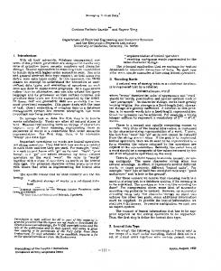
Figure 1: Distribution of the modified properties for settlements over time in the explored data set of Scenario 1. Surprisingly, two name attributes are among the 20 most frequently changed properties.

1.2.3 would be assumed to be quite stable. After all, the name of a city or town should not change very often, as opposed other properties, such as population. Figure 1 shows a visualization of these findings. Interested in which settlements experience such changes, the user now unions the two lists for official name and name and splits on entities, creating thousands of separate change lists, one for each settlement that experienced at least one renaming. Ranking by size reveals that the city of Chicago has experienced 328 name changes in its Wikipedia infobox with a total of 70 distinct names, including City of Chicago and City of Chicago, Illinois, but also City of Chicago(Home Of the Whopper) and Shlama Lama Ding Dong. Recognizing that most of these changes are mere vandalism, the user returns to the previous list of ranked properties and deliberately excludes properties expected to be mostly static. This action results in a new exploration branch, in which the user can continue exploring changes more likely to be genuine. In this way, prior work on controversy detection for Wikipedia [14] can be naturally supported at the level of its structured data. In general, such explorations can help users also detect vandalism and spam, and they are of course not limited to Wikipedia. By enabling users to explore the entire history of values, we empower them to judge whether the current values are trustworthy based on their own priors.

1.2.4 1.2.2

Scenario 3: Explore dynamics

In many cases, the relevancy or interestingness of a data item is related to the number of updates it experiences. Our framework allows to explore change frequency at various levels: Which entities experience the most changes (split by id and then rank by number of changes)? Which property is the most dynamic (split by property, slice by updates, and then rank by number of changes)? Which cell experiences the most changes? Etc. An analysis of these dynamics has already proven helpful in a production database: in this database, the majority of all updates (around 80%) in the entire database, were to a single table. In order to understand what was happening, the DBA had to design a custom temporal database of the table (which effectively encodes deltas on a per-row basis) and an ad-hoc analysis script. Through this analysis, the DBA found that 99% of the time the updates only affected a couple of fields. What is more, these fields were metadata fields, e.g., last-update timestamp, about the update. So the vast majority of updates to this database were overwriting existing values, and were useless. This database was struggling with its load, but these insights allowed to shed most of its update load by throttling this runaway update script. Our framework can support the DBA by systemizing such analyses, so that he or she is no longer dependent on such ad-hoc scripts and lucky findings.

Scenario 2: Explore schema changes

Scenario 4: Time-correlated change-events.

A more traditional use case is the discovery of changes in data that correlate in time. That is, the change of values in one property happens (frequently) in close time-proximity to changes in another property of the same entity (easy) or a different one. An underlying operation would be a traditional time-series mining operation to detect such significantly often re-occurring events. Our data-model can support this operation by providing not traditional (numeric) input values but the (Boolean) change events. For instance, when analyzing the change history of the Internet Movie Database (IMDB) we discovered clusters of change behavior based on the releases of series episodes [13]. The fact that our approach also allows analyzing changes from several sources simultaneously opens up further compelling analysis possibilities: for example, in this scenario the user can

Infobox templates guide Wikipedia authors and editors in creating property-value pairs. In particular, they are meant to ensure a common vocabulary of property names and thus increase infobox readability but also enable structured queries to the data. However, editors can change property names at will, some properties are hardly used, new properties appear. To maintain clean schemata and with it well-structured data, it is important to be able to identify both systematic and gradual changes in schema. A simple approach is to explore the appearance and disappearance of properties. A split of changes by property produces one change set per property. The data explorer can now use a pre-defined ranking function, for instance ranking by the date of the first appearance of the property

87

S1 ∆

S2 v5

… S9

log

Transforma -tion

behavior of a dataset. The change-cube can be physically stored in different representations, allowing traditional optimization techniques, such as indexing, materialized views, etc. The remainder of this vision paper is organized along the two major contributions (and challenges) of analyzing change: modeling change and exploring change. Section 3 (Modeling) introduces our central data structure, the changecube, and shows how to populate it and quantify change. Section 4 (Change Exploration Primitives) introduces the exploration primitives on top of the cube. Section 5 (Exploring) shows exemplary uses of our technology for a variety of initial use cases. Finally, Section 6 concludes our work with an outlook on the challenges to come. But first Section 2 discusses related work from various fields and in particular establishes the differences of change exploration to traditional time series analysis.

Web-based exploration & visualization

Data sources

Exploration primitives Fixed analytical queries (use-case specific)

Change Cube (virtual) Query translation

DBMS1

Change-mining methods (temporal outliers, …)

DBMS2

Figure 2: Architecture of a change exploration system. check whether changes take place first in the IMDB or first in Wikipedia and whether they propagate in one or the other direction and at what time offset. The necessity of a general change model is already evident from the fact that these two datasets exist in completely different data formats and that these data formats can also change over time for each data set. Furthermore, it would be necessary to develop specific change analysis tools for each data format, which we intend to solve with the following proposal for a general change model and analytical capabilities based on it.

1.3

2.

RELATED WORK

Because data change is a fundamental concept of databases, many research areas are related, though none come close to covering what we envision. In our work we want to explore not that data changes and how to react, but explore how, when, and where it changes. We leave the remaining traditional questions of who and why to future work. Traditional DBMS. With the technology to support transactions, triggers, versioning, logging, incremental view maintenance, etc., database systems include many methods to react to change. The rate of change is an area that is of particular importance to database optimization, in particular how they affect the statistics for query optimization [48,51]. Others have improved the when and how to rebuild the database statistics after data changes have occurred [48]. Our work aims far beyond these very specific statistics-based use cases to a general exploration of data change, and also includes change analysis at schema level. Temporal and sequence databases. Significant research and development efforts went into the design of databases or database extensions to support order-dependent queries [38] and temporal or sequence data [47]. For instance, SEQ is a system to support queries not over sets or multisets, but ordered collections of records [46]. Many later projects aim at further optimizing such queries and propose specialized query languages. At a finer grain, Dong et al. trace the value-history of individual entities by integrating multiple sources [22,23]. We formulate the combination of this integration aspect with our vision of exploring change for an entire, large dataset as a challenge in our final section. Lo et al. propose the “Sequence cuboid” which extends the traditional data cube with the concept of ordering [39]. The authors then extend SQL with sequence-specific operators, allowing, e.g., grouping by temporal patterns. Our proposal for modeling change (Section 3) is more general as it also captures schema change and explicitly targets the capture and analysis of change events rather than ordering a set of records. Our vision can certainly benefit from these previous ideas, which are mostly conceived for relational databases, but also exist, e.g., for graphs [35]. We plan to determine whether to adapt the techniques and insights to our more generic model

Structure and contributions

Given the motivation, use cases, and scenarios for change exploration, we can now formulate our first, overarching challenge. Challenge 1. How can we model and explore data and schema change for a variety of different input sources and for many different intended uses in an efficient and effective interactive fashion? Figure 2 shows an architectural overview of a change exploration system and serves as a guide for the remainder of the paper. The proposed system consumes data sources in various possible representations. Change of a dataset can be recorded in many different ways, such as transaction-logs, database differences as dump files, or timestamped snapshots of the entire database. Each of these variants must be consistently transformed into our general change representation: the central change-cube is our simple model to represent changes as quadruples of time, entity, property, and value. The change-cube is sufficiently generic to capture many different kinds of changes of data and schema from many different data models. And it is sufficiently expressive to serve a variety of change exploration use cases. We propose the change-cube as a first foundational step towards addressing Challenge 1. The remainder of the paper is based on this suggestion as a general model and the challenges that arise from it. On top of the change-cube we have defined a set of exploration primitives to slice, group, aggregate, sort, split and union sets of changes for further exploration. Many different clients can use these primitives. For instance, we have developed a web-based exploration tool to explore the cube, we have implemented clustering approaches to discover groups of similar changes, and we are able to define fixed analytical queries, for instance to monitor the change

88

of changes or to “outsource” specific analytical queries to such specialized systems. Temporal profiling. The general idea of adding a temporal dimension to database constraints and other metadata is not new. For instance, temporal association rules [6] are traditional association rules but defined over a (certain) time interval of certain length, during which it has particularly high support (or confidence). Jensen et al. formally define the extension of traditional dependencies, such as FDs or keys, to temporal databases [33]. We aim to provide a means to discover and explore such dependencies, supporting for instance web data cleaning [2]. Also, the Linked Data community has actively explored methods for the temporal analysis of linked data to understand the processes that populate the data sources [21] and to improve data services [50], or to explore ontological change [27]. The authors of [45] distinguish simple and userdefined complex changes in RDF datasets; our approach can discover complex changes at both data and schema level. Time series exploration. Exploration of time series data has been looked at by countless researchers [26], for instance to find similar time series [41,44]. These time series analysis techniques provide solutions for important parts of change exploration, such as obtaining stochastic models or identifying temporal update patterns. However, to use such techniques in our context, the research questions to be solved are how the database changes can be translated meaningfully to numerical time series and how the relevant time series for a certain problem can be selected. In addition, time series exploration techniques and tools [52] can be used to visualize and interpret change behavior. Data stream mining. A large body of work has proposed analytical methods on data streams [4]. The focus of these methods is mainly on (i) numeric data, (ii) a single dimension/attribute, and (iii) rapidly changing data. The goal is typically a prediction of values, based on past behavior, for instance to predict hardware failure or stock prices, or outlier and pattern detection. In contrast, we want to enable efficient ad-hoc exploration, we consider data, metadata, and time as equal dimensions, and do not constrain ourselves with the limitations of a streaming environment. Data and metadata exploration. With more and more relevant data available, the need to interactively explore it has been recognized. For instance, based on profiling results created by the Bellman tool [20], Dasu et al. have explored how data and schema changes in a database can be observed through a limited set of metadata [19]. That work has focused on the case of only limited access to the database. In contrast, we assume full access to the database and its changes, and are thus able to focus on more finegrained change exploration. But also in general, we plan to make use of the various recent visualization and interaction frameworks [31], to enable not only static analysis but interactive exploration of the nature of data change. Eichmann et al. go a step further and suggest an exploration benchmark [24]. Under their classification, our vision for an exploration system, as outlined in Section 5.2, would fall into the Categories I (interactive visual analysis) and III (recommendations). M¨ uller et al. have proposed the notion of update distance, i.e., “the minimal number of set-oriented insert, delete and modification operations necessary to transform one database

into the other.” [40]. While the authors propose to use this measure to compare drift among replicas, it could also be applied to compute the change rate of a database, for instance. However, the proposed algorithms to (even approximately) compute the update distance are tested only on toy examples and do not scale to real-world database sizes. Other notions of database distance are from the areas of consistent query answering [8] and minimal database repair [12], but both assume some given constraints, while our work is independent of any such constraints. Throughout this work we assume to have knowledge of the actual change of data in the given database, and want to explore the nature of this change. If that assumption does not hold, Inmon and Conklin point out three different ways to obtain this information [32]: Have the application explicitly report the change, parse the change from the logfile, or compute the difference between two snapshots of the database. Labio and Garcia-Molina tackled this last and difficult snapshot differential problem for table data [36] and Chawathe and Garcia-Molina for nested data [15]. Provenance / Lineage. Our vision certainly shares some common goals or use cases with data provenance [29]. Any information we have about the data provenance may certainly provide further input for our analysis and the provenance itself may become the subject of our change analysis. Despite this, we do not assume provenance information, but accept the changes as given. Furthermore, it could be possible to infer provenance information based on the observed changes. Just as change exploration can benefit from provenance, provenance analysis can also benefit from our work through a better understanding of source evolution. In summary, most related work in this area is concerned with capturing and managing data and database change, and not so much in exploring/understanding this change, leaving the following higher-level challenge open. Challenge 2. How can we leverage prior research in all areas that consider the temporal dimension of data to improve the change exploration experience?

3.

MODELING CHANGE

We introduce the change-cube as our central data structure to capture changes to both schema and data. First, we formally define the cube, and then illustrate the challenges of populating it from various types of data sources. Finally, we propose a volatility measure to quantify the degree of change to any element of the cube.

3.1

The Change-Cube

We propose a generic model to represent changes to a dataset. It includes the following four dimensions to represent when (time) what (entity) changed where (property) and how (new value): Time A timestamp in the finest available granularity. Entity The id of an entity represented in the dataset. An entity could correspond to a row in a relational database, a node in a graph, a subject of an RDF-triple, a schema element, etc. Entities can be grouped or belong to a hierarchy, modeled separately. In this way, we can recognize which rows belong to the same table, which RDF-subjects are of the same class, etc.

89

Property The property of the entity. Properties can be entities themselves and correspond to columns in a table, properties of a graph, predicates of an RDF-triple, schema associations, etc. Properties can be hierarchically organized, for instance grouped by semantic domain, such as person name, address, etc., or by datatype.

The model can record changes to the properties themselves, even their displayed names: h01.01.2012, property:size, property:displayname, ’area’i h01.01.2012, property:size, property:type, ’Double’i h17.02.2016, property:size, property:displayname, ’AREA:’i For space-efficiency, change-cubes can be implemented in a star-schema with a central fact-table containing only four numeric ids and dimension tables for each of the four dimensions. In some use cases, the value itself is not needed, only the fact that a change occurred. In such cases, further simplification/efficiency can be achieved by removing the value dimension or reducing it to the type of change or the severity of change that the value resembles. Further, in many real-world situations, additional data is available, such as the identity of the person or system that performed the change or a comment about the change. Such additions can be modeled within the change-cube if needed, but are not considered further here. The change-cube is different from the traditional data cube in three ways: First, instead of allowing a separate dimension for each property/attribute of the data, we gather them all into a single dimension, because we will be asking the same kind of questions for each attribute (namely change-related questions and not necessarily questions about the actual values). So for instance, instead of asking about an average value, we are asking about how often it changed over time or how often it appeared over time. In addition, we want to be explorative and easily add new properties to the model. For our Wikipedia infobox example, we can represent all 6,534 properties in this single dimension, instead of a sparse table of that width. Second, entities of various tables or classes are gathered into one cube; thus an attribute with a same name that is used across multiple tables (e.g., “address”) can have values at various sources but its changes can be explored summarily. Third, the domains of all properties are gathered into a (potentially very large) value-dimension. In this way, a value that appears in multiple locations across attributes (and tables) can be recognized as such. Thus, schema changes that were not explicitly captured, such as renaming attributes or tables, can be recognized.

Value The new value introduced by the change (or the nullvalue (⊥) to represent a deletion). Values can be literals, which we denote in quotes, or ids of other entities. Furthermore, values need not be atomic, they can be sets or lists. Without the time-dimension, the cube represents the traditional model-independent representation of facts as triples. By including time we can define an individual change and the change-cube as a set of changes: Definition 1. A change c is a quadruple of the form htimestamp, id, property, valuei or in brief ht, id, p, vi. We call a set of changes a change-cube C = {c1 , . . . , cn }. Among the changes, combinations of (t, id, p) are unique. The semantics of a change is: At time timestamp the property of the entity identified with id was created as or changed to value. A change can be used to express changes in data or in the schema. While we define the change-cube as a set, in many situations we shall order the changes. A “natural” ordering would be by timestamp, id, and property. This ordering is useful both from an exploratory perspective to orient users, and from an implementation perspective where a given order can be used to speed up various operators on the cube. We require that (timestamp, id, property) is a key, i.e., we do not allow multiple changes to occur for a single idproperty combination simultaneously. Without this assumption, a current state of the database would be ambiguous. In case of unreliable timestamps or time intervals [1], which can occur in practice, we assume a domain-dependent resolution of (order) conflicts. Further, we assume that id is a stable identifier throughout the lifetime of the representation of the entity. Without this assumption, the notion of “change” would be meaningless: each change-quadruple could be referencing an entirely new entity. Implicitly, a value of a change is valid from timestamp until the closest succeeding timestamp of a quadruple with same id and property but different value. Or it is valid until “now”, when no succeeding quadruple exists. To distinguish between changes to data and schema we use namespaces as prefixes to entities. As an example, consider the following change-cube:

3.2

Populating the change-cube

While all subsequent steps will profit by the unified changecube model, it entails the upfront overhead of transforming the changes into the change-cube. The obvious problem is that there are many different ways of how the changes are stored in the real-world, which implies a high variety of different input formats. Think of the extremes: the most finegranular input are individual transactions each with a precise timestamp. On the other side, we can also face the unfortunate case that only monthly (or even irregular) dumps of the entire database are available. In that case we must assume that all changes happened at once (at time of dump) and have to find a way to calculate the difference between two consecutive dumps, a problem highly dependent on the data model. Of course we can also imagine many different formats in between those extremes, such as timed database differences (patch files) or data logs, and each of these variants must be consistently transformed into the change-cube representation.

h01.01.2010, table:Persons, property:name, ’Person’i h01.01.2010, London, property:area, ’1,572km2 ’i The namespace table in the id of the first change signals that this change refers to a schema-element, whereas the second change refers to a data element. Namespaces are user-defined, but we have default suggestions, such as data, table, property, and others. In this paper we use meaningful names to denote properties and ids to increase readability.

90

Dealing with timestamps. Timestamps can have different granularities. For data that is inherently temporal, such as event data, we distinguish two kinds of “times” [47]:

work on transformation to RDF however, we face the additional problem that our data and also the schema is not static. For example, if a schema change deletes one of the columns that were part of the key, this will appear in the change-cube as if all entities were deleted and new entities were inserted. Instead, we want to recognize such cases and map the same entity always to the same key, although its key in the database can take different values over time. A complete lack of a key, e.g., in web tables, poses a similar problem and sometimes even multiple solutions make sense and a modeling decision needs to be made by the user. For example, consider a table of music charts: intuitively every album is represented by an entity that possesses a property chart-position. However, it is equally valid to model chart positions as entities with a property called album. For our model both approaches are valid, but it is clear that such decisions impact the results of subsequent analysis. Hierarchical data formats, such as JSON or XML, pose greater challenges than relational formats. Again, the user should make decisions on which representation makes most sense for further analysis. Generic transformations are also available, but these formats can contain collections, such as lists or arrays – and the position in a list is often a semantically uninformative and unstable choice for stable identification of entities. Consider the example of a book that has a list of authors. If the first two authors switch places, a trivial solution might assume that all details for both authors changed and fail to realize that only a property of the book (order of authors) has changed. But for other cases this might be the correct interpretation and once more, the answer depends on the use case. Because schema changes are also subject of our exploration, a transformation into the change-cube must not completely hide schema changes, so that schema change records also appear in the change-cube. It is not necessary to develop a transformation for each schema (which can vary over time within the same dataset), but rather to find a solution at the level of data models.

• Transaction time is the time when the change entered the database, optionally marked with a timestamp. • Valid time is the time recorded for a record and stored in the database. An example is the release date of an album. Sometimes the two coincide or are close to one another. In any given database, any combination of transaction time and valid time might be observable: Transaction time is often not recorded, because it may not be deemed important for the originally intended application. In some cases, transaction time can be recreated through transaction logs, through active monitoring of the database and storing observations on the side, or approximated using information about the order in which data entered the database (autoincrementing keys). During user interaction we have the choice of either type of time to be the assumed semantics of the timestamp dimension. The system should make every effort to record valid time as the timestamp. In its absence, the transaction time needs to suffice. In cases where a transaction id is present, we want to use it to populate or refine the timestamp dimension. To be able to distinguish transactions that have the same timestamp, there are several choices. We could suffix the timestamp with a transaction-id, with the disadvantage that we lose the timestamp datatype. Another option is to increase the timestamp granularity and divide up the transactions to multiple timestamps. This option has the disadvantage of creating fresh timestamps. In general, we are not able to know the true order of the change operations. Modeling decisions. For transforming input data to the change-cube there are two basic decisions to be made: what is the entity (id) and what is the property? These two decisions determine the value dimension. In general, entities need to be chosen fine enough to have preferably atomic properties, and coarse enough for it to exist long enough to observe its change. Properties should also be as persistent as possible, so long histories can be observed. The choice of what is an entity and what is a property is in general domain-dependent and also depends on the data format. However, there is a large corpus of literature on how to transform different data models into RDF, which faces the same basic problem. This literature also shows that our model is rich enough to express changes in any of those data formats. Database systems do offer further input to analyze and understand change, such as triggers, logs, and other constraints. However, we do not want to assume their presence and thus chose a more data-oriented approach. Based on new insights gained during the exploration, for instance after recognizing a previously unknown schema change, the user can introduce new views on the change-cube that capture the newly discovered knowledge. For relational data, a common assumption is that the entity is defined through the primary key of a table. If the key consists of multiple columns, we suggest to concatenate the values of these columns and separate them by a special character. The values of all other columns in a table correspond to the values of the properties, the property ids and names are given by the schema. In contrast to related

Challenge 3. How can we leverage research and tooling in the area of ETL to support users in creating semantically meaningful transformations beyond generic initial approaches?

3.3

A Measure for Volatility

Having modeled a dataset’s change in a change-cube, we now propose a very first measure to quantify change: Volatility measures the amount or degree of change of an object. In our context we want to assess the volatility of data at all levels by first counting the number of changes within a given time interval for (i) an entity-property combination, e.g., a field in a table, (ii) an entity across its properties, and (iii) a property across its entities, and then normalizing the count. To formally define a volatility measure, we must define precisely what we are counting and by which value we normalize. Counting the number of changes of the value of a particular field is trivial. But at any higher aggregation level (e.g., entity or property) we need to decide how to count changes in fields that no longer exist in the current version. To count the number of changes to a particular entity, we need to aggregate the number of changes to all values of its current properties, but also of all properties for

91

exampleVolatility Settlement area_code coordinates image_caption image_flag image_map Berlin 19 7 103 18 18 Cape Town 56 2 100 89 50 Chicago 235 5 290 475 472 Istanbul 100 3 294 6 4 51 439 London 116 1 554 Potsdam 5 1 24 3 4 Rome 245 32 141 324 324 12 Stockholm 20 1 46 10 Tokyo 135 15 166 156 156 Sum 931 67 1718 1132 1479

name population_as_of postal_code website 383 19 20 251 55 78 57 63 275 517 47 459 162 163 101 107 620 397 384 390 31 4 5 22 272 347 250 344 32 99 58 56 754 149 135 503 2584 1773 1057 2195

Sum 838 550 2775 940 2952 99 2279 334 2169 12936

Figure 3: A heatmap for changes on selected Wikipedia settlement entities and selected infobox properties, color-coded relative to the absolute number of changes. which it had values in the past. The same is true when measuring the volatility of a column: We need to consider all current entities that have that property, but also any entity that ever had that property (within the time interval under consideration). For ease of exposition, assume that data is represented as a relation with each tuple representing an entity and each attribute representing a property. The set of entities is the union of all entities that have been represented in a tuple in the table at some point. The set of properties is the union of all properties that have been defined for this table as an attribute. Let the pair hi, ji represent one field of this expanded relation where i designates the tuple and j the attribute.

value. For the latter case, for instance, we have observed the value Episode #1.1 to be particularly volatile in the IMDB dataset as the value of the title property. We assume that it represents a placeholder for TV-series before the final title is published. Changes could also be weighted by their severity before entering the count. For instance, a correction from the string Barak Obama to Barack Obama is less severe than one to Donald Trump. For numeric values, severity could be determined by a normalized difference, etc. Users are of course free to use custom volatility-measures. Challenge 4. How can we design and develop measures to flexibly encompass all aspects of change, such as change severity, datatype, time-intervals, change-origin, regularity, value-frequency, etc.? And how can we efficiently support the calculation of these measures?

Definition 2 (Volatility). For each field hi, ji let cij denote the number of changes that it has experienced P within the time interval under consideration. Let C = ij cij be the overall number of changes. We define the following volatility measures: • •

4.

c Field-volatility: v(hi, ji) = Cij P cij Entity-volatility: v(ei ) = jC P

• Property-volatility: v(pj ) =

CHANGE EXPLORATION PRIMITIVES

This section defines a set of operations on the change-cube that enable its fine-grained exploration. Our main contribution is to support human exploration of change. To mimic useful exploratory interactions of a user with change-cubes, we promote the cubes to be first class citizens and define a closed set of operators on sets of these cubes: sort to arrange the changes within a change-cube according to specific criteria, slice to specify subcubes, i.e., selected parts of an input change-cube; to create a set of change-cubes Pagesplit, 1 from an input change-cube; the union of two change-cubes to a single larger change-cube; and rank as well as prune to focus on change-cubes of interest, e.g., those with a high change-rate.

cij C

i

Figure 3 shows an exemplary use of volatility measures for a selection of cities and properties from their respective Wikipedia infoboxes (from the initial creation of the respective infobox until July 2017). The values correspond to the number of changes that each particular field experienced since the creation of the particular infobox. The colors are coded based on the respective volatilities. Already this small example shows several insights: As expected the coordinates of a city rarely change. But surprisingly, the names of the cities undergo frequent changes. For instance, the name of “Tokyo” has also been Tokio, Tokyo (Godzilla Central), ∅ and many offensive terms. Another observation is that the frequencies for the changes of flag- and map-images are almost always the same or very similar. And indeed, we can check that they are commonly changed together. Finally, and again as expected a smaller and less famous city like Potsdam experiences fewer value changes than larger or more well-known cities. The concept of volatility could be applied to various other elements in our change scenario. Examples include the volatility of a time interval in relation to (all) other time intervals, the volatility of an entire cube in relation to (all) other cubes, or (a bit more unusual) the volatility of a particular

4.1

Sort

While we earlier asserted a natural ordering of changes by timestamp, id, and property, it is of course possible to reorder the changes in other ways. We use square brackets to distinguish an explicitly ordered list from an unordered set. Definition 3 (sort). Given a change-cube C = {c1 , . . . , cn } and a function s : ht, id, p, vi 7→ z that maps a change to an atomic comparable value z, the ascending sort operator is defined as: sort↑s (C) := [ci1 , . . . , cin ] where ij ≤ ik if s(cij ) ≤ s(cik ) The descending sort operator sort↓s (C) is defined analogously.

92

• Split by time: Creates one list for each specified timeinterval (e.g., one list per year), for instance to discover regularly repeating change events.

To allow a fast and convenient exploration, we predefine four convenient functions that map changes to the value of each of the dimensions respectively: t : ht, id, p, vi 7→ t, p : ht, id, p, vi 7→ p,

id : ht, id, p, vi 7→ id,

In the most simple, exploratory form, the user simply specifies one of the four dimensions along which to split. The split then creates a change-cube for each distinct value present in that dimension of the input cube:

v : ht, id, p, vi 7→ v

These functions allow the user to write for example sort↑id to sort the changes by id. Still, more complex sorting, such as by the number of ‘a’s in a given property, is possible.

4.2

Definition 5 (split). Given a change-cube C and any split function s : ht, id, p, vi 7→ z that maps each change record to an atomic value z. Then

Slice

Each dimension of a cube can be the target of a selection operation, to reduce the change records to a list with a fixed value for one (or more) dimensions.

splits (C) := {slices(·)=x (C) | x ∈ range(s)} For a set of change-cubes C = {C1 , . . . , Cn } the split by a split function s is the union of each cube’s split: [ splits (C) := splits (C)

Definition 4 (slice). Given a change-cube C and a predicate q = ht, id, p, vi 7→ {true, false}. The slice operator is defined as:

C∈C

sliceq (C) := {x ∈ C | q(x) = true}

This definition includes simple splits by any dimension, e.g., by property through the already defined split function s : ht, id, p, vi 7→ p. But higher-level splits are also possible, e.g., a split by id-class, creates one cube per class or table (i.e., potentially hundreds of lists). Through a function such as s(ht, id, p, vi) := year(t), where year extracts the calendaryear of a given timestamp, a split by year creates one cube per year. When handling multiple change-cubes, it is useful to be able to combine them again into a larger change-cube. For instance, after a split the user might want to focus on analyzing all changes in a selected (e.g., top-K) subset of changecubes.

For a set of change-cubes C = {C1 , . . . , Cn } we define sliceq (C) := {sliceq (C1 ), . . . , sliceq (Cn )}. The most common form of predicates is q(x) = s(x) θ z, where θ is a built-in predicate, s : ht, id, p, vi 7→ z is a function that maps each change to an atomic, comparable value, and z is a constant of the same domain. For example the user could slice for all changes to the property population using the operator slicep=‘population’ . For slices on multiple predicates or in more than one dimension we apply successive slices. Thus in this simple case, each of these slices corresponds to a user clicking on an existing value of some change, and turning this value into a predicate. Slicing answers different questions in each dimension: What else happened with this entity? Which other entities and values of this property were changed? Where was this value also inserted? What else happened during this time? The predicates could also address a higher level of abstraction. For instance, one can specify a slice for a specific class of entities or a class of properties (or a type of value). The predicates need to rely on built-in operators, but could for example use a notion of similarity. A similarity in time is already present through the order. For instance, value-similarity could be based on edit-distance, propertysimilarity on data-type or domain, and entity-similarity based on class or high-level similarity measures from the research area of entity-resolution.

4.3

Definition 6. Given a set C of change-cubes, we define [ union(C) := C C∈C

4.4

Rank and prune

Splits often lead to a high number of change-cubes and therefore it is useful to give users a means to prioritize further investigation. One such tool is the ordering of changecubes, which can be based on various criteria: the size of the change-cube, its volatility, recency of the last change, the timespan between first and last change, etc. In addition, any user-defined rankings for custom definitions of interestingness are possible. Rankings are defined through an aggregate function o : C 7→ z, which maps each change-cube C to an atomic, comparable value z. A simple example would be o(C) := |C| to rank cubes by their size or o(C) := max(Πtimestamp (C)) − min(Πtimestamp (C)) to rank cubes by their covered time range.

Split and union

Given a change-cube, a split partitions/groups the changes into multiple sublists, according to the specified split condition. Again, each dimension can serve as a split-condition:

Definition 7 (rank). Given a set of change-cubes C = {C1 , . . . , Cm } and an aggregate function o, the rank operator is defined as:

• Split by id: Creates one list for each id (i.e., potentially millions of lists if done on an entire, unsliced cube), for instance to explore and compare how each entity of the dataset changes over time. • Split by property: Creates one list for each property (i.e., potentially thousands of lists) for instance to explore and compare the change of usage of properties and attributes over time. • Split by value: Creates one list for each value (i.e., potentially billions of lists), for instance to explore and compare the longevity of specific values.

ranko (C) := [Ci1 , . . . , Cin ] where ij ≤ ik if o(Cij ) ≤ o(Cik ) Ascending or descending order can be implemented by appropriate definitions of o(). Again, we use square brackets to distinguish an ordered list from an unordered set. To reduce the number of lists, a pruning based on the same aggregate functions is possible. For instance, a user may be interested only in the

93

5.

top-k change-cubes according to some ordering, or only in change-cubes such that the aggregate function complies with a threshold.

EXPLORING CHANGE

Definition 8 (prune). Given a descendingly ordered list of change-cubes C = [C1 , . . . , Cn ], the aggregate function o, and a threshold θ, we define the prune operator as the ordered list of change-cubes whose aggregate value is at least:

After our proposals for modeling change and change exploration primitives, this chapter substantiates our vision by (i) pointing out publicly available datasets from which many years of changes can be extracted, (ii) presenting an initial change exploration system and tool and (iii) explaining several concrete results achieved by analyzing the change-cube.

pruneo,θ (C) := [C1 , . . . , Ck ] where o(Ck ) ≥ θ ∧ o(Ck+1 ) < θ

5.1

For ascendingly ordered lists, the definition is analogous.

Change exploration requires access not only to a dataset, but also to its history. First, nearly all modern databases store some sort of log file or are able to back up snapshots. In addition, a surprising number of major public-domain datasets contain data that reflect their change over time as well:

Definition 9 (top). Given an ordered list of changecubes C = [C1 , . . . , Cn ] and an integer K ≤ n, we define the top operator as the list of the first K change-cubes: topK (C) := [C1 , . . . , CK ]

4.5

Composing operators and beyond

Datasets

Wikipedia The precise edit-history of Wikipedia infoboxes of over 16 years can be extracted from the corresponding page histories [7]. We have improved the referenced extraction procedure and have amassed 122 million change records for 99,000 infoboxes.

Because the operators defined above are closed, we can compose them and thus allow a fine-grained and iterative exploration of changes. A typical composition for a changecube containing changes of a table of persons (CP) might be slicep=‘address’ ◦ splitid ◦ rank↓|·| ◦ prune|·|,2 (CP). In the example, we are interested only in changes that affect the address property. We subsequently split by id, thus creating one address-change-slice per person. These slices are sorted by size, showing the persons with the most address changes first. We are then interested in persons with at least two address changes and could then analyze how close in time or space they are. For some uses-cases, considering only the information from a single change is insufficient. Assume a user wants to select all changes to any property with the displayname ‘Age’ at the time of the change. To enable the user to perform such elaborate operations on the change-cube, we introduce the notation p.displayname = ’name’ to access properties of referenced entities (in this case the property p) at the time of the change. In this case the input to the predicate is of course the whole change-cube, not just a single change. Still, a user might have a need for more complex explorations tasks that are difficult to answer with the proposed exploration primitives. For example, it is not obvious how to define a change-cube that contains all changes that were reverted or overwritten within five minutes. In general, change exploration can and should make use of existing analytical systems and methods. These need to be tailored to the change cube format and be made changeaware, i.e., be able to make use of the implied associations of different versions of a value. This brings us to the next challenge:

DBLP provides monthly releases of their references dataset at http://dblp.dagstuhl.de/xml/release/. In addition, DBLP has an entire edit-history [30] of over 7 million revisions for around 5.5 million entities, which results in about 50 million change records. In addition to appends, this dataset also contains corrections, such as name disambiguations or updated links to websites. IMDB The Internet Movie Database (IMDB) provides difffiles at a weekly resolution until 2017 at ftp://ftp. fu-berlin.de/pub/misc/movies/database/frozendata/. In all, we have extracted 85 million change records from these files. Since 2018, IMDB provides daily dumps at https://datasets.imdbws.com/, which we are currently crawling to extract the daily changes. MusicBrainz records edits into its publicly available database and provides a dump of these changes at https://musicbrainz.org/doc/MusicBrainz_Database/ Schema#edit_table_.26_the_edit_.2A_tables.

While this is already quite a number of public datasets that provide change history, we are sure that there are more datasets to discover. Still, as all of these datasets are mostly crowd-sourced public databases that might behave quite different to, e.g., internal datasets, we are left with the following (not just technical) challenge: Challenge 6. How can we overcome the traditional impediments, such as performance-drop and space-requirements, that prevent data managers from maintaining and making database histories and logs accessible?

Challenge 5. How can we make a change exploration system extensible, to enable and seamlessly integrate external analytic capabilities into its core exploration capabilities? Furthermore, change exploration tools can track and store user-performed actions throughout the exploration process. Formally, what the user sees at every moment can be represented as a sequence of operators. Thus, an entire exploration process is a sequence of such operator sequences. Additionally, each operator sequence can be annotated with metadata, such as timestamp or system response time. This creates new, meta-level artifacts that we call exploration logs. Given such exploration logs and inspired by the notion of process mining, we can now make user actions the subject of analysis, serving various use cases.

To some degree this is a chicken-and-egg problem: without a proof of useful applications, change histories are less likely to be stored, but without the histories it is hard to prove the value of change exploration. For a more general understanding of database changes it is necessary to get a grip on a large variety of datasets that are generated in different contexts, different domains and by different users. In this regard, the history of organization-internal datasets are of particular interest, because in contrast to the open datasets, only a very limited set of adept users can edit that data.

94

Figure 5: A browser plugin that displays the history of Wikipedia tables.

Figure 4: A screenshot of our DBChEx tool to explore changes.

which are subsequently partitioned into clusters using userdetermined clustering algorithms [13]. Applying clustering algorithms to a change-cube serves two main purposes. Information can be reduced to high-level behavioral patterns. This is especially helpful for exploration purposes as the clusters summarize the search space and thus can help the user decide which parts of the data he or she wants to explore in more detail. Additionally, clustering allows to detect interesting patterns in the data. We have used the framework to categorize voting patterns of IMDB users and to detect schema changes in Wikipedia infobox templates. Wikipedia table history. Many Wikipedia tables have a long and eventful edit history. We developed a browser plugin that makes such histories accessible and explorable by the users. Until now users could only explore and understand the history of Wikipedia tables by manually browsing through the past revisions of a Wikipedia article. However, this is a cumbersome process as it is not obvious, which of the numerous revisions contain changes to a particular table. By tracking the history of tables and also their cells, we can enrich each table in a Wikipedia article by a timeline that displays revisions that contain changes to this particular table (see Figure 5). The user can examine the table in any of these revisions by simply clicking on that revision in the timeline. Furthermore, the history of individual cells allows us to draw a heat map that reflects certain cell metadata, such as the volatility of a cell or the age of the current value. The past values of a cell can be explored by hovering over a cell. These means allow users to gain insights on how the table developed over time, which can influence the trust in its content or give inspirations for future edits.

We are also currently gathering a dataset on changes in web-tables. These web-tables are subject to much less structure and designed to be human-readable. Still, our changecube model is able to capture the changes in those webtables, which proves its versatility. Transforming the changes into the change-cube is however a interesting challenge since the tables and cells lack stable identifiers.

5.2

Tooling

We have implemented the change-cube and its set of operations as a web-based system. In the main view, each line represents a change-cube with some basic metadata about its size, its top entities, properties, and values, etc. Users can interactively apply operators, either by manually specifying them or by clicking on e.g., a property and thus implicitly slicing the cube further. In any situation the system can display the actual changes that constitute the cube and in the case of Wikipedia data open the corresponding revision page. Figure 4 shows a screenshot of the DBChEx tool [10] after a series of operations on the Wikipedia changes. Short demo-videos are available at https://hpi.de/naumann/ projects/data-profiling-and-analytics/dbchex.html. The tool implements the basic principles of exploration: the ability to prioritize through ranking and visualization. To help the user keep track we introduce two features that are inspired by web browsers: a history of previously executed operator sequences and the possibility to bookmark certain operator sequences that user considers interesting enough to save for future investigation. For now, a large portion of the exploration is due to serendipity. In the future however, the path to interesting findings could be paved by the tool recommending next exploration steps, so that the exploration becomes a joint human-machine effort. This becomes manifest in the following challenge:

5.4

In Section 4.5 we introduced the concept of exploration logs, which record user actions throughout the exploration process. Besides the previously mentioned applications that immediately benefit the current user, these logs can also be used to enhance the experience of other users: Documentation and Communication. By documenting each step undertaken by the user, communication among teams can be improved. The exploring users can even enhance this documentation by adding annotations for individual steps to explain their reasons for particular decisions along the exploration path. Another team member can then comment on their decisions and suggest other routes. Even if a user does not collaborate in the exploration process, a comprehensive documentation can be a good aid to memory. Recommendation. By analyzing a large number of exploration trees and generalizing the gained insights, it is possible to provide automatic recommendations for possible

Challenge 7. How can we effectively expose users to the new change-dimension of data analytics, i.e., incorporate the potentially long and complex change history of any data or schema object?

5.3

Mining the exploration process

Exploration examples

Our initial research into the topic of change exploration has already yielded two concrete and interesting results. The first addresses a preparation step for exploration, namely an unsupervised clustering of changes. The second is a tool intended for end-users, allowing them to explore the history of a web table using a browser plugin. Change clustering. We developed a clustering framework that transforms a change-cube into a set of time series,

95

next steps throughout future explorations. It is especially interesting to see whether these insights can be transferred to different datasets, and which exploration metadata are important for relevant recommendations. Tool Feedback. Finally, the insights of these meta-level analyses can bring a return to the exploration tools. For example, it is possible to support the user by providing shortcuts for frequent exploration steps. If certain frequent actions take unexpectedly long, this analysis can also help to systematically improve performance by for example constructing adequate indexes.

same table, rather than tables of different meaning. This matching process is also a prerequisite for the exploration mentioned in Section 5.3, for which we use a simple solution for now. We plan to improve this solution and also track changes on the more fine-grained resolution of individual cells. Change classification. Changes to data can be categorized in many ways. While there are simple categories that can be immediately recognized from the data, such as distinguishing updates, inserts, or deletes, classifying certain changes as spam, vandalism or erroneous changes is more challenging. Even more challenging is the classification of change sets (cubes). Use cases are the detection of schema changes, bulk inserts, format changes, etc., as mentioned in Table 1. A concrete task that we are presently looking into is property classification. Depending on the data at hand, properties can belong to a number of classes that are very beneficial to predict. For example, in Wikipedia one would expect the founding year of a settlement to be static, whereas the chart position of an album is expected to be highly dynamic. Automatically determining the expected volatility of a property could allow Wikipedia administrators to lock static properties to prevent vandalism. Preventing vandalism can increase the trust users have in the information. Furthermore, it might be beneficial to build classification models that judge how trustworthy the current value even of a dynamic property is. Multi-source change exploration. For many use cases and in many situations, more than one data source is available for the information need at hand. Except for the work by Dong et al. [22] and Pal et al. [43], research on information integration has largely ignored that fact that data has a history. Extending the full scope of change exploration by the additional dimension of multiple sources can reveal change dependencies among sources, allow comparisons of volatility, and provide a more complete picture of when and how changes happen within an organization. This last open issue warrants a final challenge, which should be addressed as a larger effort of the research community.

Challenge 8. How can we learn from the observed explorations to improve the exploration process and experience across multiple users, datasets and use cases.

6.

CONCLUSION AND OUTLOOK

With the ever-growing volume and increasing importance of data, we as a society have come to realize that the data itself can be attributed a cultural role that is worthy of preservation. Consequently, the history of data should become history, treated as heritage and therefore subject to inquiry. We propose a novel view of databases, by regarding their change over time in their data and metadata. The proposed change-cube is a simple enough, but also sufficiently expressive, model for changes. To enable exploration of data in this new model, we define a first set of exploration primitives. We have implemented a change exploration system and have executed several simple use cases. But our vision reaches far beyond this initial step – we want to enable a true understanding of dataset changes, as expressed in various challenges to the community. Research and development towards these goals will have succeeded, when (i) we and the larger database community have successfully tackled the technical challenges laid out in this paper, (ii) have built systems and tools to apply the research results to real-world datasets, and ultimately when (iii) data consumers have understood the value of exploring and analyzing change and have successfully applied the technology to support their research, their data management, and their decision making. We hope and expect that the employment of change exploration ideas and technology shall yield insights into the technical and semantic processes in which data are created, updated, and managed. As is the nature of such an open-ended and novel research area, there remain many open issues, challenges, and questions. Apart from those formulated as concrete challenges throughout the paper, we mention a few specific ones, which reflect our concrete next steps in achieving the vision of change exploration in our project “JJanus”. Web table matching. To explore changes of any kind of object, it is necessary to identify the same object across revisions. While for traditional database systems such a stable identifier is usually given (table name, row id), for other forms of data, such as web data, it cannot be taken for granted. One example for such objects without a stable identifier are tables on the web, for example on Wikipedia pages, for which the complete edit history is available. A table on a page could be the revision of a table on the previous version of that page, but it could also be a completely new table while the old one was deleted. Through a matching of similar objects over time, it is possible to infer which tables are different versions of the

Challenge 9. How can we model, query, and explore change in the presence of multiple, possibly differing representations of the data under consideration? That is, can we combine data integration and fusion technology with change exploration? With this vision we have placed “variability” of data into focus. The remaining big data dimensions are relevant to change exploration: by adding the change dimension, the volume of data increases and we need to develop efficient and scalable methods for exploration; the velocity in which changes occur affects the types of use cases one can address; our Challenge 9 addresses the possible variety of changing data; finally, we are exploring how to judge the veracity of data by regarding the change history of it and its context.

7.

REFERENCES

[1] ISO 8601:2004: Data elements and interchange formats – information interchange – representation of dates and times. https://www.iso.org/standard/40874.html, 2004.

96

[2] Z. Abedjan, C. G. Akcora, M. Ouzzani, P. Papotti, and M. Stonebraker. Temporal rules discovery for web data cleaning. PVLDB, 9(4):336–347, 2015. [3] Z. Abedjan, L. Golab, and F. Naumann. Profiling relational data: a survey. VLDB Journal, 24(4):557–581, 2015. [4] C. C. Aggarwal. Data streams: models and algorithms, volume 31. Springer Science & Business Media, 2007. [5] S. Agrawal, E. Chu, and V. R. Narasayya. Automatic physical design tuning: workload as a sequence. In Proceedings of the International Conference on Management of Data (SIGMOD), pages 683–694, 2006. [6] J. M. Ale and G. H. Rossi. An approach to discovering temporal association rules. In Symposium on Applied Computing (SAC), pages 294–300, 2000. [7] E. Alfonseca, G. Garrido, J. Delort, and A. Pe˜ nas. WHAD: Wikipedia historical attributes data – historical structured data extraction and vandalism detection from the Wikipedia edit history. Language Resources and Evaluation, 47(4):1163–1190, 2013. [8] M. Arenas, L. E. Bertossi, and J. Chomicki. Consistent query answers in inconsistent databases. In Proceedings of the Symposium on Principles of Database Systems (PODS), pages 68–79, 1999. [9] D. Artz and Y. Gil. A survey of trust in computer science and the semantic web. Web Semantics: Science, Services and Agents on the World Wide Web, 5(2):58–71, 2007. [10] T. Bleifuß, L. Bornemann, T. Johnson, D. V. Kalashnikov, F. Naumann, and D. Srivastava. DBChEx: Interactive exploration of data and schema change. In Proceedings of the Conference on Innovative Data Systems Research (CIDR), 2019. [11] T. Bleifuß, T. Johnson, D. V. Kalashnikov, F. Naumann, V. Shkapenyuk, and D. Srivastava. Enabling change exploration (vision). In Proceedings of the Fourth International Workshop on Exploratory Search in Databases and the Web (ExploreDB), pages 1–3, 2017. [12] P. Bohannon, M. Flaster, W. Fan, and R. Rastogi. A cost-based model and effective heuristic for repairing constraints by value modification. In Proceedings of the International Conference on Management of Data (SIGMOD), pages 143–154, 2005. [13] L. Bornemann, T. Bleifuß, D. Kalashnikov, F. Naumann, and D. Srivastava. Data change exploration using time series clustering. Datenbank Spektrum, 18(2):1–9, May 2018. [14] S. Bykau, F. Korn, D. Srivastava, and Y. Velegrakis. Fine-grained controversy detection in Wikipedia. In Proceedings of the International Conference on Data Engineering (ICDE), pages 1573–1584, 2015. [15] S. S. Chawathe and H. Garcia-Molina. Meaningful change detection in structured data. In Proceedings of the International Conference on Management of Data (SIGMOD), pages 26–37, 1997. [16] X. Chu, I. F. Ilyas, and P. Papotti. Holistic data cleaning: Putting violations into context. In Proceedings of the International Conference on Data Engineering (ICDE), pages 458–469, 2013. [17] M. Dallachiesa, A. Ebaid, A. Eldawy, A. Elmagarmid,

[18] [19]

[20]

[21]

[22]

[23]

[24]

[25]

[26]

[27]

[28]

[29]

[30]

[31]

[32] [33]

97

I. F. Ilyas, M. Ouzzani, and N. Tang. NADEEF: a commodity data cleaning system. In Proceedings of the International Conference on Management of Data (SIGMOD), pages 541–552, 2013. T. Dasu and T. Johnson. Exploratory data mining and data cleaning. John Wiley & Sons, 2003. T. Dasu, T. Johnson, and A. Marathe. Database exploration using database dynamics. IEEE Data Engineering Bulletin, 29(2):43–59, 2006. T. Dasu, T. Johnson, S. Muthukrishnan, and V. Shkapenyuk. Mining database structure; or, how to build a data quality browser. In Proceedings of the International Conference on Management of Data (SIGMOD), pages 240–251, 2002. R. Q. Dividino, T. Gottron, A. Scherp, and G. Gr¨ oner. From changes to dynamics: Dynamics analysis of linked open data sources. In Proceedings of the International Workshop on Dataset PROFIling & fEderated Search for Linked Data (PROFILES), 2014. X. L. Dong, L. Berti-Equille, and D. Srivastava. Truth discovery and copying detection in a dynamic world. PVLDB, 2(1):562–573, 2009. X. L. Dong, A. Kementsietsidis, and W. C. Tan. A time machine for information: Looking back to look forward. SIGMOD Record, 45(2):23–32, 2016. P. Eichmann, E. Zgraggen, Z. Zhao, C. Binnig, and T. Kraska. Towards a benchmark for interactive data exploration. IEEE Data Engineering Bulletin, 39(4):50–61, 2016. P. Fr¨ uhwirt, P. Kieseberg, S. Schrittwieser, M. Huber, and E. Weippl. InnoDB database forensics: Reconstructing data manipulation queries from redo logs. In Proceedings of the International Conference on Availability, Reliability and Security (ARES), pages 625–633, 2012. T.-c. Fu. A review on time series data mining. Engineering Applications of Artificial Intelligence, 24(1):164–181, 2011. M. Hartung, T. Kirsten, A. Gross, and E. Rahm. OnEX: Exploring changes in life science ontologies. BMC Bioinformatics, 10(1):250, 2009. J. He, E. Veltri, D. Santoro, G. Li, G. Mecca, P. Papotti, and N. Tang. Interactive and deterministic data cleaning. In Proceedings of the International Conference on Management of Data (SIGMOD), pages 893–907, 2016. M. Herschel, R. Diestelk¨ amper, and H. Ben Lahmar. A survey on provenance: What for? What form? What from? VLDB Journal, 26(6):881–906, 2017. O. Hoffmann and F. Reitz. hdblp: historical data of the DBLP collection. https://doi.org/10.5281/zenodo.1213051, Apr. 2018. S. Idreos, O. Papaemmanouil, and S. Chaudhuri. Overview of data exploration techniques. In Proceedings of the International Conference on Management of Data (SIGMOD), pages 277–281, 2015. W. H. Inmon and E. Conklin. Load data into the warehouse. Tech Topic, 1(11), 1994. C. S. Jensen, R. T. Snodgrass, and M. D. Soo. Extending existing dependency theory to temporal databases. Transactions on Knowledge and Data

Engineering (TKDE), 8(4):563–582, 1996. [34] D. A. Keim. Visual exploration of large data sets. Communications of the ACM, 44(8):38–44, 2001. [35] U. Khurana and A. Deshpande. Efficient snapshot retrieval over historical graph data. In Proceedings of the International Conference on Data Engineering (ICDE), pages 997–1008, 2013. [36] W. Labio and H. Garcia-Molina. Efficient snapshot differential algorithms for data warehousing. In Proceedings of the International Conference on Very Large Databases (VLDB), pages 63–74, 1996. [37] D. Laney. 3D data management: Controlling data volume, velocity and variety. Technical report, Gartner, 2001. [38] A. Lerner and D. Shasha. AQuery: Query language for ordered data, optimization techniques, and experiments. In Proceedings of the International Conference on Very Large Databases (VLDB), pages 345–356, 2003. [39] E. Lo, B. Kao, W.-S. Ho, S. D. Lee, C. K. Chui, and D. W. Cheung. OLAP on sequence data. In Proceedings of the International Conference on Management of Data (SIGMOD), pages 649–660, 2008. [40] H. M¨ uller, J.-C. Freytag, and U. Leser. Describing differences between databases. In Proceedings of the International Conference on Information and Knowledge Management (CIKM), pages 612–621, 2006. [41] R. Neamtu, R. Ahsan, E. Rundensteiner, and G. Sarkozy. Interactive time series exploration powered by the marriage of similarity distances. PVLDB, 10(3):2:1–2:6, 2016. [42] J. W. Osborne. Best practices in data cleaning: A complete guide to everything you need to do before and after collecting your data. Sage Publications, 2012. [43] A. Pal, V. Rastogi, A. Machanavajjhala, and P. Bohannon. Information integration over time in unreliable and uncertain environments. In Proceedings

[44]

[45]

[46]

[47] [48]

[49]

[50]

[51]

[52]

98

of the International World Wide Web Conference (WWW), pages 789–798, 2012. D. Petrov, R. Alseghayer, M. Sharaf, P. K. Chrysanthis, and A. Labrinidis. Interactive exploration of correlated time series. In Proceedings of the Fourth International Workshop on Exploratory Search in Databases and the Web (ExploreDB), page 2, 2017. Y. Roussakis, I. Chrysakis, K. Stefanidis, G. Flouris, and Y. Stavrakas. A flexible framework for understanding the dynamics of evolving RDF datasets. In Proceedings of the International Semantic Web Conference (ISWC), pages 495–512, 2015. P. Seshadri, M. Livny, and R. Ramakrishnan. SEQ: A model for sequence databases. In Proceedings of the International Conference on Data Engineering (ICDE), pages 232–239, 1995. R. T. Snodgrass. Developing Time-Oriented Database Applications in SQL. Morgan Kaufmann, 2000. M. Stillger, G. M. Lohman, V. Markl, and M. Kandil. LEO – DB2’s LEarning Optimizer. In Proceedings of the International Conference on Very Large Databases (VLDB), pages 19–28, Rome, Italy, 2001. R. Trivedi, H. Dai, Y. Wang, and L. Song. Know-evolve: Deep temporal reasoning for dynamic knowledge graphs. In International Conference on Machine Learning, pages 3462–3471, 2017. J. Umbrich, B. Villaz´ on-Terrazas, and M. Hausenblas. Dataset dynamics compendium: A comparative study. In Proceedings of the International Workshop on Consuming Linked Data (COLD), 2010. S. Zeuch, H. Pirk, and J.-C. Freytag. Non-invasive progressive optimization for in-memory databases. PVLDB, 9(14):1659–1670, 2016. J. Zhao, F. Chevalier, and R. Balakrishnan. Kronominer: using multi-foci navigation for the visual exploration of time-series data. In Proceedings of the SIGCHI Conference on Human Factors in Computing Systems, pages 1737–1746, 2011.