LA-UR-02-1992: Accepted to Journal of Intelligent Materials Systems and Structures.
Statistical Damage Classification under Changing Environmental and Operational Conditions Hoon Sohna, Keith Wordenb, and Charles R. Farrara a
b
Los Alamos National Laboratory, MS P946, Los Alamos, NM 87545, USA. Department of Mechanical Engineering, University of Sheffield, Sheffield, UK. ABSTRACT
Stated in its most basic form, the objective of damage diagnosis is to ascertain simply if damage is present or not based on measured dynamic characteristics of a system to be monitored. In reality, structures are subject to changing environmental and operational conditions that affect measured signals, and environmental and operational variations of the system can often mask subtle changes in the system’s vibration signal caused by damage. In this paper, a unique combination of time series analysis, neural networks, and statistical inference techniques is developed for damage classification explicitly taking into account these ambient variations of the system. First, a time prediction model called an auto-regressive and auto-regressive with exogenous inputs (AR-ARX) model is developed to extract damage-sensitive features. Then, an auto-associative neural network is employed for data normalization, which separates the effect of damage on the extracted features from those caused by the environmental and vibration variations of the system. Finally, a hypothesis testing technique called a sequential probability ratio test is performed on the normalized features to automatically infer the damage state of the system. The usefulness of the proposed approach is demonstrated using a numerical example of a computer hard disk and an experimental study of an eight degree-of-freedom spring-mass system.
1. INTRODUCTION Structural health monitoring is a problem, which can be addressed at many levels. Stated in its most basic form, the objective is to ascertain simply if damage is present or not. The philosophy is simple: During the normal operation of a system or structure, measurements are recorded and features are extracted from data, which characterize the normal conditions. After training the diagnostic procedure in question, subsequent data can be examined to see if the features deviate significantly from the norm. That is, a simple damage classifier such as outlier analysis (Worden, 1997; Worden et al., 2000) can be employed for deciding if measurements from a system or structure indicate significant departure form the previously established normal conditions. Ideally, an alarm is signaled if observations increase above a pre-determined threshold. Unfortunately, matters are seldom as simple as this. In reality, structures will be subjected to changing environmental and operational states such as varying temperature, moisture, and loading conditions affecting the measured features and the normal condition. In this case, there may be a continuous range of normal conditions, and it is clearly undesirable for the damage classifier to signal damage simply because of changes in the environment or operation. In fact, these changes can often mask subtler structural changes caused by damage. For instance, Farrar et al. (1994) performed vibration tests on the I-40 Bridge over the Rio Grande in New Mexico, USA to investigate if modal parameters can be used to identify structural damage within the bridge. Four different levels of damage were introduced to the bridge by gradually cutting one of the bridge girders as shown in Figure 1. The change of the bridge’s fundamental frequency was plotted with respect to the four damage levels as shown Figure 2. Because the magnitude of the bridge’s natural frequency is proportional to its stiffness, the decrease of the frequency is expected as the damage progresses. However, the results in Figure 2 belie the intuitive expectation. In fact, the frequency value increased for the first two damage levels, and then eventually decreased for the remaining two damage cases. Later investigation revealed that, beside the artificially introduced damage, the ambient temperature of the bridge played a major role in the variation of the bridge’s dynamic characteristics. Other researchers also acknowledged potential adverse effects of varying operational and environmental conditions on vibration-based damage detection (Cawley, 1997; Ruotolo and Surace, 1997; Helmicki, et al., 1999; Rohrmann, et al., 1999; Cioara and Alampalli, 2000, Sohn et al., 2001a). Data normalization is a procedure to seperate signal changes caused by operational and environmental variations of the system from structural changes of interests, such as structural deterioration or degradation. One approach to solving this a
Correspondence to Hoon Sohn, Email:
[email protected], Tel: 505-663-5205, Fax: 505-663-5225.
problem is to measure parameters related to these environmental and operational conditions as well as the vibration features over a wide range of these varying conditions to characterize the normal conditions. The normal conditions can be then parameterized to reflect the different environmental and operational states. Such a parameterization study was applied to vibration signals obtained from the Alamosa Canyon Bridge in New Mexico, USA to relate the change of the bridge’s fundamental frequency to the temperature gradient of the bridge (Sohn et al, 1999). The measured fundamental frequency of the Alamosa Canyon Bridge in New Mexico varied approximately 5% during a 24-hour test period, and the change of the fundamental frequency was well correlated to the temperature difference across the bridge deck. Because the bridge was approximately aligned in the north and south direction, there was a large temperature gradient between the west and east sides of the bridge deck throughout the day. A simple linear filter using the temperature readings across the bridge as inputs was constructed and was able to predict the frequency variation. Then, a damage classifier, which does not provide false indication of damage under changing environmental and operational conditions, can be built. On the other hand, there are cases where it is difficult to measure parameters related to the environmental and operational conditions. Furthermore, if damage produces a change in the measured signals that is in someway orthogonal or uncorrelated to the change caused by the environmental or operational variability, it may be possible to distinguish the change in the measured signals caused by damage from that caused by the sources of variability without a measure of the operational or environmental variability. This paper addresses the later cases where no measurements are available for these natural variations. Other applications of this data normalization are presented in Sohn and Farrar (2001) and Sohn et al. (2001b). In this paper, a unique combination of time series analysis, auto-associative neural networks, and statistical pattern recognition techniques is developed to automate a damage identification problem with a special attention to data normalization. First, a time prediction model, called an Auto-Regressive and Auto-Regressive with Exogenous inputs (ARARX) model is fit to vibration signals measured during normal operating conditions of the structure. Next, data normalization is performed based on the auto-associative neural network where target outputs are simply inputs to the network. Using the extracted features, which are the parameters of the AR-ARX model corresponding to the normal conditions, as inputs, the auto-associative neural network is trained to characterize the underlying dependency of the extracted features on the unmeasured environmental and operational variations by treating these environmental and operational conditions as hidden intrinsic variables in the neural network. When a new time signal is recorded from an unknown state of the system, the parameters of the time prediction model are computed for the new data set and are fed to the trained neural network. When the structure undergoes structural degradation, it is expected that the prediction errors of the neural network will increase for the damage case. Based on this premise, a damage classifier is constructed using a hypothesis testing technique called a sequential probability ratio test (SPRT). The SPRT is one form of parametric statistical inference tests and the adoption of the SPRT to damage detection problems can improve the early identification of conditions that could lead to performance degradation and safety concerns. The layout of this paper is as follows: Section 2 briefly reviews the time series analysis of vibration signals using the AR-ARX model. In Section 3, a description of the auto-associative neural network is given relating this neural network with Principal Component Analysis (PCA) and Nonlinear Principal Component Analysis (NLPCA). Section 4 outlines the main theory of the sequential probability ratio test (SRPT). The proposed approach is applied to numerical data simulated from a computer hard disk model and to experimental data obtained from an eight degree-of-freedom (DOF) spring-mass system in Sections 5 and 6, respectively. Section 7 concludes and summarizes the findings of this study.
Dam 1
(a) Introduction of damage in one of the bridge girders by electric saw cutting
Dam 2
Dam 3
Dam 4
(b) Four levels of damage introduced at the girder (the shaded area represents reduced cross-section)
Figure 1: Damage Detection Study of the I-40 Bridge over the Rio Grande in New Mexico, USA.
2.55
Dam2
Dam1 2.5
Freq. (Hz)
Dam0
Dam3
2.45 2.4 2.35 2.3 Dam0
Dam1
Dam2
Dam3
Dam4
Figure 2: The fundamental frequency change of the I-40 Bridge as a function of the four damage levels shown in Figure 1.
2. TIME SERIES ANALYSIS A linear prediction model combining AR and ARX models is employed to compute input parameters for the subsequent analysis of an auto-associative neural network presented in Section 3. First, all time signals are standardized prior to fitting an AR model such that; x − µx xˆ = (1)
σx
where xˆ is the standardized signal, µ x and σ x are the mean and standard deviation of x, respectively. This standardization procedure is applied to all signals employed in this study. (However, for simplicity, x is used to denote xˆ hereafter.) For a given time signal x(t ) , an AR model with r auto-regressive terms is constructed. An AR(r) model can be written as (Box et al., 1994): x(t ) =
r
∑φ
xj
x(t − j ) + e x (t )
(2)
j =1
The AR order is set to be 30 for the experimental study presented in Section 6 based on a partial auto-correlation analysis described in Box et al. (1994). For the construction of a two-stage prediction model proposed in this study, it is assumed that the error between the measurement and the prediction obtained by the AR model [ e x (t ) in Equation (2)] is mainly caused by the unknown external input (Sohn and Farrar, 2001). Based on this assumption, an ARX model is employed to reconstruct the input/output relationship between e x (t ) and x(t ) ; x(t ) =
p
∑α i =1
q
i
x(t − i ) + ∑ β j ex (t − j ) + ε x (t ) j =1
(3)
where ε x (t ) is the residual error after fitting the ARX model to e x (t ) and x(t ) pair. The feature for damage diagnosis will later be related to this quantity, ε x (t ) . Note that this AR-ARX modeling is similar to a linear approximation method of an Auto-Regressive Moving-Average (ARMA) model presented in Ljung (1999) and references therein. Ljung (1999) suggests keeping the sum of p and q smaller than r ( p + q ≤ r ). Although the p and q values of the ARX model are set rather arbitrarily in this study, similar results are obtained for different combinations of p and q values as long as the sum of p and q is kept smaller than r. The α i and β j coefficients of the ARX model are used as input parameters for the following analysis of the auto-associative neural network. ARX(5,5) is used for the experimental study presented later on.
3. AUTO-ASSOCIATIVE NEURAL NETWORKS PCA has been proven to facilitate many types of multivariate data analysis including data reduction and visualization, data validation, fault detection, and correlation analysis (Fukunaga and Koontz, 1970). Similar to PCA, NLPCA is used as an aid to multivariate data analysis. While PCA is restricted to mapping only linear correlations among variables, NLPCA can reveal the nonlinear correlations present in data. If nonlinear correlations exist among variables in the original data, NLPCA can reproduce the original data with greater accuracy and/or with fewer factors than PCA. This NLPCA can be realized by training a feedforward neural network to perform the identity mapping, where the network outputs are simply the reproduction of network inputs. For this reason, this special kind of neural network is named an auto-associative neural network (Figure 3). The network consists of an internal “bottleneck” layer, two additional hidden layers, and one output layer. The bottleneck layer contains fewer nodes than input or output layers forcing the network to develop a compact representation of the input data. The NLPCA presented in this paper is a general purpose feature extraction/data reduction algorithm identifying features that contain the maximum amount of information from the original data set. In this section, PCA and NLPCA are briefly reviewed. More detailed discussions on PCA, NLPCA, and auto-associative networks can be found from Fukunaga (1990), Kramer (1991), Rumelhart and McClelland (1988), respectively. 3.1. Principal Component Analysis (PCA) PCA is a linear transformation mapping multidimensional data into lower dimensions with minimum loss of information. Let Y represent the original data with the size of m × l . Here, m is the number of variables and l is the number of data set. PCA can be viewed as a linear mapping of data from the original dimension m to a lower dimension d; X = TY
(4)
where X ( ∈ ℜ d ×l ) is called the scores matrix. T ( ∈ ℜ d ×m ) is called the loading matrix and TT T = I . The loss of information in this mapping can be assessed by re-mapping the projected data back to the original space: ˆ = TT X Y
(5)
Then, the reconstruction error (residual error) matrix E is defined as: ˆ E= Y−Y
(6)
The smaller the dimension of the projected space, the greater the resulting error. The loading matrix T can be found such that the Euclidean norm of the residual matrix, ||E||, is minimized for the given size of d. It can be shown that the columns of T are the eigenvectors corresponding to the d largest eigenvalues of the covariance matrix of Y (Fukunaga, 1990). 3.2. Nonlinear Principal Component Analysis (NLPCA) NLPCA generalizes the linear mapping by allowing arbitrary nonlinear functionalities. Similar to Equation (4), NLPCA seeks a mapping in the following form; X = G(Y)
(7)
where G is a nonlinear vector function and consists of d number of individual nonlinear functions: G = { G1 , G2 ,..., Gd } . By analogy to Equation (5), the inverse transformation, restoring the original dimensionality of the data, is implemented by a second nonlinear vector function H: ˆ = H(X) (8) Y ˆ . Similar to PCA, G and H are computed to minimize the Euclidean The information lost is again measured by E= Y − Y norm of ||E||, meaning minimum information loss in the same sense as PCA. NLPCA employs artificial neural networks to generate these arbitrary nonlinear functions. Cybenko (1989) has shown that functions of the following form are capable of fitting any nonlinear function y = g (x) to an arbitrary degree of precision; yk =
N2
∑w j =1
2 jk
h
N1
∑w x i =1
1 ij i
+ b j
(9)
where y k and xi are the kth and ith components of y and x, respectively. wijk represents the weight connecting the ith node in the kth layer to the jth node in the (k+1)th layer, and b j is a node bias. N i is the number of nodes in each layer. h( x) is a
monotonically increasing continuous function with the output range of 0 to 1 for an arbitrary input x. A sigmoid transfer function is often used in neural networks to realize this function. Note that, to fit an arbitrary nonlinear function, at least two layers of weighted connections are required, and the first hidden layer should be composed of nonlinear transfer functions such as the sigmoid function. Therefore, the two nonlinear vector functions in Equations (7) and (8) should have the same architecture: one hidden layer with nonlinear transfer functions and one output layer. The output layer can have either linear or nonlinear transfer functions without affecting the generality of the mapping. Now, an auto-associative neural network is constructed by combining mapping G and de-mapping H functions together as shown in Figure 3. The combined network contains three hidden layers; the mapping, the bottleneck, and de-mapping layers. The second hidden layer is referred to as the bottleneck layer because it has the smallest dimension among the three layers. For instance, the first hidden layer of G, which consists of M 1 nodes with nonlinear transfer functions, operates on the columns of Y mapping m inputs to M 1 node outputs. The output of the first hidden layer is projected into the bottleneck layer, which contains d nodes. In a similar fashion, the inverse mapping function H takes the columns of X as inputs relating ˆ , and contains m nodes. It should be d inputs to M 2 node outputs. The final output layer reconstructs the target output Y noted that if the neural networks for G and H are to be trained separately, X should be known for the separate training of the G and H networks. It is observed that X is both the output of G and the input of H. Therefore, combining the two networks in series, where G feeds directly into H, results in a new network whose inputs and target outputs are not only known but also identical. Now, the supervised training can be applied to the combined network. Note that the nodes in the mapping and demapping layers must have nonlinear transfer functions to model arbitrary G and H functions. However, nonlinear transfer functions are not necessary in the bottleneck layer. If the mapping and de-mapping layers were eliminated and only the linear bottleneck layer were left, this network would reduce to linear PCA as demonstrated by Sanger (1989). Typically M 1 and M 2 are selected to be larger than m and they are set to be equal ( M 1 = M 2 ). In this study, the auto-associative network is employed to reveal the latent relationship between the extracted features and the unmeasured intrinsic parameters causing the variations of the features. Particularly, the auto-associative neural network presented here uses the coefficients of the AR-ARX model presented in the previous section as inputs as well as target outputs, and the network is trained to reveal the inherent excitation level driving the changes. If the neural network is trained to capture the embedded relationships, the prediction error of the neural network will grow when a data set corresponding to some other physical system, such as ones obtained from a damage state of the system, is fed to the network. Based on this assumption, the auto-associative network is incorporated with the SPRT described in the following section to identify damage.
Mapping function G
N
y1
N
y2
N
.. . .
yn
N N
N L L L
N Mapping layer
De-mapping function H
N
L
yˆ1
N
L
yˆ 2
N
L
. .. .
N
L
yˆ n
N Bottleneck layer
De-mapping layer
Output layer
Figure 3: A schematic presentation of an auto-associative neural network
4. SEQUENTIAL PROBABILITY RATIO TEST In the previous section, the auto-associative neural network is trained using the AR-ARX coefficients as inputs as well as outputs. If αˆ i and βˆ j are defined as the outputs estimated from the network, the residual errors using these estimated ARARX coefficients can be computed; p
q
i =1
j =1
ε y (t ) = x(t ) − ∑ αˆ i x(t − i ) − ∑ βˆ j e x (t − j )
(10)
where ε y (t ) is the residual error obtained using the time series x(t ) and the αˆ i and βˆ j coefficients estimated from the network. Here, the subscript “y” is used to distinguish this residual error from the one shown in Equation (3). When a new set of the AR-ARX coefficients are obtained from a damaged structure and fed to the network, the auto-associative network trained with the undamaged cases will not be able to properly reproduce the new AR-ARX coefficients. Therefore, the standard deviation of the residual error ε (t ) associated with the αˆ and βˆ coefficients is expected to increase compared to i
y
j
that of the baseline residual error ε x (t ) . Based on this premise, a simple two-class damage classifier is constructed using the standard deviation of the residual errors as the parameter in question (Sohn et al., 2002): H o : σ (ε y ) ≤ σ o ,
H 1 : σ (ε y ) ≥ σ 1 ,
0