Traffic Classification through Simple Statistical ... - CiteSeerX

Traffic Classification through Simple Statistical Fingerprinting ∗

Manuel Crotti, Maurizio Dusi, Francesco Gringoli, Luca Salgarelli DEA, Universita` degli Studi di Brescia, Italy Email: @ing.unibs.it

ABSTRACT

run on non-standard ports, for example to circumvent policy restrictions. Moreover, some increasingly popular applications, such as peer-to-peer services, do not even rely on a predefined set of well-known ports. Other classification techniques as the ones present in many NIDS such as Bro and Snort [2, 3] rely on the detailed analysis of each packet payload. The main drawback of this kind of approaches is the computational power needed to classify the traffic, since the finite state machines that drive the application layer protocols must be decoded. Therefore, these techniques scale poorly to the capacity of current high-speed networks, limiting their use to lower bandwidth links. Our approach belongs to yet another class of techniques, those which try to classify network traffic relying exclusively on the statistical properties of the flows (see for example [4, 5]). The key idea behind our work is that the statistical properties of basic elements of each network flow, i.e., the size of the IP packets, their inter-arrival time and the order in which they are seen at the classifier should be sufficient to determine which application layer protocol generated the traffic. In this paper we provide three research contributions. We first define the notion of protocol fingerprints, which express the three traffic properties mentioned above in a compact and efficient way. By means of the definition of anomaly score, our protocol fingerprints allow the measurement of “how far” an unknown flow is from the basic characteristics of each protocol. We then introduce a relatively simple classification algorithm, based on the use of protocol fingerprints. The algorithm can classify flows dynamically as packets pass through the classifier, deciding if a flow belongs to a given application layer protocol, or if it was generated by an “unknown” (i.e., non-fingerprinted) protocol. Finally, we provide some preliminary results that show how our approach is effective at classifying a set of protocols that represent the majority of the traffic flowing from a large university campus to the Internet. The key differences from existing approaches are the use of normalized thresholds in the classification algorithm, the application of a smoothing filter to Probability Density Functions (PDF), so as to counter the effect of noisy factors, and the use of the packet arrival order as one of the main elements in the definition of protocol fingerprint. The proposed algorithm is computationally simple: the comparison of a flow against a known fingerprint only requires the algebraic sum of a few terms obtained by looking up values in PDF tables. Moreover, the low false positive ratios achieved so far in the detection of non-fingerprinted traffic indicate the effectiveness of fingerprints for protocol characterization and

The classification of IP flows according to the application that generated them is at the basis of any modern network management platform. However, classical techniques such as the ones based on the analysis of transport layer or application layer information are rapidly becoming ineffective. In this paper we present a flow classification mechanism based on three simple properties of the captured IP packets: their size, inter-arrival time and arrival order. Even though these quantities have already been used in the past to define classification techniques, our contribution is based on new structures called protocol fingerprints, which express such quantities in a compact and efficient way, and on a simple classification algorithm based on normalized thresholds. Although at a very early stage of development, the proposed technique is showing promising preliminary results from the classification of a reduced set of protocols.

Categories and Subject Descriptors C.2.3 [Computer-Communication Networks]: Network Operations

General Terms Classification, algorithms

Keywords Traffic classification, transport layer

1.

INTRODUCTION

Traffic classification mechanisms belong to the wide set of tools that help the allocation, control and management of resources in TCP/IP networks, and improve the reliability of Network Intrusion Detection Systems (NIDS). An effective mechanism for the classification of traffic flows according to the application layer protocols that generated them can suggest suitable measures to prevent or ease network congestion, to deploy QoS-aware mechanisms successfully, or to counter network attacks. Different techniques can be used to classify IP traffic. The simplest method is to identify the application that generated each flow by its transport level source and destination ports [1]. However, standard services are frequently ∗ This work was supported in part by a private grant from Uniautomation SpA.

ACM SIGCOMM Computer Communication Review

7

Volume 37, Number 1, January 2007

consequentially, a certain degree of robustness of the classifier against the emergence of new application layer protocols can be reasonably expected. This technique is at a very early stage of development, and therefore the preliminary results presented in this paper are not meant to be conclusive about the effectiveness of our approach. On the contrary, this paper is meant to simply present the idea, and to show how the results we obtained so far are promising for this research direction, even if they were derived working on a reduced set of protocols and under relatively simplifying assumptions. The rest of this paper is organized as follows. In Section 2 we discuss related work. The definitions of protocol fingerprint and anomaly score are introduced in Section 3. We define the classification algorithm and discuss how it can be used in practice in Section 4. Section 5 presents preliminary experimental results and their analysis. We discuss the aspects related to the applicability of our technique in Section 6. A summary about the work required to improve the classification technique and to fully prove its general applicability is presented in Section 7, while Section 8 concludes the paper.

2.

and so on) and they can be successfully exploited by Nearest Neighbor and Linear Discriminant Analysis algorithms. Another trained approach for class discrimination has also been demonstrated with a supervised machine learning technique by Moore et al. [12]. Although based on full and deterministic payload analysis, Moore et al. [13] also try to identify classes of traffic, instead of focusing on the classification of specific application layer protocols. Even if these approaches could lead to an effective deployment of QoS-based mechanisms, probably they would not be precise enough to allow fine-grained application layer protocol discrimination, such as IMAP vs. SMTP. A recent work of Bernaille et al. [14] proposes the use of three clustering techniques to achieve fine-grained classification based on size and direction of packets. They try to characterize the behavior of an application protocol by means of a set of clusters in a n-dimensional space, where n is fixed and indicates the number of packets considered for each flow. According to clusterization, a flow is mapped to the n-dimensional space and assigned to an application by means of heuristics based on minimum distance criteria. Conversely, our approach is based on the definition of statistical fingerprints that take into account not only the size of packets and their direction, but also inter-arrival times and arrival order. We use Gaussian filtering to counter noise and classify flows by means of normalized anomaly score thresholds. The differences in the two methodologies seem to lead to pros and cons of different nature: while our approach seems to be significantly more precise both with fingerprinted and with non-fingerprinted protocols, it is clear that the mechanism proposed in [14] leads to clusters that should be more easily portable from one site to another. On the other hand, their work is applied to a richer application set than ours, due to the unavailability of a larger data set on our network: at this point of our research it is not clear whether the promising results described in this paper would hold in the case of more heterogeneous data sets. In future works it would be interesting to assess how much the use of inter-arrival times and packet order has an impact on the higher classification precision of our mechanism (but on this point, and in general on the current difficulty in comparing different classification techniques, please see Appendix A). The approach shown by Nilsson et al. [15] focuses on the statistical analysis of network traffic and shows promising results for fine-grained protocol classification. Although this technique tries to express the statistical properties of each application layer protocol with simple size/inter-arrival time distributions, it is different than the one presented in this paper. While their approach relies on a clustering technique based on a low-resolution binning of the distribution planes, ours is based on a definition of anomaly score that is dependent on the order packets are exchanged in each flow, and that is calculated using a high-resolution, Gaussian-filtered vector of distribution planes. Finally, Karagiannis et al. [5] introduced a classification method based on the analysis of host behavior, with the same goals as ours: the classification of flows according to the applications that generated them without payload analysis. However, their approach differs considerably from ours: in their case, the classification is made by associating a host behavior pattern to one or more applications and refining the association by means of heuristics and behavior stratification.

RELATED WORK

The idea of using the statistical properties of network traffic to classify flows, or at least to describe their behavior, is not new. Early, pioneering studies by Paxson et al. on Internet traffic characterization [6, 7] focus on the relationship between the observed statistical properties of flows and the application protocols that generated them. These works show that analytical models based on random variables such as packet length, inter-arrival times and flow duration can be suitable to express the behavior of a few protocols. These papers do not make any attempt to classify flows according to application layer protocols. One of the first attempts to classify application-specific traffic by Mena et al. [8] shows how Real Audio flows may be identified among aggregates. With a simple analysis of packet lengths and inter-arrival times, the technique described in this work aims at allowing QoS deployment for audio traffic. Dewes et al. [4] use a similar approach to analyze chat traffic. To overcome one of the key issues with statistically-trained classifiers, i.e., the lack of verifiable reference data, this work was based on the analysis of Internet Relay Chat traces, since such traffic is easily identifiable even by payload analysis. These works differ from ours in that they focus exclusively on a single type of application. Other trained approaches confirm the possibility of discrimination between different application classes, e.g. bulk FTP data versus low-jitter audio packets, with the objective of supporting service differentiation. Campos et al. [9] and McGregor et al. [10] show that traffic pattern similarity between different application layer protocols can be exploited to group observed flows into hierarchical clusters. Even if only a few representative features are taken from each flow, such as the number of exchanges between the endpoints, the total number of bytes, connection duration and so on, the clusters show the effectiveness of untrained coarse statistical traffic classification aimed at the discrimination among different application classes. The technique presented by Roughan et al. [11] shows that a useful set of features allowing discrimination between traffic classes can be located at different levels (single packet, flow, connection


8


3.

PROTOCOL FINGERPRINTS

In this paper, we focus on the classification of IP flows produced by network applications exchanging data through TCP connections such as HTTP, SMTP, SSH, etc.1 With this kind of applications in mind, we define flow F as the unidirectional, ordered sequence of IP packets produced either by the client towards the server, or by the server towards the client during an application layer session. A classifier on the path between the client and the server will therefore see two flows, the client-server flow, composed of (Nclient + 1) IP packets, from P kt0 to P ktNclient , where P ktj represents the j-th IP packet sent by the client to the server, and the corresponding server-client flow Fserver , composed by (Nserver + 1) IP packets. At the IP layer, each flow F can be characterized as an ordered sequence of N pairs Pi = {si , ∆ti }, with 1 ≤ i ≤ N , where si represents the size of P kti and ∆ti represents the inter-arrival time between P kti−1 and P kti . Our study is based on the tenet that the statistical information contained in an appropriate amount of flows generated according to the same application layer protocol rules should be enough to decide whether an unknown flow is in agreement with such protocol or not. We name such statistical information protocol fingerprint, and we define it in the remainder of this section. The rationale behind the use of packet size, inter-arrival times and arrival order (of packets) for the classification of network flows lies in the observation that at least during the beginning stage of each layer-4 connection, the statistics related to each of these quantities depend mostly on the application-layer state machine that has generated the flow. This proves to be true, for example, for the authentication stage in a POP3 retrieval, for the SMTP helo-sender-receiver agreements, the HTTP data request, and so on. We expect, in fact, that the exchange of TCP segments resulting from two applications talking to each other should break the data flow into packets and time such packets in a way that is very specific to protocol-dependent statistics.

3.1

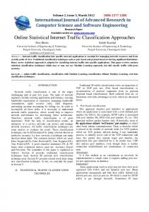
Figure 1: Summary of the procedure used to derive ~ for a certain protocol, starting the mask vector M from flows generated by such protocol.

to capture the traffic traces and with the clock resolution of the capture device, and binned accordingly. In case of Tcpdump [16] used on off-the-shelf hardware, the P DFi plane can be realistically binned along the (log10 ) ∆t-axis from 10−7 to 103 (seconds), with step 0.012 . Each resulting P DFi matrix in our example above would be 1461x1001. Finally, if L + 1 is the number of packets of the longer-lived flows used to analyze a certain protocol, we order the resulting L ~ . P DFi into the Probability Density Function vector P DF

3.2

In order to classify an unknown traffic flow given a set ~ s we need to check if the behavior of the of different P DF flow is statistically compatible with the description given by ~ s; furthermore, we need to choose at least one of the P DF ~ describes it better. which P DF We are looking for a definition of an anomaly score S that could describe “how statistically far” an unknown flow F ~ . A basic building block of is from a given protocol P DF such anomaly score is the value that the i − th component ~ of P DF assumes in Pi , with Pi being the i − th pair of the unknown flow. This value should give us the correlation between the unknown flow’s i − th packet and the applica~ used: the tion layer protocol described by the specific P DF higher the value, the higher the probability that the flow was generated by such protocol. However, the random variables that are used to build each ~ protocol’s P DF are affected by forms of “noise”, such as variability in round trip times caused by network congestion, changes in MTU values caused by alternate paths between sender and receiver, and differences in the local implementation of each protocol’s state machine. A way we devised to take into account noise effects on (s, ∆t) when calculating the anomaly score of a given packet Pi against a P DFi , is to also consider the values of P DFi in a region close to Pi . ~ as To this end, we introduce the concept of protocol mask M ~ is defined the basic component of a protocol fingerprint. M as the vector of L matrices resulting from the application ~ vector, of a Gaussian filter to each component of the P DF and rescaling every resulting matrix so that it still sums to 1, according to the properties of any PDF.

Protocol fingerprint precursors: Probability Density Function vectors

The generation of a given application layer protocol’s fingerprint starts from the evaluation of a set of L Probability Density Functions P DFi , estimated from a set of flows (a training set) generated by the same, known protocol, and captured by a monitoring device. The i − th P DFi is built on all the i−th pairs Pi belonging to those flows that are atleast i+1 packets long. The objective of P DFi is to describe the behavior of the i-th packets on the plane (packet-size s, inter-arrival time ∆t) for a certain protocol. The rationale behind using only the i−th pairs of each flow to build P DFi is to take into account not only the statistics of packet size and inter-arrival time, but also the order of each packet as seen by the classifier. Variable s is discrete and assumes values in a range dimensioned according to the minimum and maximum size of an IP packet on the network interface used to collect the traces. For example, on an Ethernet link, s would range from 40 to 1500 (bytes). Variable ∆t is, instead, sampled with resolution coherent with the speed of the network interface used

2 Note that although the binning of the ∆t axis is done to accept time-stamp differences of as little as 10−7 seconds, in our case this is a value that is far too conservative, since Tcpdump will not be able to reach this kind of accuracy on off-the-shelf hardware. However, this fact does not impact the correctness of our methodology, since the same inaccuracies imputable to Tcpdump are expected to affect homogeneously the generation of every protocol’s P DFi .

1 The extension of our work to other kinds of transport layer protocols, such as UDP, is left as future work.


Anomaly scores and protocol masks

9


1: 2: 3: 4: 5: 6: 7:

Figure 1 shows a summary of the procedure to derive the ~ for a certain protocol. The rationale behind mask vector M the idea that the filtering operation helps countering the effects of the forms of noise described above is simple, and it is best explained with an example. Let us consider a packet that would fall on the barycenter of a highly-populated part of a given protocol’s P DFi in the absence of noise, therefore contributing positively to the probability that the flow under consideration was generated by such protocol. However, because of even slight variations on RTTs, such packet might now fall outside the highly-populated part of the P DFi , possibly even on a non-populated part. Since applying a Gaussian filter to each P DFi plane smooths its values, the operation should help the classifier recover from such errors induced by noise3 . Naturally, the tuning of the parameters of the Gaussian filter will be one of the main design choice of the classifier, as we will see in the following. We can now proceed to the actual definition of anomaly ~ score S. We start by introducing an anomaly score vector A, whose i−th component Ai is a function of the value Mi (Pi ). ~ is defined as follows: The i − th component of vector A Ai (Pi , Mi ) =

1 , max (ε, Mi (Pi ))

Figure 2: Classification algorithm. this is instrumental in the classification algorithm to help it decide when an unknown flow is “far enough” from each fingerprinted protocol to be considered “not classifiable”. For this purpose we define protocol p’s anomaly score threshold T~ p as the vector composed by the sum of the mean µ and standard deviation σ of the anomaly scores of the flows used to build p’s mask vector. The T~ p vector is composed of as ~ Each element many elements as the anomaly score vector A. of T~ p can be calculated as: ” ” “ “ ~ p }, ~ p } + σ{Sn F, M (3) Tnp = µ{Sn F, M

(1)

~ p is protocol p’s mask vector and F represents where M the set of flows used to build it. The threshold vector T~ p represents the upper bound of the anomaly score that a flow can reach to be considered generated by protocol p.

where Mi (Pi ) is the value of Mi calculated in Pi , and ε is a small positive quantity. We introduce the term ε to let the score be always finite, even when Mi is zero in Pi 4 . By construction, the following will hold true for any value of Pi on the plane (s, ∆t): 1 ≤ Ai (Pi , Mi ) ≤ ε−1 . ~ Starting from the definition of anomaly score vector A ~ as we can now define the anomaly score S of F versus M follows: Pn “ ” ~ = [ i=1 Ai (Pi , Mi ) /n] − Amin , (2) Sn F, M Amax − Amin

3.4

4.

CLASSIFICATION ALGORITHM

Building on the definition of protocol fingerprint and anomaly score, we can introduce the following classification algorithm, outlined in Figure 2. In practice, given K protocol ~ j , T~ j }, with 1 ≤ j ≤ K, and an unfingerprints Φj = {M known flow F of which we have seen n packets, we start by calculating F ’s anomaly score Sn against all known protocol fingerprints (lines 1-2). This gives an indication of “how far” the flow is from each fingerprint’s protocol mask. Thresholds play a role in line 3, where the flow’s anomaly scores are normalized with respect to each fingerprint’s threshold. The protocol whose fingerprint yields the minimum of this normalized anomaly score for F is considered the one which the flow belongs to if the related anomaly score is less than or equal to its threshold (lines 4-5). Otherwise F is considered “unknown” (lines 6-7). The fact that we consider anomaly scores normalized against thresholds is key to the classification algorithm. The reason for the normalization operation is intuitive and better explained with an example. Figure 3 shows the hypothetical values of anomaly score of a given flow against the HTTP

Anomaly score thresholds

Protocol masks summarize one side of the statistical behavior of flows produced by the same protocol. Other statistical elements at the basis of our definition of protocol fingerprint are the mean and standard deviation of the anomaly scores of the flows used to build a given protocol mask: 3

Indeed, other forms of noise such as packet loss and packet reordering would also have to be considered, in this case allowing values from P DFi close to the one being considered to have an impact on the anomaly score. We will study countermeasures to these other types of noise in future works. 4 ε can be arbitrarily small. Given its purpose, i.e., to let the score be finite even when the value of Mi is zero, in this paper we assume that ε is an order of magnitude smaller than the smallest non-zero value of Mi . Values smaller than this would not affect the results presented here.


Protocol fingerprints

We define protocol p’s fingerprint Φp as the union of the two statistical vectors defined above, i.e., protocol p’s mask ~ p and protocol p’s threshold vector T~ p . The tenet vector M ~ p , T~ p } represents, in a comof this paper is that Φp = {M pact and efficient way, the main statistical properties of the flows produced by protocol p, and can therefore be used to classify flows produced by it. Note that the fingerprints are supposed to be site-dependent, i.e., they are not supposed to be transportable from one network gateway to another. Each site would have to build its own fingerprints. In general, this technique assumes that the classifier is placed on the same network segment used for the training phase.

where 1 ≤ n ≤ N , N is the minimum between the number of pairs composing F and L, and Amin,max are the allowed −1 extreme values of A as defined above, “ i.e.,” 1 and ε , re~ ≤ 1. spectively. This implies that 0 ≤ Sn F, M Sn is a function of n, the number of packets of the flow we are considering. Using this definition, it is possible to calculate the anomaly score of a given flow against a given protocol mask as the classifier “sees” the flow: as more packets arrive at the classifier, the flow’s anomaly score from a given protocol mask will be calculated including more elements from the mask vector.

3.3

for (j = 1; j ≤ K; j++): ´ ` compute Sn F, M j as in Eq.2 ` ´ Xnj = Sn F, M j /Tnj if minj {Xnj } ≤ 1: F ∈ argminj {Xnj } else: F ∈ unknown

10


an anomaly score for a flow of which we have seen n packets is as fast as the algebraic sum of n ordered terms obtained looking up values in PDF elements.

4.1.2 Figure 3: Example: use of thresholds in the classification algorithm. and POP3 protocol fingerprints, together with the respective threshold values. In the example, even though the flow’s score against HTTP is higher than its score against POP3, the former is farther than the latter, in relative terms, from the respective threshold. Therefore, it makes sense to classify the flow as HTTP rather then POP3. As we will see, experimental results support this intuition.

4.1

Using the technique in practice

The application of this technique to classify TCP flows on a real network is relatively simple, and can be summarized in the following steps: a. Collect traffic traces on the edge gateway of the network. This can involve using Tcpdump or any other traffic-capture mechanism available. These traces will serve as training set for our classification technique. b. Pre-classify the traces by means of any effective mechanism, either payload or header based, statistical or deterministic, such as Snort, Bro, the techniques proposed in [5, 13, 12], or a combination of these mechanisms. We will discuss how the accuracy of the fingerprinting phase is essential to this process later in the paper. c. Build protocol fingerprints based on the pre-classified traces following the procedures described in Section 3. Install the fingerprints on the classification engine. d. Start the classification engine built on the algorithm introduced in Section 4. This activity can be performed on live traffic.

5. 5.1

e. Periodically, if necessary, update the fingerprints by running steps a through c again.

Applicability of the classification algorithm

The way the algorithm is devised allows its application to the dynamic classification of flows: as the classifier sees more packets of each flow, it can increase the chances of correctly classifying it. The way the performance of our algorithm is linked in practice to the number of packets analyzed for each flow will be discussed in the following of this paper. The scenario we imagine for practical uses of our algorithm should lead to a low computational load at the classifier: in fact, network administrators are usually interested in actively managing only a fraction of the protocols running on their networks; hence only a few fingerprints should be stored and examined to prioritize a limited number of critical services or block others. Indeed the calculation of


EXPERIMENTAL ANALYSIS Testbed setup, traffic traces and protocol fingerprints

We tested the validity of the classification technique with traffic traces collected at the edge gateway of our faculty’s campus network. This networking infrastructure, which consists of around one thousand workstations equipped with a variety of operating systems, is composed of several 1000BaseTX layer-2 segments routed through a Linux-based dualprocessor box. Connectivity is provided to end users by either 100BaseT links or 802.11b/g Access Points. All the experiments described in this section were run on the 24Mb/s link that connects the edge router to the Internet. We ran the experimental analysis by following pretty closely what a network administrator would have to do to implement our classification technique. At first we analyzed the traffic aggregate in order to determine how the bandwidth to the Internet is shared among the most used application protocols. We discovered that on average more than 60% of the available bandwidth of our link to the Internet on any given working day is occupied by flows whose source or des-

A few notes on the applicability of this technique are in order.

4.1.1

Building accurate protocol fingerprints

The accuracy of the tools used in step b is critical. Preclassification of the flows that will be used to build fingerprints should introduce as little noise as possible: for example, when building HTTP fingerprints, the inclusion of HTTP flows tunneling peer-to-peer bulk data should be avoided. However, the validation of training sets is widely recognized as a very hard problem [5]. A combination of different payload-based classifiers could, in many cases, help: even though computationally inefficient, this combination of mechanisms would have to be seldom run, i.e., when the fingerprints have to be created for the first time and when they have to be updated as application layer protocols evolve. In the preliminary experimental analysis reported in this paper we use a simple technique: we derive our training sets by applying a payload-based pattern-matching technique to all traffic to select flows that were generated by each protocol we need to fingerprint. This approach has two drawbacks. Firstly, this mechanism is as precise as the pattern-matching technique is. In the case of a relatively controlled environment and with a reduced set of protocols such as the one considered in the experimental analysis described in the following, the precision of the pattern-matching technique is enough to produce accurate fingerprints. Secondly, this technique can be inefficient in the sense that only a fraction of all traffic to, say, port 110 is pre-classified successfully: this leads to the need for more data than theoretically needed to train the system. In general, the results presented in this paper are based on the assumption that accurate fingerprints are available, which, as said before, is a hard research problem to solve. While a simple technique such as one based on pattern-matching can be enough in specific cases like the one considered in this paper, a more robust and generic approach at constructing accurate fingerprints will have to be investigated in the future.

11


tination TCP port is either 80 (registered for HTTP), 110 (POP3) or 25 (SMTP). Therefore, we started by collecting a training set for the purpose of fingerprinting these three protocols: to this end we used Tcpdump for one week – daytime-only5 – to capture flows matching the HTTP, POP3 or SMTP standard ports. The resulting 40+ GB traces were then run through a payload-based, pattern-matching classifier that we built, according to the patterns described in [5] and [17]. Among the flows that passed the pattern-matching step twenty thousand were randomly selected to generate HTTP, POP3 and SMTP fingerprints by following the procedure outlined in Section 3. In other words, flows that entered the training set were randomly chosen, after the pre-classification phase, to be uniformly distributed among all the flows collected during the training week. After a couple of weeks, we collected another week worth of traffic, daytime-only, to create the evaluation set which we then used to assess the validity of the classification algorithm. Here we also randomly selected the evaluation set so that flows used to build it were uniformly distributed along all week. In order to certify the application layer protocols that generated the evaluation set, we manually inspected the payloads of the selected flows6 . This activity put each flow in one of four subsets of the evaluation set: one for HTTP, one for POP3, one for SMTP, and one for flows not belonging to any of the above classes, which we named OTHER. Besides OTHER, which was built with five thousand flows, every evaluation subset ended up being composed of ten thousand flows. The knowledge of the application layer protocol that generated each flow in the evaluation set is at the basis of the performance analysis of the classification engine against the parameters defined in the following section.

5.2

Starting from these quantities, we can define the following two performance parameters. The hit ratio Hr of our classification engine for a given protocol p is defined as in expression 4(a): eˆp eˇp (a), F+ = p (b). (4) p E e Hr measures the percentage of flows from the evaluation subset p that were correctly classified. This gives an indication of how good the classifier is at using p’s fingerprint to characterize p’s behavior. Note that Hr is calculated over E p rather than over ep because the hit ratio should express how many of the actual flows of a given protocol (therefore E p ) were correctly classified. Defining Hr over ep could be misleading. For example, if E p were 100, ep were 10 and eˇp were 10, only looking at the last two figures one might assume the classifier was perfect, while it was in fact classifying correctly only 10% of the traffic. The hit-ratio alone is clearly not enough to describe the validity of the algorithm. A network manager would be interested in knowing how many of the flows classified as protocol p were actually belonging to a subset that was not p. To evaluate this performance criteria we introduce a falsepositive ratio parameter F+ , defined as in expression 4(b). The false-positive ratio expresses, in some sense, the trustworthiness of the classifier: in other words, this parameter answers the question “out of x number of flows classified as protocol p, what’s the fraction that was not really produced by p?” Hr =

5.3

In Table 1 we present the hit ratio and the false-positive ratio of the classification engine described in Sections 3 and 4 for all the four categories of traffic. The classifier performs reasonably well, showing hit-ratios well above 90% for each of the protocols considered and the false positive ratios around 6% in the worst case.

Performance parameters

By running each flow of the evaluation set through our classifier we can expect four types of answer: either the classifier thinks the flow is HTTP, POP3, SMTP, or “none of the above”, i.e., OTHER. Clearly, the classifier can be mistaken, and we need to define performance parameters to evaluate different types of errors. The following quantities are the basis for such parameters. For p varying in [POP3,HTTP,SMTP,OTHER] we define:

Protocol HTTP SMTP POP3 Other

• E p as the number of flows of protocol p in the evaluation set, as certified by the pattern-matching/by-hand pre-classification procedure. For example, with the data presented in the previous section, the following would hold: E HT T P = E P OP 3 = E SM T P = 10000.

Hr 91.76% 94.51% 94.58% 90.64%

F+ 6.38% 3.06% 3.08% N.A.

Table 1: Hit ratios and false positive ratios (optimal parameters). These results were obtained by tuning the classifier’s configuration parameters with what seems to be the optimum for the traffic traces we have considered. In particular, each fingerprint was built with twenty thousands flows from the training set, using a 45x45 window size for the Gaussian filter (see Section 3.2). Each fingerprint’s threshold (see Section 3.3) was calculated as a simple sum of the standard deviation and mean values of the anomaly scores. We used Fclient fingerprints, because we found out that they gave better results than Fserver ones (we will discuss this aspect in detail in Section 6). Finally, the classifier was instructed to take its decision after evaluating the 4th Fclient packet. This is the most important configuration parameter of all, because it impacts the ability of the classifier to work almost in real time, i.e., as it sees the first packets of each flow.

• ep as the total number of flows from the evaluation set classified as protocol p by our classifier. • eˇp as the number of flows correctly classified as protocol p. By definition, eˇp ≤ E p and eˇp ≤ ep . • eˆp as the number of flows incorrectly classified as protocol p. 5 The amount of outgoing traffic generated during the night by the three analyzed protocols was negligible compared to what generated during working hours. 6 Although this was a rather tedious operation, Manuel and Maurizio knew that it was a necessary precondition to the correctness of the results. The other authors thank them for spending quite some time performing it.


Numerical results: optimal parameters

12


Figure 5: Fraction of flows in the training sets with a least n packets. that the wider the threshold for a given protocol, the higher the hit ratio will be for that protocol. On the other hand, increasing the threshold should also increase the false-positive ratio, therefore one should try to find an optimal value for this parameter, so that both the false-positive and hit ratio are optimized.

Figure 4: Hit ratio and false-positive ratio versus packet number where the classifier took its decision.

5.4

Sensitivity to configuration parameters

In this section we explore what influence the configuration parameters of the classifier have on its performance, as defined in Section 5.2, starting with the optimal values described above.

5.4.1

Sensitivity to the packet number

Figure 4 shows the classification results as a function of the packet number n where the classifier takes its decision. For the Fclient flows we are considering, n = 3 is the first packet sent by the client after the three-way-handshake, and thus it is the first one that could be used for a meaningful statistical classification. The figure shows that the combination of hit ratio and false-positive ratio reaches an optimum on a given packet number n after which the performance of the classifier decreases, and that n is different for different protocols. It seems that the classifier should decide whether a flow is HTTP at the 3rd Fclient packet, but should wait the 4th packet to make the decision for SMTP, and the 4th or 5th packet for POP3. Even if this behavior can seem counterintuitive at first, it can be explained by looking at the way the training set for each protocol was built. Figure 5 shows, for the training set of each protocol, the fraction of flows that have at least n packets. While almost all of the twenty thousand flows used to build the SMTP fingerprint have at least five packets, only around 50 to 60% of the ones used to build the HTTP fingerprint are 5-packets long. There is a clear correspondence between the packet number where the performance of the algorithm peaks and the packet n where the number of flows in the training set at least n-packets long starts decreasing. In summary, as it could be expected, the number of flows used to build a protocol fingerprint is correlated to the performance of the algorithm. We will see more about this topic later in this section.

5.4.2

Figure 6: Hit ratio and false-positive ratio versus threshold’s width parameter x. We have studied how the performance of the algorithm changes as the definition of threshold changes as well. First, let us redefine each component of the anomaly score threshold by adding a multiplier to the second term of Equation 3 as follows: “ ” “ ” ~ p } + x · σ{Sn F, M ~ p }. (5) Tnp = µ{Sn F, M Figure 6 shows that the optimal value for x, i.e., the value that yields the best compromise between hit and falsepositive ratios is “1”. In other words, with the types of protocols analyzed in this paper, a small threshold value seems to be appropriate for obtaining the best compromise between hit ratios and false positive ratios. We expect this

Sensitivity to threshold’s parameters

The threshold vector is an integral part of the definition of protocol fingerprints (see Section 3.3). It can be expected


13


to change when we will analyze the performance of this technique applied to other protocols, more similar to one another than the ones considered in these experiments.

5.4.3

Sensitivity to the window size of the Gaussian filter

The window size of the Gaussian filter used to build protocol fingerprints (see Section 3) affects the precision with which the classifier compares a flow with the statistical characteristics of a protocol’s training set. The larger the window size, the higher the possibility of the classifier to “spot” a certain protocol p flow, and therefore the higher the hit ratio for that protocol. However, higher values for the window size also increase the false-positive ratio, similarly to what happens for the anomaly score threshold. Since changes to the window size affect differently the behavior of the classifier with different protocols, we define its optimal value as the one that minimizes the following expression: ! K “ ” X i i , (6) minx,y 1 − Hr + F +

Figure 7: Hit ratio and false-positive ratio versus size of training sets (in number of flows).

i=1

where K is the number of protocols of the evaluation set and (x, y) represent the window size of the Gaussian filter. The sum in Equation 6 takes into account the distance between the hit-ratio of a set of given protocols and the maximum hit-ratio (100%) and the false positive ratio of each protocol. During our experiments, we tested different values for (x, y): starting from a conservative, and minimum valid value of (3,3) and going up to (45,45), hit ratios went from 11.77% to 91.76% for HTTP, from 86.49% to 94.51% for SMTP and from 68.11% to 94.58% for POP3, while falsepositive ratios increased from very close to 0% to around 3% for SMTP and POP3, although they did not change significantly for HTTP. This supports the intuition that a ~ helps countering the smoothing filter applied on the P DF noisy factors described in Section 3.2. We probably have not found the optimum yet, since the best results were obtained with the Gaussian filter set at the maximum value we analyzed. We will continue analyzing this parameter in the future7 .

5.4.4

that even though the patterns available today are pretty good at spotting HTTP traffic, the statistical classifier performs better for both SMTP and POP3 flows in our scenario. On the other hand however, the pattern-matching pre-classifier presents virtually no false-positives, which, again in our scenario, allowed its use as a pre-classification device for the generation of accurate protocol fingerprints. Accuracy of training sets: an open problem. The pre-classification of the flows that are used to build fingerprints is still an open issue: as an example, at this stage of development, the pattern-matching pre-classifier that we built, based on [5] and [17], drops more than 20% of any given set of POP3 flows. Even more problematic is the fact that pre-classifying other types of traffic such as peer-to-peer would be much more difficult, even with advanced forms of pattern-matching techniques. Note that without a fingerprint our technique is completely ineffective: at this time we do not know if a fingerprint derived at site X could be made usable at site Y. Both of these problems, i.e., the “transportability” of fingerprints, and the availability and accuracy of pre-classification techniques will be the subject of future work. A few notes on the complexity of the technique. Aside from the issue of fingerprinting, the way the classification algorithm works indicates that the engine could be straightforwardly implemented in hardware based on any of the current integrated-circuit technologies. Such device should only have as much memory as needed to record the desired number of fingerprints a network administrator would need, and the computation of the anomaly score of a flow

Sensitivity to the size of the training sets

Figure 7 shows Hr as a function of the number of Fclient flows used to build protocol fingerprints: while POP3 and SMTP are well characterized with just a thousand flows, HTTP requires a larger training set to be correctly classified. False-positive ratios seem to be less dependent on the size of the training sets. At any rate, the total number of flows per protocol required to effectively train the system is perfectly reasonable: a few days of network traces can be enough to create fingerprints for the protocols we have considered.

6.

DISCUSSION Protocol HTTP SMTP POP3 Other

A rough comparison with a payload-based classifier. Table 2 shows the classification results of the patternmatching pre-classifier applied to the same evaluation set we described in the previous section. These results highlight 7 The analysis of how the performance of the algorithm is affected by the parameters of the Gaussian filter is very computationally intensive. With the time and computing resources at hand we were able to test the parameters in the limited range described above.


Hr 99.10% 85.94% 79.67% 99+%

P kt.# 3/4 (Fserver ) 2/3 (Fserver ) 2 (Fserver ) N.A.

Table 2: Hit ratios and packet where the match occurred for the pattern-matching pre-classifier.

14


should be as simple as an adder. In fact, the classification operation can be as simple as the algebraic sum of n values obtained from an ordered set of PDFs, multiplied by the number of fingerprinted protocols. Using Fclient and Fserver data, and where the classifier should be placed. As we have seen, in the scenario we considered the technique performs better when applied to Fclient flows than to Fserver ones: in general, we found that hit ratios when using Fserver flows were from 10 to 30% lower than the ones obtained using Fclient ones. This can be justified by the fact that the characteristics of the parameters we are observing are more deterministic for Fclient than for Fserver flows, since the classifier is closer to clients than to servers. This affects in particular the statistics of the ∆t parameter. We see at least two issues in this respect that will require further analysis in the future: an issue of applicability of the technique to environments where the classifier is not close to clients nor to servers, and an issue of combining Fclient and Fserver data in the classification algorithm. As to the first issue, the experimental analysis described in this paper was performed on network traces captured at the edge router of our faculty’s network. Our choice is perfectly suited to a modern network scenario where the actions of packet classification and marking are delegated to edge gateways. In case this technique should be applied to core networks, this assumption would not hold. However, the preliminary results we obtained using Fserver data, although not conclusive, indicate that the performance of the algorithm should decline gracefully when moving the classifier away from the edge of the network. Clearly, and this is related to the second issue, a better classification algorithm should take into account both Fclient and Fserver data. We have tried simple combinations of the Anomaly Score series obtained from the two data directions (e.g., linear combination, quadratic sums, etc.), but none of these simple combination techniques fare better than looking at only one direction of the flow. Without doubt there is much space for improvement in this area. On the precision of the measuring devices. The fingerprinting device and the classifying device are the same in our experiments. We know pcap is not precise, but even with its current level of precision on standard hardware it seems to be able to cope with the requirements of the classification algorithm we are proposing, at least in our environment. In networks with higher-speed interfaces it will be necessary that both the fingerprinting device and the classifier have dedicated hardware for precise network measurements. We will analyze the impact of the imprecision introduced by the measuring device on the performance of the classifier in future works.

7.

thermore, in this paper we have considered HTTP as a homogeneous application protocol: it would be interesting to analyze whether the classification algorithm can be tuned to discriminate among the different application types HTTP can be used for, such as images, text, etc. By means of the Gaussian filtering operation on PDFs we have introduced what seems to be an effective way for the classifier to take into account some of the noisy factors that affect RTTs and packet size. Clearly, these are not the only noise factors that a classifier should take into account. What remains to be investigated is how packet loss and packet reordering affect the performance of this classifier, and how to best cope with them. One approach could be to consider consecutive elements of the PDF vector when evaluating the contribution of a given packet to the Anomaly Score. Furthermore, the way the algorithm responds to attacks against the classification engine, such as deliberate packet reordering or active modification of packet jitter and packet size, needs to be investigated. In this paper we have assumed that protocol fingerprints are site-dependent and must be seldom updated. In future works we plan to mitigate (or validate) these assumptions collecting the data from different networks in different time intervals and therefore, obtaining several training sets. We will then analyze the differences between the fingerprints of the same protocol built with different training sets, and explore the possibility, if any, to modify one site’s fingerprints to adapt them to the use on a different site. The protocol fingerprints derived during our preliminary experimental analysis were built with a training set that is fully reliable. However, the validation of training sets is widely recognized as a hard research problem: the ability to generate accurate fingerprints could become one of the major showstopper to any trained statistical approach to traffic classification. In view of this problem, we plan to start analyzing how the accuracy of the classifier is affected by fingerprints that are not 100% precise, i.e., that have been derived by a set of traffic flows that contains both the protocol under consideration and other protocols. The way the classifier responds to inaccurate fingerprints will give us an indication of how precise the pre-classification phase will have to be for our technique to behave acceptably. By examination of the classification algorithm, it is simple to derive that its computational complexity is as low as the algebraic sum of a few terms obtained by looking up values in PDF tables, multiplied by the number of fingerprints under consideration. Further, more rigorous analysis will be required to ascertain the other aspects related to the (supposedly low) complexity of the algorithm, both in terms of its memory occupation, its amenability to hardware-assisted implementation, and the computational costs of the training phase. Finally, the simple, preliminary definitions of protocol fingerprint and classification algorithm presented in this paper offer significant other directions of improvement, including for example the use of second-order statistical parameters, combining the Fclient and Fserver metrics and assigning different weights to each component of the protocol mask vectors.

FUTURE WORK

The experimental environment described in this paper allowed us to analyze the performance of this classification technique on a reduced set of protocols. Furthermore, such protocols are in some ways “easy” to classify, since their characteristics are different enough so that a statistical classifier might have an easy job in picking up their specific behavior. The biggest contribution to the analysis of the general applicability of this technique will come from its application to a larger data set, in particular one that comprises what constitutes a very significant portion of traffic on the Internet, i.e., Voice over IP and Peer-to-Peer. Fur-


8.

CONCLUSIONS

In this paper we have proposed a statistical classification technique based on the analysis of simple properties of network traffic. We introduced what we call protocol finger-

15


prints, i.e., quantities that are at the basis of the training phase, and that express, in a compact and efficient way, the main statistical properties used to characterize each protocol: inter-arrival times, size of the IP packets, and the order in which they are seen by the classifier. Preliminary experimental analysis has shown promising results: the technique can determine with a relatively small error ratio the application protocol behind network flows, at least with a reduced set of protocols, when the classifier has been properly trained. The analysis has also shown that the Gaussian filtering operation used to derive protocol fingerprints seems instrumental in the ability of the classifier to deal with noise such as jitter and unexpected changes in packet size. Furthermore, the normalized thresholds used by the classification algorithm can be an effective tool in discriminating when traffic does not belong to any of the fingerprinted categories: this improves the effectiveness of the technique in dealing with non-fingerprinted traffic, which in turn is fundamental given the well known problems related to the accuracy, or lack of thereof, of generally-applicable training mechanisms. Our algorithm and definition of fingerprint are still at an early stage of development: the magnitude of work needed to prove its general applicability and the issues that still need to be analyzed have been discussed in Sections 6 and 7. However, we believe that the preliminary results presented in this paper are promising enough to warrant further work on this technique.

9.

[9] F. Hern´ andez-Campos, F. Donelson Smith, K. Jeffay, and A. B. Nobel. Statistical Clustering of Internet Communications Patterns. In Computing Science and Statistics, volume 35, July 2003. [10] A. McGregor, M. Hall, P. Lorier, and J. Brunskill. Flow Clustering Using Machine Learning Techniques. In Proceedings of the 5th Passive and Active Measurement Workshop (PAM 2004), pages 205–214, Antibes Juan-les-Pins, France, March 2004. [11] M. Roughan, S. Sen, O. Spatscheck, and N. Duffield. Class-of-service mapping for QoS: a statistical signature-based approach to IP traffic classification. In IMC ’04: Proceedings of the 4th ACM SIGCOMM conference on Internet measurement, pages 135–148, Taormina, Sicily, Italy, October 2004. [12] A. W. Moore and D. Zuev. Internet traffic classification using bayesian analysis techniques. In SIGMETRICS ’05: Proceedings of the 2005 ACM SIGMETRICS International Conference on Measurement and Modeling of Computer Systems, pages 50–60, Banff, Alberta, Canada, June 2005. [13] A. W. Moore and K. Papagiannaki. Toward the Accurate Identification of Network Applications. In Proceedings of the 6th Passive and Active Measurement Workshop (PAM 2005), pages 41–54, October 2005. [14] L. Bernaille, R. Teixeira, and K. Salamatian. Early Application Identification. In The 2nd ADETTI/ISCTE CoNEXT Conference, Lisboa, Portugal, December 2006. [15] C. Trivedi, H. J. Trussel, A. Nilsson, and M-Y. Chow. Implicit Traffic Classification for Service Differentiation. Technical report, ITC Specialist Seminar, Wurzburg, Germany, July 2002. [16] Tcpdump/Libpcap. http://www.tcpdump.org. [17] L7 Filter. http://l7-filter.sourceforge.net.

REFERENCES

[1] D. Moore, K. Keys, R. Koga, E. Lagache, and K. C. Claffy. The CoralReef Software Suite as a Tool for System and Network Administrators. In LISA ’01: Proceedings of the 15th USENIX conference on Systems Administration, pages 133–144, San Diego, CA, USA, December 2001. [2] V. Paxson. Bro: a system for detecting network intruders in real-time. Computer Networks, 31(23–24):2435–2463, 1999. [3] M. Roesch. SNORT: Lightweight Intrusion Detection for Networks. In LISA ’99: Proceedings of the 13th USENIX Conference on Systems Administration, pages 229–238, Seattle, WA, USA, November 1999. [4] C. Dewes, A. Wichmann, and A. Feldmann. An analysis of Internet chat systems. In IMC ’03: Proceedings of the 3rd ACM SIGCOMM conference on Internet measurement, pages 51–64, Miami Beach, FL, USA, October 2003. [5] T. Karagiannis, K. Papagiannaki, and M. Faloutsos. BLINC: multilevel traffic classification in the dark. In SIGCOMM’05: Proceedings of the 2005 conference on Applications, technologies, architectures, and protocols for computer communications, pages 229–240, Philadelphia, PA, USA, August 2005. [6] V. Paxson. Empirically derived analytic models of wide-area TCP connections. IEEE/ACM Trans. Netw., 2(4):316–336, 1994. [7] V. Paxson and S. Floyd. Wide area traffic: the failure of Poisson modeling. IEEE/ACM Trans. Netw., 3(3):226–244, 1995. [8] A. Mena and J. Heidemann. An Empirical Study of Real Audio Traffic. In Proceedings of the IEEE Infocom, pages 101–110, Tel-Aviv, Israel, March 2000.


APPENDIX A. PUBLICLY AVAILABLE TRACES AND TRAFFIC CLASSIFICATION We have been asked why we are not using publicly-available packet traces to validate our classification technique. In fact, several organizations routinely release anonymized packet traces from backbone networks. Two of them are CAIDA and NLANR. The problem with these traces is that they do not contain, for understandable privacy and security reasons, any useful information at the application level, making their use impractical (or even impossible) for research in traffic classification. It would be useful if researchers in this area would start sharing anonymized packet traces with full classification meta-data. Before anonymizing traces these organizations could classify each flow, and add such classification information as meta-data to the released traces. As soon as we obtain the necessary clearance, we intend to release anonymized versions of the traces used to produce this work, together with full meta-data classification information. This will provide other researchers with the possibility of testing other algorithms on the same data we used and, hopefully, will serve as a first, small incentive to other larger organizations to do the same.

16
