Apr 4, 1988 - segments, (iii) statistical analysis of all distance subclasses and assessment of the accumulated "noise" that may blur the basic topology of ...
Proc. Natl. Acad. Sci. USA Vol. 85, pp. 5913-5917, August 1988 Biophysics
Statistical geometry in sequence space: A method of quantitative comparative sequence analysis (nucleic acids/topology of divergence/Hamming metric/evolutionary noise)
MANFRED EIGEN*, RUTHILD WINKLER-OSWATITSCH*, AND ANDREAS DRESSt *Max-Planck-Institut fur Biophysikalische Chemie, D 3400 Gottingen, Federal Republic of Germany; and tFakultat fur Mathematik, Universitat Bielefeld, D 4800 Bielefeld, Federal Republic of Germany
Contributed by Manfred Eigen, April 4, 1988
substitution probabilities are uniform and time invariant at all positions. Neither assumption is realistic. Nucleotide substitution at a particular position depends (i) on the mutation rate of that particular nucleotide and (ii) on the probability of selective fixation of the mutation after it has occurred. Transitions-i.e., changes within a base class of R (purines) or Y (pyrimidines)-are usually found more frequently than transversions-i.e., changes that alter the base class. Kimura (1) has devised an equation that takes different rates into account; it has been generalized (2) to apply to any possible kind of substitution. However, this kind of mutational specificity is a small part of the metric nonuniformities usually encountered. Variability may range from total invariance at some positions to hypervariability at others. It is predominantly related to the acceptance of mutations, which depends on functional constraints in a subtle manner. To demonstrate the consequences of metric nonuniformities, let us consider parallel divergence. A set of n sequences based on four different symbols is assumed to have separated from a common precursor at zero time and subsequently evolved in parallel. Time is related to a mutation distance A that measures all accepted mutations (including parallel and reverse) in a sequence comprising v positions. Supposing uniform substitution rates, we have three separation distances (3): (i) the average distance of individual pairs i and k,
A statistical method of comparative sequence ABSTRACT analysis that combines horizontal and vertical correlations among aligned sequences is introduced. It is based on the analysis mainly of quartet combinations of sequences considered as geometric configurations in sequence space. Numerical invariants related to relative internal segment lengths are assigned to each such configuration and statistical averages of these invariants are established. They are used for internal calibration of the topology of divergence and for quantitative determination of the noise level. Comparison of computer simulations with experimental data reveals the high sensitivity of assignment of basic topologies even if much randomized. In addition, these procedures are checked by vertical analysis of the aligned sequences to allow the study of divergences with positionally varying substitution probabilities.
Introduction
Sequence analysis of nucleic acids has become routine. As data accumulate at an ever increasing rate, we are witnessing the origin and growth of a new kind of library: A data bank accessible by a worldwide computer network to provide the sequence of any archived gene. In this situation, it is important to have reliable methods for comparative sequence analyses that uncover the kinship relationships hidden in sets of sequences. We introduce here a concept of comparative sequence analysis of nucleic acids that we call statistical geometry. It is particularly useful for the analysis of "old" relationships that have randomized to a large extent. It provides (i) a test for the uniformity of distance assignment through positional checking of substitution probabilities, (ii) reliable assignment of the topology of divergence by partitioning distances into segments according to vertical coincidences in an alignment and the construction of geometries that correlate these segments, (iii) statistical analysis of all distance subclasses and assessment of the accumulated "noise" that may blur the basic topology of divergence, and (iv) an estimate of the relative temporal order of divergence based on both the basic topology and its superimposed noise.
dik
= 3v/4{1 - exp(-8A/3v)};
[1]
(ii) the average distance of individuals from the precursor at A/v = 0 (i.e., zero time)
dio = 3v/4{1
-
exp(-4A/3v)};
[2]
(iii) the distance between the master (m) or consensus sequence and the precursor
dmo
=
v/2 erfc{[
{11
+ 3
n/6
exp(-4A/3v)} {1 [3
x
Row and Column Statistics of Aligned Sequences
-
exp( - 4A/3v)}
exp(-4A/3v)
-
1/2
(3/2n)1/2},
[3]
where erfc {x} means complementary error function:
For any pair of aligned sequences the (Hamming) distance is defined as the number of positions that are occupied by different nucleotides. In this way, for any set of n aligned sequences, the associated system of distances induces the structure of a metric space defined on this set. In comparative sequence analysis, distance is considered to be a measure of temporal evolutionary separation, tacitly supposing that
2 r1/2
J exp( - t2)dt. X
The master or consensus sequence has the nucleotide that appears most often at each position. Fig. 1 shows computersimulated curves for d;,, d3,, and dmO as functions of A/lv for n = 30 sequences of length v = 30. What is surprising about these curves is how well the master sequence resembles the initial sequence even when
The publication costs of this article were defrayed in part by page charge
payment. This article must therefore be hereby marked "advertisement" in accordance with 18 U.S.C. §1734 solely to indicate this fact. 5913
Biophysics: Eigen et al.
5914
Proc. Natl. Acad. Sci. USA 85 (1988) _ 20-
A (v->I)
2
a)
'9
a
Ce
0
01
I
0
0
cD
Is 0
10-
0
} a)
co
a)
a)
FIG. 1. Average pair distance dik, average distance of individual from initial sequence dK and distance between initial and master sequence d,,,0 as functions of relative mutational distance A/v. Curves represent computer simulations for n = 30 and v = 30 and follow undistinguishably the analytic expressions. A, Experimental values of tRNA families (reduced to sets of 30 sequences, each composed of 30 independently variable positions). The three lower triangles give the spread of experimental distances of three master sequences (deviations from average), indicating finite d,,,o values and thereby contradicting the model of positionally uniform divergence.
the pair distances are near the limit of complete randomization. As long as dMO = 0, we may therefore replace the unknown do by the (detectable) dim-i.e., the average distance between individual and master sequences. Hence, we have two measurable parameters dik and dim that allow us to calibrate a A/v value for parallel divergence. Now we consider two extreme types of nonuniformity of substitution. First, suppose that A of the v positions in all n sequences appear to be totally invariant (beyond the tail of the Gaussian distribution that gives the fraction of positions that by chance have not changed). The curves, according to Eqs. 1 and 2 and dio - di,, would now level off at 3 =
(v4
A)
n/
* 0
-0* 00 0. 0 2 4 6 8101214161820 .000 @.
Vertical Deviations from Master
Mutation Steps (A/v)
3 -v 4
21.. I** *.0
,d
=
2dim
dik'
[4]
Second, let us assume p hypervariable positions that are entirely randomized. Now dino cannot be zero; we rather would expect a dno value of 3/4p. The distance d0o itself is not measurable. However, if dino were equal to zero, then master sequences taken from related families of sequences should turn out to be identical. The experimental values presented in Fig. 1 indicate that both invariant and hypervariable positions are present in tRNA families-possibly in addition to several degrees of "normal" variability-and that at least unweighted Hamming distances therefore do not reveal the true divergence. Is there a way to check for metric (non)uniformity? Distances result from adding up the differences between two sequences. This gives a number and irretrievably loses all positional information. To make use of positional information we have to analyze the alignment vertically rather than horizontally. In vertical analysis (3, 4), the abscissa gives the number of nucleotides in a column that are not identical with the consensus nucleotide and the ordinate gives the number of positionsft8) in the alignment corresponding to the abscissa value (8). The simulation starts at A/v = 0, where all n sequences are still identical. We have simulated parallel divergence by using uniform substitution probabilities and we recorded the obtained vertical distributions at different instances A/v. The initial singular peak quickly turns into a Gaussian that travels along the abscissa until-for large A/v values (here, A/v = 1)-it reaches a limiting position near Y2n, valid for RY sequences, or 3/4n for AUGC sequences. (Tree-like divergences do not yield simple Gaussians and depend on tree shapes.) Fig. 2 illustrates the distribution obtained for 40 tRNAs from Halobacterium volcanii. The result, typical for all tRNA
[61
FIG. 2. Column divergence statistics of a family of 40 tRNA (R, Y) of H. volcanji (5). The distribution f(S) refers to the present state of divergence S. It does not resemble a Gaussian form, as would be expected for uniform substitution probabilities. The peak at abscissa value zero indicates a large fraction of constant positions. The 30 variable positions in these sequences show all degrees of variance up to complete randomization. sequences
families (with parallel divergence), is self-explanatory: There is no uniform metric! However, from the diagram we are at least able to identify invariant, normally variable, or hypervariable positions. Having demonstrated the limitations of distance space analysis, we now ask for an approach that takes into account both horizontal and vertical kinship relationships.
Sequence Space and Distance Metric The concept of sequence space was introduced in coding theory by Hamming (6). Maynard-Smith (7) and Rechenberg (8) proposed its application to proteins and nucleic acids. The idea is implicitly involved in the quasi-species model developed by one of the authors (9) in cooperation with Schuster (10) and has been treated explicity in connection with problems of value landscapes (11-13). We begin with binary sequences, where sequence space, of dimension v, locates points attributed to each one of the 2' possible sequences of length v in such a way that all kinship neighborhoods are correctly represented. In Fig. 3 the concept is developed iteratively for dimensions one to four. If iteration is repeated v-fold, the final diagram would show a hypercube of dimension v having 2V sequences located on its corners and v2'I-' edges connecting nearest neighbors.A A neighborhood may also include points that can be reached directly by a k-error mutation jump. In nucleic acids, easily realizable values for k may range from 3 to 10 depending on population size and sequence length. The features of sequence space that distinguish it from geometric spaces amenable to our apprehension and that prove to be important for understanding the nature ofevolution are (i) the enormous "volume" encompassing 2" discrete points, (ii) the tremendous connectivity providing direct access from any point to Jk 1 (K) neighboring points of distance ok, and (iii) the shortness of detour-free paths between any two points in the hypercube. Their length never exceeds the dimension v. If four symbol classes (i.e., four nucleotides) are considered, the dimensionality increases to 2v accounting for 4" = 22v possible sequences of length v. A sequence is identified by two successive binary decisions: (i) assignment of the base classes R and Y to each position, requiring a v-dimensional hypercube; and (ii) assignment of the specific base, requiring for each point in the first hypercube a subspace that again is a hypercube of dimension Application of the sequence =
v.
*Note that the Hamming distance on the hypercube {0,1}" c R' of {0,1} sequences coincides not with the Euclidean metric in R' but with the "city block metric," which measures distances as every one would do in Manhattan according to the number of blocks one has to cross to get from A to B.
Biophysics: Eigen et al. I Z
0
00
Proc. Natl. Acad. Sci. USA 85 (1988) 10
ol
o
0
000
5915
FIG. 3. The iterative buildup of sequence space, starting with one position. Each additional position requires a doubling of the former diagram and to connect corresponding points in both diagrams (which represent nearest neighbors). The final hypercube of dimension v contains as subspaces ( )2,k hypercubes of dimension k.
space concept to evolution requires the introduction of a value topography. Value landscapes have rugged fractal structures, causing populations to accumulate on ridges and peaks in the mountainous regions (12, 13), which is the deeper reason for the metric nonuniformity commonly found in comparative sequence analysis. Statistical Geometry
Statistical geometry as such can be exemplified with mere distance relationships. Two sequences define one distance; three can always be fitted into a tripod diagram, because they yield three explicit equations for the three unknown segments. The tripod, however, may be unrealistic, because the precursor, the tripodal node, may not have existed. The truth then emerges by adding a fourth sequence. Four sequences define six distances and hence match a diagram that, in general, has six segments, as shown in Fig. 4a. The three types of segments can be obtained from AB + CD = a + b + c + d + 2x = S (small)
AC + BD = a + b + c + d + 2y = M (medium) AD + BC = a + b + c + d + 2x + 2y = L (large),
as 2x = L - M, 2y = L - S, and a + b + c + d = S + M - L. The diagram reduces to an ideal bundle if both x and y are zero and to a tree-like dendrogram, with finite branching distance y, if only x is zero. The general "net" form in Fig. 4a is due to the presence of reverse and parallel mutations,
with x being a measure of deviation from tree-likeness. (Likewise, x and y together measure the deviation from ideal bundle-likeness.) For partly randomized bundles, x and y are nonzero and of similar magnitude, with x (by definition) being the smaller of both parameters. Why do we call this method statistical geometry? There are (4) different quartets that can be formed from a set of n sequences (e.g., 27,405 for n = 30 sequences). Hence, the averages of x, y, and ¼14(a + b + c + d) for a set of n sequences usually are statistically well-defined parameters. If a tree is constructed by compromises that yield an optimal fit, and x/y average values of -0.5 or higher are found, one should be suspicious. Randomization then has proceeded so far that a tree cannot be discriminated from a bundle. On the other hand, one can prove mathematically (ref. 14; see also ref. 15 and references therein) that, if in a set of more than four sequences all x values are zero while 9 is nonzero, the total set has an exact tree-like topology. Unfortunately, statistical geometry based on distance only is not very sensitive in differentiating topologies, the main shortcoming being neglect of positional information. As explained above, such information is available from order relationships in sequence space. In sequence space formally the procedure is analogous to that in distance space: For each quartet of sequences, we analyze the optimal network connecting the four sequences in sequence space and try to reconstruct a geometry that is representative for the whole family of sequences. We begin with the case of binary (R, Y) sequences (Fig. 4b). There are eight distinguishable classes of positions in three categories: 0, all four sequences having equal occupation; 1, one sequence differing from the three others (a, f3, 'y, 8); and 2, two
A
3d
By
¼
B
FIG. 4. Representative geometries of quartet combinations of sequences in distance space (a), RY sequence space (b), and AUGC sequence space (c).
5916
~ 37
Biophysics: Eigen et al.
Proc. Natl. Acad. Sci. USA 85 (1988)
sequences having pairwise equal occupation (1, m, s). The last category can be realized in three different ways, defining three box dimensions, which we order according to their length: l = large, m = medium, s = small. We may assign distance sums referring to the three categories: d1 = a + P + y + 8, d2 = 1 + m + s, defining do as v - d, - d2. Ideal bundles require 1, m, and s to be zero for the whole set, while ideal trees possess a nonzero I, but all m and s values are equal to zero. If the average value T is large compared to both mi and s (the average being taken over all quartets), the distribution is tree-like; ifl + s 2m, the distribution represents a bundle that is partly randomized; if, in addition, m ¼-{a + (3 + Y + E}, randomization has proceeded so far that the set is equivalent to a highly interwoven net. The relative magnitudes of l, s, mi, and ¼4{1++ + + 8} allow a much more sensitive assignment of topologies and degrees of randomization than distance diagrams. Moreover, sequence space diagrams yield more reliable conclusions about randomization than distance diagrams do (cf. Fig. 5 a and b). For a large set of sequences, there is a very sensitive method to distinguish trees from bundles even if randomization has proceeded appreciably. We go back to the alignment, mix randomly all symbols in vertical columns without exchanging any positions horizontally, in which case the master sequence remains unchanged as well as dik and dim. If the parameter l + s - 2mi decreases toward zero with increasing mixing, and if this decrease is significant as compared to its fluctuations, residual tree-likeness was present. (Before it was destroyed by mixing.) As the next step, we consider sequence space diagrams with four symbols specifying true base sequences (Fig. 4c). Now there are five categories of distance segments, equivalent to the five poker combinations: 0, four of a kind; 1, three of a kind; 2, two pairs; 3, one pair; 4, no pair. Counting numbers of positions in each category defines the distance sums d1 to d4 with do being v - d, - d2 - d3 - d4. There are multiple contributions to d1, d2, and d3, with d1 being the sum of the four protrusions where either A, B, C, or D differs
A
A
24,5
sb4,5 ~
B1
~
~
,Z
WE
18
from the rest, d2 comprising the three box dimensions (each separating one of the three pair combinations), and d3 summing up the six possible combinations with one pair (of which five combinations always separate one sequence from any of the three others). Fig. 4c represents an idealized geometry of a randomized parallel divergence in which the distance categories d1 to d4 are represented by their averages-i.e., not distinguishing the individual contributions. An ideal tree requires all segments-except the four protrusions belonging to class 1 and one of the three box segments of class 2-to be zero (4, 16, 20). Fig. Sc, for influenza virus, exemplifies such a case of an almost ideal tree, where two of the box dimensions as well as the triangular planes are very small. A fairly randomized distribution, a family of 40 tRNAs of H. volcanii, is shown in Fig. Sd. The polyhedral form (categories 3 and 4) dominates. Fig. 6, in which the five distance categories are plotted as functions of A/l, reveals the gain in sensitivity. [The curves were obtained by computer simulations that agree with analytical forms reported elsewhere (21).] While distance plots generally level off for A/v > 0.5 (this holds for dik, dim, and ¼14{a + b + c + d} as well as for x and _) and hence do not allow one to assign reliable A/v values to corresponding experimental distances, there is now a range of A/lv for each of the five distance categories up to Al/p 1, where certain segments, and in particular certain ratios of segments, respond sensitively. Further refinement is possible and, in evaluating experimental data for tRNAs, turned out to be crucial. The four symbol sequence space analysis rests on the assumption that base changes have equal probabilities, which is not true. Transitions may occur more frequently than transversions. Distinguishing transition and transversion probabilities defines eight distance categories dik, where index i refers to the above classification (0 to 4) in AUGC space, while index k refers to classification (0 to 2) in RY space (i.e., counting tranversions only). The eight resulting categories are doo, d1o, d11, d20, d22, d31, d32, and d42. The relationships react
hAC
C/
3724
'D B'
©3
FIG. 5. Examples of diagrams of statistical geometry. (a and b) Four individual 5S rRNAs in RY notation (16-18): A, Bacillus pasteurii; B, Halobacterium salinarium; C, Anacystis nidulans; D, Methanococcus vanielli. (a) Distance space. (b) RY sequence space. The apparently ideal dendrogram (a) is fictitious. The range of uncertainty of nodes is revealed more reliably in b. (c and d) Average diagrams of AUGC sequence space. (c) Average quartet divergence (since 1933) of 16 sequences of the 890 nucleotides composing the neuraminidase gene of influenza A virus (19). (The dimensions are not drawn in true proportions.) (d) Average quartet divergence of 40 tRNA sequences of H. volcanii (M.E., B. Lindemann, M. Tietze, R.W.-O., A.D., and A. von Haeseler, unpublished data).
Biophysics: Eigen et al.
Proc. Natl. Acad. Sci. USA 85 (1988)
U100-
co co co
00 O
80-
co; 60
Final
\
Values
600
400
0~
Q203 0
20
40
60
80
100
Mutation Steps (A/v) FIG. 6. The five distance categories of quartets in AUGC functions of relative mutation distance A/v (in percent). (Computer simulation for n = 30 sequences with v = 30 positions and uniform probabilities of substitution.) sequence space as
sensitively to different substitution probabilities and hence allow a clear assignment of data. Discussion and Conclusions
The methods of statistical geometry introduced in this paper are not just alternatives to existing methods of comparative sequence analysis, they rather represent a new approach. During the past 20 years, since the publication of the landmark paper by Fitch and Margoliash (22), the construction of phylogenetic trees from sequence data has become routine (23-27). The various methods differ essentially in their constraints on optimization [such as maximum parsimony (24) or operator invariants (26)], while for the optimization procedure efficient mathematical tools [such as simulated annealing (28, 29) or simulated evolution (30)] exist. Our method addresses different questions entirely: it is not meant to compete with but rather to complement existing methods. First and above all it is designed to analyze sequence families with parallel divergence (e.g., tRNAs). However, it also provides useful interpretive guidelines for the various tree constructing techniques, which usually start from quartets of sequences (20). Their aim is not to improve the matching of trees but to check the predicative power of data. Scores of how well a tree construction fits distance data have long been in use (31). The distance, as such, by its stochastic and cumulative nature, has an inherent and irreducible uncertainty. Hence, it is necessary to have an independent check on the assumptions of quantitative analysis-e.g., metric uniformity or assessment of topology and estimates of the strength of the conclusions drawn. This is particularly relevant if comparative sequence analysis is applied to early divergences such as the differentiation of the genetic code. At high degrees of randomization, data can be adjusted to fit nearly any topology. It is therefore important to know how strong the conclusions are. The advantage of the sequence space method is that its statistical nature, referring to very large sets of data, allows reliable assessment of averages and higher moments; the emphasis on relative distance segments rather than on absolute overall distances
5917
allows for internal calibration of divergence. Further advantages obtained by combining horizontal and vertical relationships are the sensitivity of analysis at larger degrees of randomization and the possibility of taking different substitution rates, caused by chemical or positional constraints, into account. Statistical geometry may be generalized further (21) to include correlations among more than four sequences and to account for more than 4 symbols (e.g., for the 20 symbols of proteins). The method has been applied to a large set of tRNA data yielding clues to the early evolution of the genetic code (M.E., B. Lindemann, M. Tietze, R.W.-O., A.D., and A. von Haeseler, unpublished data). It may as well prove useful for a study of other gene families such as viruses, interferons, homeoboxes, or related genes in the immune system. We thank P. Richterfor fruitful discussions and W. C. Gardiner for reading and critically reviewing the manuscript. 1. Kimura, M. (1980) J. Mol. Evol. 16, 111-120. 2. Li, W. H., Luo, C. C. & Wu, C. I. (1985) Molecular Evolutionary Genetics, ed. McIntyre, R. J. (Plenum, New York), pp. 1-94. 3. Eigen, M. & Winkler-Oswatitsch, R. (1981) Naturwissenschaften 68, 217-228. 4. Winkler-Oswatitsch, R., Dress, A. & Eigen, M. (1986) Chem. Scr. 26, 59-66. 5. Gupta, R. (1984) J. Biol. Chem. 259, 9461-9471. 6. Hamming, R. W. (1950) Bell Syst. Tech. J. 29, 147-160. 7. Maynard-Smith, J. (1970) Nature (London) 225, 563-564. 8. Rechenberg, I. (1973) Evolutionsstrategie Problemata (Frommann-Holzboog, Stuttgart-Bad Canstatt, F.R.G.). 9. Eigen, M. (1971) Naturwissenschaften 58, 465-523. 10. Eigen, M. & Schuster, P. (1977) Naturwissenschaften 64, 541565. 11. Anderson, P. W. (1983) Proc. Natl. Acad. Sci. USA 80, 33863390. 12. Schuster, P. (1986) Chem. Scr. 26, 27-41. 13. Eigen, M. (1986) Chem. Scr. 26, 13-26. 14. Simaes-Pereira, J. M. S. (1969) J. Comb. Theory 6, 303-310. 15. Dress, A. W. M. (1984) Adv. Math. 53, 321-402. 16. Eigen, M., Lindemann, B., Winkler-Oswatitsch, R. & Clarke, C. H. (1985) Proc. Natl. Acad. Sci. USA 82, 2437-2441. 17. Fox, G. E., Luehrsen, K. R. & Woese, C. R. (1982) Zentralbl. Bakteriol. Parasiten Infetionskr. Hyg. Abt. I C 3, 330-345. 18. Erdmann, V. A., Wolters, J., Huysmans, E., Vandenberghe, A. & de Wachter, R. (1984) Nucleic Acids Res. 12, 3133-3161. 19. Palese, P. (1986) in Evolutionary Processes and Theory, eds. Karlin, S. & Nevo, E. (Academic, New York), pp. 53-68. 20. Bandelt, H. J. & Dress, A. W. M. (1986) Adv. Appl. Math. 7, 309-343. 21. Dress, A. W. M. (1988) in Die Bedeutung der von Berlin ausgehenden Mathematik in Vergangenheit und Gegenwart, ed. Begehr, H. (Kolloquium-Verlag, Berlin), in press. 22. Fitch, W. M. & Margoliash, E. (1967) Science 155, 279-284. 23. Wiley, E. 0. (1981) Phylogenetics (Wiley, New York). 24. Fitch, W. M. (1977) Am. Nat. 111, 223-257. 25. Hori, H. & Osawa, S. (1979) Proc. Natl. Acad. Sci. USA 76,
381-385. 26. Lake, J. A. (1987) Mol. Biol. Evol. 4, 167-191. 27. Tateno, Y., Nei, M. & Tajima, F. (1982) J. Mol. Evol. 18, 387404. 28. Kirkpatrick, S., Gelatt, C. D. & Vecchi, M. F. (1983) Science 220, 671-680. 29. Dress, A. W. M. & Kruger, M. (1987) Adv. Appl. Math. 8, 837. 30. Wang, Q. (1987) Biol. Cyber. 57, 95-101. 31. Dayhoff, M. 0. (1972) Atlas ofProtein Sequence and Structure (Nati. Biomed. Res. Found., Washington, DC), Vol. 5.