Statistical mechanics of learning multiple orthogonal signals ...

PHYSICAL REVIEW E 75, 016101 共2007兲

Statistical mechanics of learning multiple orthogonal signals: Asymptotic theory and fluctuation effects D. C. Hoyle* North West Institute for Bio-Health Informatics, University of Manchester, School of Medicine, Stopford Building, Oxford Road, Manchester M13 9PT, United Kingdom

M. Rattray† School of Computer Science, University of Manchester, Kilburn Building, Oxford Road, Manchester M13 9PL, United Kingdom 共Received 18 May 2006; published 9 January 2007兲 The learning of signal directions in high-dimensional data through orthogonal decomposition or principal component analysis 共PCA兲 has many important applications in physics and engineering disciplines, e.g., wireless communication, information theory, and econophysics. The accuracy of the orthogonal decomposition can be studied using mean-field theory. Previous analysis of data produced from a model with a single signal direction has predicted a retarded learning phase transition below which learning is not possible, i.e., if the signal is too weak or the data set is too small then it is impossible to learn anything about the signal direction or magnitude. In this contribution we show that the result can be generalized to the case where there are multiple signal directions. Each nondegenerate signal is associated with a retarded learning transition. However, fluctuations around the mean-field solution lead to large finite size effects unless the signal strengths are very well separated. We evaluate the one-loop contribution to the mean-field theory, which shows that signal directions are indistinguishable from one another if their corresponding population eigenvalues are separated 1 by O共N−␶兲 with exponent ␶ ⬎ 3 , where N is the data dimension. Numerical simulations are consistent with the analysis and show that finite size effects can persist even for very large data sets. DOI: 10.1103/PhysRevE.75.016101

PACS number共s兲: 02.50.Sk, 05.90.⫹m

I. INTRODUCTION

The techniques of statistical physics have been applied to the study of many different statistical learning methods 关1兴. One of the most popular of these methods is principal component analysis 共PCA兲, where one projects high-dimensional data onto a subspace of lower dimension chosen to maximize the variance of the projected data. If the data contains some intrinsically low-dimensional structure, then PCA is a useful way to uncover that structure. The principal components are a set of orthogonal vectors defining the axes of the subspace. Given a data set consisting of p, N-dimensional meancentered vectors ␰␮, ␮ = 1 , . . . , p, the principal components are the eigenvectors of the sample covariance matrix ˆ = p−1兺 ␰ ␰T , that have the largest eigenvalues, i.e., those C ␮ ␮ ␮ directions in the data space along which there is the greatest variation. Orthogonal decompositions of this type play a fundamental role in many areas of physics, engineering, and statistics, e.g., recent applications include wireless communication, information theory, and econophysics 关2–5兴. Methods from statistical physics have previously been applied to the problem of determining how much data is required to uncover genuine structure in the data. For data produced from a model including a single signal direction, it has been observed that there is a retarded learning phase transition below which learning is impossible 关6–9兴. If there

*URL: www.nibhi.org.uk. Electronic address: [email protected] † URL: www.cs.man.ac.uk/⬃magnus. Electronic address: [email protected] 1539-3755/2007/75共1兲/016101共13兲

is insufficient data, or if the signal strength is too weak, then nothing can be learned about the signal direction. For data produced by a model with multiple signal directions, we have observed similar transition behavior in the eigenvalue spectrum of the sample covariance matrix 关10兴. This suggests that multiple nondegenerate signals each obey a retarded learning transition behavior similar to that observed in the one signal case. However, this is only a conjecture since the behavior of the eigenvectors cannot be determined from the spectrum. In this contribution we extend the analysis of PCA learning to the case where the data is generated by a model with multiple orthogonal signal directions. We confirm that the signal directions do follow a similar behavior to the case of a single signal direction, but we also observe larger finite size effects than those seen in the analysis of the eigenvalue spectrum. We therefore investigate fluctuations around the meanfield theory. In particular, we determine how close the signal magnitudes have to be in order for the signals to be effectively degenerate. These effectively degenerate signals turn out to be the source of the observed large finite size effects. The paper is structured as follows. In the next section we describe the data model and review the relevant background literature. In Sec. III we present the leading order asymptotic theory, which confirms that the multiple signal case is a straightforward generalization of the single signal case. In Sec. IV we present numerical simulations that are consistent with the theory but show that finite size effects can be significant even for very large systems. In Sec. V we study fluctuations around the leading order asymptotics. We conclude with a discussion in Sec. VI.

016101-1

©2007 The American Physical Society


D. C. HOYLE AND M. RATTRAY II. MODEL AND BACKGROUND

兵␰␮其␮p =1

The sample data vectors are considered to be drawn from the zero mean Gaussian distribution

冉

冊

1 P共␰兲 = 共2␲兲−N/2共det C兲−1/2 exp − ␰TC−1␰ , 2

共1兲

where the population covariance matrix C is isotropic with variance ␴2 except for a small number of orthogonal symmetry breaking directions, i.e., S

C=␴ I+␴ 2

2

兺 AmBmBmT,

m=1

Bm · Bm⬘ = ␦mm⬘ ,

共2兲

where Am 艌 0 ∀ m, and we assume an ordering A1 ⬎ A2 ⬎ ¯ ⬎ AS, so that A1 represents the strongest signal strength. The isotropic case corresponds to Am ⬅ 0 ∀ m. The sample ˆ = p−1兺 ␰ ␰T . It is common to form the covariance matrix C ␮ ␮ ␮ sample covariance from the centred data matrix, i.e., centered to mean zero. Since our population has zero mean we choose to study, for simplicity, the behavior of the sample ˆ = p−1兺 ␰ ␰T . Simulations that we covariance defined as C ␮ ␮ ␮ perform will also adopt this definition and we expect that any conclusions we drawn will be equally valid for a sample covariance defined from the centred data. We are interested ˆ when N is in the observed distribution of eigenvectors of C large but finite, which can often be usefully approximated by that found in the limit N → ⬁ with p = ␣N, for some fixed ␣. The behavior of PCA when one symmetry breaking direction B is present, with signal strength A, has been widely studied using replicas in the context of unsupervised learning 关8,9兴, where one considers the overlap J · B between B and the leading principal component J determined from the ˆ . The order parameter R2 is the sample covariance matrix C expectation value of 共J · B兲2, over the ensemble of different data sets, and provides a suitable means of characterizing the expected accuracy of the first principal component J in representing the true signal direction B. One observes the phenomenon of retarded learning, whereby R2 goes through a critical phase transition from R2 = 0 for ␣ ⬍ A−2, to R2 ⬎ 0 for ␣ ⬎ A−2 关6–9兴. The problem of PCA batch learning when more than one symmetry breaking 共signal兲 direction is present has not been extensively studied. Indeed it has been speculated by Watkin and Nadal 关6兴 that, for a similar 共but not identical兲 distribution to that in Eq. 共1兲, replica analysis of maximal-variance learning with multiple signal directions present is problematic and requires replica symmetry breaking. PCA learing with multiple symmetry breaking signal directions has been studied in the context of on-line learning by Biehl and Schlösser 关11兴 and Schlösser et al. 关12兴. Within the on-line learning scenario one often focuses on the approach to accurate learning of the true signal directions from an increasing number of training examples, and so typically one has ␣ 艌 1. This should be contrasted to the small sample size 共␣ ⬍ 1兲 batch learning scenario considered in this paper. More recently this work has been extended by Bunzmann et al. to include PCA as a prior stage for improving the performance of artificial neural network training 关13兴.

Associated with the eigenvectors of the sample covariance Cˆ are the corresponding eigenvalues ␭, which indicate the importance of the various principal components in representing the data set 关10兴. For the case where C contains one symmetry breaking direction one observes a phase transition in the eigenvalue spectrum of Cˆ at ␣c = A−2, thus coinciding not unsurprisingly with the retarded learning transition observed in the order parameter R2. Below ␣c the spectrum is identical to that obtained from the isotropic case C = ␴2I. Above ␣c the bulk of the sample covariance spectrum is still identical to that for the isotropic case, but with a single eigenvalue 共the largest兲 clearly separated from the bulk. When C contains S ⬎ 1 共orthogonal兲 symmetry breaking directions we observe a series of phase transitions at ␣ = Am−2 , m = 1 , 2 , . . . , S, with each time a single eigenvalue separating from the upper edge of the bulk of the sample covariance eigenvalue spectrum. Given this correspondence in transition point location for the one symmetry breaking direction scenario, the eigenvalue spectrum analysis would suggest a series of retarded learning transitions at ␣ = Am−2 , m = 1 , 2 , . . . , S, when using multiple principal components to learn multiple symmetry breaking directions of the population covariance C. It is this aspect of PCA learning that we investigate in this paper. The results summarized above represent the leading order asymptotic analysis, i.e., as N → ⬁, with ␣ = p / N fixed. At finite N, sampling variation could lead to the largest eigenˆ not being as well separated as suggested by the values of C asymptotic analysis. At small finite values of N, learning of signal directions would similarly require greater separation of population eigenvalues than for larger values of N. Johnstone 关14兴 has extended the seminal work of Tracy and Widom 关15兴 to show that the standard deviation of the largest ˆ scales as N−2/3 when C is isotropic, ineigenvalue ␭1 of C −1/2 that one might expect from a standard central stead of N limit argument. The distribution of ␭1 when C contains symmetry breaking directions has been shown by Hoyle and Rattray 关10兴, numerically, to be similar in shape 共up to location and scale transformations兲 to that for an isotropic C. Recent work by Baik et al. 关16兴 has revealed that above the retarded learning transition the standard deviation of ␭1 scales as N−1/2, even when the largest population eigenvalue is degenerate. This suggests that, irrespective of the issue of retarded learning, population eigenvalues must be separated by at least cN−2/3 for some constant c ⬎ 0, otherwise they will be effectively degenerate from the viewpoint of the sample covariance Cˆ . Population covariance eigenvalues separated by less than this are associated with signal directions that cannot be distinguished as principal components. However, although learning of the actual signal directions is intimately linked to the sample covariance eigenvalues, this does not guarantee that separation of population eigenvalues by cN−2/3 is a sufficient condition for learning the signal directions. Indeed, we will show that greater separation between the population eigenvalues is necessary in order for PCA to correctly distinguish signal directions. In this paper we extend the leading order asymptotic analysis of PCA learning performed by Reimann et al. 关8兴 to the scenario where C contains multiple symmetry breaking

016101-2


STATISTICAL MECHANICS OF LEARNING MULTIPLE…

directions. For illustrative purposes we analyse the one principal component case and multiple principal components case separately, in Sec. III A and III B, respectively. In Sec. V we analyze fluctuation effects to determine the effects of finite N on learning the signal directions. III. LEADING ORDER THEORY

Given p, N-dimensional pattern vectors ␰␮, ␮ = 1 , . . . , p, PCA aims to find an orthonormal set of vectors J1 , J2 , . . . , JT that represent the data set 兵␰␮其␮p =1 as accurately as possible. T that is of lower complexity Typically we require a set 兵Ji其i=1 than the original data, i.e., T ⬍ p. In this paper we do not address the question of model selection and so take T 艋 S, i.e., the true signal dimensionality S is assumed to be known for the purposes of analysis. We choose the principal comT so that the loss in using these to represent the ponents 兵Ji其i=1 T is determined original data is minimized. Thus the set 兵Ji其i=1 by maximizing the projection of the data 兵␰␮其␮p =1 onto the principal components. We therefore seek to maximize p

T

兺共 ␰ ␮ · J i兲 2, 兺 i=1 ␮=1

Ji · Ji⬘ = ␦ii⬘ ,

共3兲

T . This is done by considering the with respect to the set 兵Ji其i=1 low-temperature limit, ␤ → ⬁ of an ensemble of principal components which has the partition function

冕兿 T

Z=

i=1

冉

T

dJi␦共IT − K兲exp ␤ 兺

p

兺共 ␰ ␮ · J i兲

i=1 ␮=1

2

冊

共4兲

,

where the matrix K has elements Kii⬘ = Ji · Ji⬘. As commented by Urbanczik, our analysis of the behavior of Z in the lowtemperature limit actually involves performing an analytic continuation from small ␤ to large ␤ 关17兴. The overlap Ji · Bm provides a measure of the accuracy of the principal component Ji in representing the signal Bm. Since the exponent in Eq. 共4兲 is invariant under the symmetry transformation Ji → −Ji, then in the absence of any terms that break this reflection symmetry the expectation of Ji · Bm will be zero. However, we can consider the quantity 共Ji · Bm兲2 to study the accuracy of PCA. This quantity is considered to be selfaveraging, so that as N → ⬁ its value for a single instance of a data set will be close to its ensemble average over 兵␰␮其␮p =1. The expectation value 具共Ji · Bm兲2典␰ can be evaluated by introducing source terms in the partition function, which also serve to formally break the reflection symmetry, i.e.,

冕兿 T

Z共兵hmi其兲 =

i=1

dJi␦共IT − K兲

冉

T

⫻exp ␤ 兺

p

hmiJi · Bm 兺共 ␰ ␮ · J i兲 2 + ␤ 兺 m,i

i=1 ␮=1

冊

, 共5兲

具共Ji · Bm兲2典␰ = lim lim

hmi→0+ ␤→⬁

+

冓冉

␤−1

冋冓

␤−2

⳵2 ln Z共兵hmi其兲 2 ⳵hmi

⳵ ln Z共兵hmi其兲 ⳵hmi

冊冔册

冔

␰

2

.

␰

共6兲

2 represents the variance of Ji · Bm The term ⳵2 ln Z共兵hmi其兲 / ⳵hmi p for a given data set 兵␰␮其␮=1, and so will vanish in the limit ␤ → ⬁. Therefore we concentrate on evaluating

lim lim

hmi→0+ ␤→⬁

冓冉

␤−1


冊冔 2

. ␰

共7兲

In the presence of the source term we expect Ji · Bm to be self-averaging, and so in the limit N → ⬁ the expectation value above has the same value as

冉

冓

lim lim ␤−1

hmi→0+ ␤→⬁


冔冊

2

.

␰

共8兲

The expectation value in Eq. 共8兲 is nonzero in the limit ␤ → ⬁ even at finite values of N, due to the presence of the reflection symmetry breaking source terms, and can be easily studied through analysis of the partition function Z, thereby giving the behavior of limN→⬁具共Ji · Bm兲2典␰. The average of ln Z over data sets 兵␰␮其␮p =1 is performed through the replica trick of using the representation ln x = lim n→0

共xn − 1兲 . n

共9兲

Consequently we determine the typical behaviour of the orthonormal set J1 , J2 , . . . , JT, by evaluating the replica partition function Z = 具Zn共兵hmi其兲典␰ =

冓冋冕

冉

n

T

n

兿 dJi␯ 兿 ␦共IT − K␯兲exp ␤ 兺兺 i,␯

␯=1

+ ␤ 兺 hmiJi␯ · Bm m,i,␯

冊册冔

,

p

共␰␮ · Ji␯兲2 兺 i=1 ␯=1 ␮=1 共10兲

␰

where the matrix elements Kii␯ ⬘ = Ji␯ · J␯i⬘. From the replica partition function Z an effective potential ⌫ can be calculated in standard fashion through the appropriate Legendre transform Z 典关18兴. The behavior of 具 ⳵⳵ln hmi ␰ can be determined from the location of the minimum of this effective potential. For nearly degenerate signals we find, at finite N, fluctuations strongly affect the asymptotic value of limhmi→0+具Ji · Bm典␰, and so we calculate next to leading order corrections to the effective potential for 具Ji · Bm典␰ in order to determine the asymptotic behavior of 具共Ji · Bm兲2典␰. In Secs. III A and III B we consider the evaluation of ⌫ to leading order in N 共tree level兲 for the case of one principal component and multiple principal components respectively. In Sec. V we consider the next to leading order 共one-loop correction兲 to the effective potential for the one principal component case. From the replica representation of ln x in Eq. 共9兲 it is clear we need to evaluate ln Z, and hence ⌫, only up to O共n兲 contributions

016101-3


D. C. HOYLE AND M. RATTRAY

since only these are required to determine 具共Ji · Bm兲2典␰. In fact the leading contribution is O共n␤兲, and so in all cases the effective potential ⌫ is only evaluated up to O共n␤兲 contributions.

behavior for the first principal component that is identical to that for the one symmetry breaking direction case 关8,19兴, namely, R21 =

A. One principal component

Initially we restrict ourselves to considering just one principal component, i.e., T = 1, which we denote simply by J. Overlap of J with the various signal directions defines order 2 = 具共J · Bm兲2典␰. In the limit N → ⬁ estimation of parameters Rm Z proceeds along standard lines using replicas 关1,8兴, details 2 are of which are given in Appendix A. The values of Rm determined by locating extrema of the replica-symmetric ef2 其共see Appendix fective potential for the order parameters 兵Rm A兲. To leading order in N 共tree level兲 and leading order in n␤ this is S 兲 ⌫tree,1PC共x,兵Rm其m=1

再冋

S

1 1 2 = − Nn␤␴2 1 − 兺 Rm 2 x m=1

冋

S

2␣ 2 + 1 + 兺 A mR m 1 − 2x m=1

册

册冎

冉

冊冋冉兺冊冉兺冊册 S

1/2

S

1/2

±␣

2 A mR m

1+

We now consider the case where we seek T principal components J1 , J2 , . . . , JT. These are obtained as an orthonormal set of vectors that span as much of the variance within the sample data set as possible. Thus we seek to maximize T

冓冋冕

−1

m=1

For the one symmetry breaking direction case the results of Reimann et al. 关8兴 are obtained on taking the positive root in Eq. 共12兲. Thus in general we shall take the positive root. Substituting Eq. 共12兲 into Eq. 共11兲 yields

冉

t= 1−

兺 Rm2

m=1

冊冉冋 1/2

+ ␣ 1+

S

兺 AmRm2

m=1

册冊

T

冉

T

兿 dJi␦共I − K兲exp ␤ 兺 i=1

p

共 ␰ ␮ · J i兲 2 兺 i=1 ␮=1

再冋冉冋冉

S

1 T ⌫tree = − Nn␤␴2 tr X−1 I − 兺 RmRm 2 m=1

共13兲 S

共16兲

冊册冔

. ␰

共17兲

The expectation value is evaluated using the replica method and after some algebra we find the appropriate tree level effective potential 共to leading order in n␤兲 is

S S S ⌫tree,1PC关x0共兵Rm其m=1 兲,兵Rm其m=1 兴 = − Nn␤␴2t2共兵Rm其m=1 兲,

where

Ji · Ji⬘ = ␦ii⬘ .

There is a T!-fold degeneracy due to all possible labelings of the principal directions, but we choose i = 1 , . . . , T to be ordered by decreasing variance so that they correspond to the usual meanings of principal components. We determine the behaviour of the orthonormal set J1 , J2 , . . . , JT, by evaluating the ensemble average ln

共12兲

p

共 ␰ ␮ · J i兲 2, 兺兺 i=1 ␮=1

1/2

.

共15兲

m = 2, . . . ,S.

B. Multiple principal components

m=1

S

1/2

冎

As one would intuitively expect, at least in the asymptotic limit N → ⬁, the presence of additional signal directions does not affect the accuracy of the determination of the first principal component.

2 Rm

1−

共␣A21 − 1兲/关A1共1 + ␣A1兲兴, ␣ ⬎ A−2 1 , 2 Rm = 0,

. 共11兲

Here x = ␤␴2共1 − q兲 with q being the order parameter representing the replica symmetric expectation value of the overlap between the different replica fields, i.e., q = 具J␯ · J␯⬘典␰, ∀␯⬘ ⫽ ␯. The subscript 1 PC denotes the one principal component case. Extrema, with respect to x, of Eq. 共11兲 are loS 兲 and satisfy cated at x = x0共兵Rm其m=1 1 2 1 − 兺 Rm x0 = 2 m=1

再

␣ ⬍ A−2 1

0,

+ 2␣tr 共I − 2X兲−1 I +

S

冊册冊册冎

T A mR mR m 兺 m=1

, 共18兲

where Rm and X are defined by

1/2

.

共14兲

With t ⬎ 0, stationary points of Eq. 共13兲 satisfy ⳵t / ⳵Rm = 0. It is straight forward to verify that one has a stationary point at Rm = 0 , ∀ m, and a set of stationary points 2 2 −2 = 关␣Am − 1兴关Am共1 + ␣Am兲兴−1, Rm⬘ = 0, ∀m⬘ ⫽ m, iff ␣ ⬎ Am . Rm S 2 Evaluating t 共兵Rm其m=1兲 at this series of stationary points, one finds that for ␣ ⬎ A−2 the stationary point at R21 1 2 −1 = 关␣A1 − 1兴关A1共1 + ␣A1兲兴 , Rm⬘ = 0, ∀m⬘ ⫽ 1 is always dominant. For ␣ ⬍ A−2 1 the stationary point at Rm = 0 , ∀ m has the largest value of t2. Thus the asymptotic theory predicts a

X = ␤␴2共I − q兲,

共19兲

共Rm兲i = Rmi ,

共20兲

共q兲ii⬘ = qii⬘ ,

共21兲

with qii⬘ the order parameter for the replica symmetric overlap between replicas for the i and i⬘ principal components, i.e., qii⬘ = 具Ji␯ · Ji␯⬘⬘典␰ , ∀ ␯ , ␯⬘ ⫽ ␯. Similarly Rmi is the order parameter for the replica symmetric overlap between the mth symmetry breaking direction Bm and the ith principal com-

016101-4



ponent, i.e., Rmi = 具Ji␯ · Bm典␰ , ∀ ␯. We assume that replicas for different principal components are orthogonal, so that q and thus X are diagonal. The effective potential in Eq. 共18兲 then decomposes as T

S 兲, ⌫tree = 兺 ⌫tree,1PC共xi,兵Rmi其m=1

共22兲

i=1

S where xi = 共X兲ii = ␤␴2共1 − qii兲 and ⌫tree,1PC共x , 兵Rmi其m=1 兲 is the effective potential function given by Eq. 共11兲 for the one principal component problem. Since for multiple principal components the effective potential decomposes to a sum of noninteracting terms, we can immediately express the learning curve behavior in terms of the learning curve behavior obtained from the analysis of the first principal component. Thus the asymptotic theory predicts that for i = 1 , 2 , . . . , T 艋 S,

R2ii =

再

␣ ⬍ A−2 i ,

0,

共␣A2i − 1兲/关Ai共1 + ␣Ai兲兴, ␣ ⬎ A−2 i ,

2 = 0, Rmi

∀ m ⫽ i,

冎

共23兲

m = 1,2, . . . ,S.

As ␣ increases a series of second order retarded learning phase transitions occurs at ␣ = A−2 i , i = 1 , 2 , . . . , T, thus coinciding precisely with the series of phase transitions observed in the asymptotic eigenvalue spectrum of the sample covariˆ 关10兴. On passing through the transition point ance matrix C −2 ␣ = Ai the order parameter R2ii increases from zero.

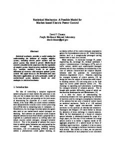
of A. Thus how well two orthogonal signal can be resolved may be dependent on the system size N as well as the separation between signal strengths. Figure 1共d兲 shows theoretical and simulation learning curves for a population covariance that contains three signal directions. Although the first two signal strengths are identical to those in Fig. 1共a兲 and the retarded learning transition points are equally spaced, the effect of the third signal direction on the learning curve for the second principal component is very apparent when comparing Figs. 1共a兲 and 1共d兲. This is an issue we address in the next section. V. FLUCTUATION EFFECTS

For the theoretical analysis given in Sec. III A and III B we have taken the eigenvalues of C to be nondegenerate, so −2 the sigthat above the retarded learning transition at ␣ = Am nal direction Bm is learnt to some degree by the mth principal component Jm. We can consider for illustrative purposes the leading eigenvalue of C being g-fold degenerate, i.e., A1 = A2 = ¯ = Ag ⬅ ¯A. In the asymptotic limit N → ⬁ we would expect that the first principal component is invariant to rotations within the subspace spanned by the degenerate population eigenvectors. The effective potential in Eq. 共11兲 is a 2 g Rm , and so one has a subspace of stationary function of 兺m=1 points of Eq. 共11兲 given by g

兺

m=1

IV. SIMULATION

Since the asymptotic theory for multiple principal components indicates that the learning curve for the Tth principal component is determined in isolation from the other principal components, we have performed simulations of only the multiple principal component case. Figure 1共a兲 shows learning curves when C contains two symmetry breaking directions, with signal strengths A21 = 20 and A22 = 10. This leads to transitions points at ␣ = 0.05 and ␣ = 0.1 for the first and second principal components, respectively. For these simula2 tions we have set N = 3200 and ␴2 = 1. The overlap values R11 2 and R22 shown are averages estimated from 1000 sample ˆ formed from data drawn from the discovariance matrices C tribution given in Eq. 共1兲. The presence of retarded learning transitions for each of the principal components is clearly present. Figure 1共b兲 shows learning curves for a smaller system size N = 200 with all other parameters as in Fig. 1共a兲. For the smaller system finite size effects are clearly evident, particularly near the transition points predicted by the asymptotic theory in Eq. 共23兲. However, Fig. 1共c兲 demonstrates that the 2 does converge towards the theoretexpectation value for R11 ical asymptotic value as N is increased. At smaller values of N the discrepancy, due to finite size corrections, between the asymptotic theory and simulation is more marked. For small finite systems learning the underlying signal directions is obviously a harder task and we would expect that this is exacerbated for signals with similar strengths, i.e., similar values

2 Rm =

␣¯A2 − 1 ⬅ ⌺共0兲 1 . ¯A共1 + ␣¯A兲

共24兲

2 over the surface of a Taking an average of Rm −1 共0兲 g-dimensional sphere of radius 冑⌺共0兲 1 gives g ⌺1 . From this one would expect the expectation value 具共J · Bm兲2典␰ to be g−1⌺共0兲 1 . One may question the likelihood of encountering a situation where the population covariance eigenvalues are precisely degenerate. Of more realistic interest is the case where two 共or more兲 eigenvalues of C are similar in value. For illustration purposes we can consider the two symmetry breaking direction case, i.e., S = 2. Above the appropriate retarded learning transitions, for sufficiently large N any difference A1 − A2 ⬎ 0 will result in the first principal component J1 learning the signal direction B1. This leads us naturally to consider the behavior of R1 , R2 when ⌬A ⬅ A1 − A2 ⬃ N−␶ , ␶ ⬎ 0 as N → ⬁. For large values of ␶ we would expect to 2 approach the degenerate scenario with Rm → 21 ⌺共0兲 1 , while for smaller values of ␶ we would expect the decrease in ⌬A to be sufficiently slow enough that the increase in N allows for B1 to be learned without confusion by B2, i.e., R21 → ⌺共0兲 1 and R22 → 0 as N → ⬁. When the population covariance C has a rotational invariance we expect this to be reflected in the saddle point structure of the partition function given in Eq. 共10兲. Consequently the Hessian will be nearly singular for the near-degenerate scenario. Under these circumstances critical- like fluctuations will mean that the Hessian provides a contribution to the effective potential similar in magnitude to that given by the leading order 共tree level兲. The effect of a nearly degenerate

016101-5



FIG. 1. 共a兲 Learning curves, at fixed N = 3200, for the first two principal components. The population covariance contains two symmetry breaking directions, with A21 = 20, A22 = 10, and we have set ␴2 = 1. Simulation values 共solid symbols兲 are averages over 1000 data sets. The solid and dashed lines represent the theoretical results given by Eq. 共23兲. Standard errors of the simulation averages are less than the size of the plotted symbols. 共b兲 Learning curves, at fixed N = 200, for the first two principal components. All other parameters as the same as for Fig. 1共a兲. 共c兲 Convergence to the asymptotic value of R211, at fixed ␣ = 0.2. The asymptotic value predicted by Eq. 共23兲 is denoted by the horizontal dashed line, while the solid symbols represent simulation averages over 1000 data sets. Standard errors of the simulation averages are less than the size of the plotted symbols. The inset shows simulation estimates of the sample variance for R211. 共d兲 Learning curves, at fixed N = 3200, for the first three principal components. The population covariance contains three symmetry breaking directions, with A21 = 20, A22 = 10, A23 = 20/ 3 = 1 / 0.15. Other parameters and simulation settings are as for 共a兲.

population covariance can be determined by considering the fluctuation contribution to the effective potential. The relevant expression for the replica symmetric effective potential, to leading order in n␤ 共see Appendix B兲, is ⌫ = ⌫tree + ⌫fluc with

冉

t= 1− and dm = t

⌫tree = − Nn␤␴2t2 ,

n ⌫fluc = ␤␴2 2

where

冤

兺m

−1 C共Am兲dm

−兺 m

共25兲

2 2 −2 C共Am兲Rm f 共Am兲dm

1 + 兺 Rm⬙ f 2共Am⬙兲dm⬙ 2

m⬙

−1

冥

,

共26兲

冋冉

兺

2 Rm

m=1

2 1 − 兺 Rm m

冊冉冋 1/2

S

冊

S

+ ␣ 1+

−1/2

兺

2 A mR m

m=1

冉

册冊

2 − ␣1/2Am 1 + 兺 AmRm m

1/2

共27兲

冊册 −1/2

. 共28兲

The functions f共Am兲 and C共Am兲 are defined by Eqs. 共B9兲 and 共B11兲 in Appendix B. Note that these expressions are valid S is for all S 艌 2. The behavior of the order parameters 兵Rm其m=1 determined by minima of ⌫. Setting Am = ¯A + ⌬Am we consider the limit ⌬Am → 0. Small values of ⌬Am will lead to the fluctuation contribution in Eq. 共26兲 being significant at finite values of N. The relative sizes of ⌬Am and N then become 2 . To consider the important in determining the behavior of Rm

016101-6



finite size effects of nearly degenerate signals we set ˜ N−␶. In the limit N → ⬁ the functions f共A 兲 and ⌬Am = ⌬A m m C共Am兲 tend to finite nonzero limiting values that depend only on ¯A. We separate out the asymptotic values of the order param2 2 = Rm,0 + ⌬Sm, eters and so decompose minima of ⌫ as Rm 2 S where 兵Rm,0其m=1 is any set of values which satisfies 兺mRm,0 共0兲 = ⌺1 . We have ⌬Sm → 0 as N → ⬁, and so write ⌬Sm ˜ N−␦. Similarly, for fixed 兵⌬A ˜ 其S we have d → 0. If = ⌬S m m m=1 m −␦d ˜ we write dm = dmN then ⳵⌫fluc / ⳵Rm is dominated by derivatives with respect to dm, and is O共N−1+2␦d兲. Noting that dm −1 2 = −Rm ⳵t / ⳵Rm then for Rm2 ⬎ 0 we can express ⳵⌫tree / ⳵Rm and the dominant contribution to ⳵⌫fluc / ⳵Rm in terms of 兵dm其. From this we immediately have that ␦d = 31 . For ␶ ⬍ 31 the tree level contribution to ⳵⌫ / ⳵Rm is dominant over the fluctuation contribution and can be expanded to leading order as

− 2Nn␤␴ t0Rm,0 2

冤

not constant over m are smaller than O共N−␶兲, and so the O共⌬Am兲 term in Eq. 共29兲 cannot be balanced for ␶ ⬎ 31 , even though it is subdominant. Consequently for ␶ ⬎ 31 we have that ⳵⌫ / ⳵Rm = 0 does not admit a perturbative solution about 2 兵Rm,0 其. For ␶ ⬎ 31 we can find a minimum of ⌫ by constrain2 to a common identical value, R2, and minimizing ing all Rm with respect to R2. Clearly for this minimum we have R2 → g−1⌺共0兲 1 . The leading order contribution to ⌫ comes from the tree level and is −Nn␤␴2t20, with next to leading contributions from both fluctuations and the tree level being O共N−1/3兲. Consequently, the asymptotic behavior of the overlap order parameters, deduced from our analysis of the effective potential ⌫, is summarized below.

lim R21 =

兺 ⌬Sm⬘ 1 m⬘ ␣1/2⌬Am + 共0兲 3/2 共1 + ¯A⌺共0兲兲1/2 2 共1 − ⌺1 兲 1

¯ ⌬S + ⌬A R2 兲 ␣ A 兺共A m⬘ m⬘ m⬘,0 1/2¯

−

␦ = 31 . Other terms from ⳵⌫tree / ⳵Rm and ⳵⌫fluc / ⳵Rm that are

m⬘

3/2 2共1 + ¯A⌺共0兲 1 兲

冥

+ O共N

−2 min共␶,␦兲

N→⬁

2 = lim Rm

N→⬁

兲. 共29兲

From Eq. 共29兲 we can see that since the second and third −1 ⳵⌫tree / ⳵Rm are independent of m then terms in Rm ⳵⌫tree / ⳵Rm = 0 , ∀ m iff Rm,0 ⬅ 0 for all but one value of m. 2 is nonzero is as yet Which of the asymptotic values Rm,0 undetermined. The tree level effective potential is given by

冤

⌫tree = − Nn␤␴2 t0 + N−␶␣1/2

冥

2 兺m ⌬A˜mRm,0 1/2 共1 + ¯A⌺共0兲 1 兲

2

+ O共N−2 min共␶,␦兲兲 ,

共30兲

¯ , 兵R 其兲. Consequently we are free to minimize where t0 = t共A m,0 the tree level effective potential with respect to Rm,0 subject 2 to the constraint 兺mRm,0 = ⌺共0兲 1 . The largest positive value of ˜ will occur at m = 1 and so, as N → ⬁, Eq. 共30兲 will be ⌬A m 2 2 minimized by setting R1,0 = ⌺共0兲 1 , and Rm,0 = 0 , ∀ m ⬎ 1. So even for an asymptotically degenerate population covariance, if ␶ ⬍ 31 the leading signal direction will be learnt with the same efficiency as for a nondegenerate population covariance. This is hardly surprising given that for ␶ ⬍ 31 and finite N we are minimizing ⌫ by minimizing ⌫tree, as we would for the asymptotic theory. The sum of leading order corrections 兺m⌬Sm is then determined from Eq. 共29兲 by balancing the O共⌬A1兲 contribution in Eq. 共29兲, to give ␦ = ␶. For ␶ ⬎ 31 the dominant contribution to ⳵⌫ / ⳵Rm is O共N−1/3兲 from the fluctuation term. This is balanced by the second and third terms in Eq. 共29兲, and so for this scenario

冦

g

冦

⌺共0兲 1 , g

−1

⌺共0兲 1 ,

␶⬍

1 ␶⬎ 3 1 3

0,

␶⬍

⌺共0兲 1 ,

1 ␶⬎ 3

−1

1 3

冧

,

冧

,

m 艌 2.

共31兲

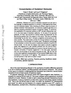
Figure 2 shows simulation results for the two symmetry breaking direction case, i.e., S = 2. We have set ¯A = 21 共冑20 + 冑10兲, ␴2 = 1 and ␣ = 0.2 so that we are above the retarded learning transition point for ¯A. Figure 2共a兲 shows 2 for different values of ␶, while convergence with N of R11 2 for different values of Figure 2共b兲 shows convergence of R12 2 ␶. For small values of ␶, e.g., ␶ = 0.1, the convergence of R11 共0兲 towards the asymptotic value ⌺1 is clear. Despite the approach to a twofold degenerate population covariance the stronger signal direction B1 is learnt without confusion by 2 B2. For intermediate values of N we in fact have R11 ⬎ ⌺共0兲 1 since A1 ⬎ ¯A for these intermediate values of N. For larger 2 converging values of ␶, e.g., ␶ = 0.5 and ␶ = 1 we have R11 1 共0兲 towards 2 ⫻ ⌺1 . Although we have not explicitly given the analysis of fluctuations for the multiple principal component case the intuitive picture presented here suggests that, due to the orthogonality of the signals and the decomposition, the conclusions presented will still be valid for multiple principal components and when we have a population covariance containing more than one near-degenerate subspace. Figure 3 shows simulation results for a population covariance with four symmetry breaking directions. The first two signals are nearly degenerate with A1 − A2 ⬃ N−1 and 1 1 冑冑 2 共A1 + A2兲 = 2 共 20 + 10兲, while the third and fourth signals are nearly degenerate with A3 − A4 ⬃ N−0.1 and 21 共A3 + A4兲 = 21 共冑1 / 0.3+ 冑1 / 0.35兲. From our analysis of the one principal component problem we would expect the first principal component J1 to overlap with the signal directions B1 and B2 2 2 2 equally well, i.e., R11 ⯝ R22 ⯝ R12 ⯝ R21 as N → ⬁. In contrast learning of the third signal direction by the third principal

016101-7



FIG. 2. Plots of overlaps R2 between the first principal component and the signal directions for different system sizes N. We have fixed ␣ = 0.2 and set ␴2 = 1. The population covariance contains two signal directions with similar signal strengths A1 = ¯A + ⌬A , A2 = ¯A − ⌬A. The signal strength separation is an increasingly weak function of N, i.e., ⌬A ⬃ N−␶ , ␶ ⬎ 0. The solid symbols show simulation averages for different values of ␶. Simulation averages are over 1000 data sets, except for the largest value of N for which simulation averages are over 100 data sets. 共a兲 Plot of R211. The upper dashed line shows the asymptotic value of R211 predicted by Eq. 共23兲 for A1 = ¯A, while the lower dashed line is drawn at half this value. 共b兲 Plot of R212. The dashed line is drawn at half the asymptotic value of R211 predicted by Eq. 共23兲 for A1 = ¯A.

component should be unaffected by the presence of the 2 = 共␣A23 − 1兲 / 关A3共1 + ␣A3兲兴 fourth signal direction, i.e., R33 and R44 → 0, as N → ⬁. From Fig. 3共a兲 it is clear that the presence of the second signal component B2 is affecting the accuracy of the first principal component J1 in representing the first signal component B1. In contrast Fig. 3共b兲 shows that with increasing N the fourth signal component B4, has a decreasing effect upon the accuracy of the third principal component J3. VI. DISCUSSION AND CONCLUSIONS

In this paper we have utilized ideas and techniques from statistical physics to understand the accuracy with which sig-

FIG. 3. Plot of R2 for the first and third principal components. We have fixed ␣ = 0.5 and set ␴2 = 1. The population covariance C contains four signal directions. A1 and A2 are of similar strength, with A1 − A2 ⬃ N−1, while A3 and A4 are of similar strength, with A3 − A4 ⬃ N−0.1. The solid symbols show averages over 1000 simulated data sets for different values of N. 共a兲 shows R211 and R212. The dashed line shows the common predicted asymptotic value of R211 and R212. 共b兲 shows R233 and R234. The dashed line shows the predicted asymptotic value of R233.

nals, or patterns, within data are detected. Specifically, our aim was the study of the principal component learning curves for high dimensional data. The learning curve for each principal component displays a separate phase transition that coincides with the phase transition in the sample covariance eigenspectrum, whereby a single eigenvalue detaches from the bulk spectrum 关10兴. That the series of phase transitions in the learning curve and eigenspectrum coincide is hardly surprising. Equally the fact that the form of the learning curves are determined by a single functional form, with only the value of Am differing, ultimately stems from the orthogonal decomposition nature of PCA. A number of the findings that have been determined using statistical physics techniques have begun to be put on a more rigorous mathematical and statistical footing. For example, Péché 关20兴 demonstrates the universality of the Marčenko and Pastur form for the bulk spectrum 关21兴 when the signal S are sufficiently weak. Similarly Paul 关22兴 strengths 兵Am其m=1

016101-8



has also derived the existence of retarded learning transitions for multiple principal components within the symmetry breaking model considered in this paper, while Baik et al. 关16兴 study the distribution of the largest sample covariance eigenvalue in the symmetry breaking direction model when the signal strengths are large. Baik and Silverstein 关23兴 determine the eigenvalue spectrum of a population covariance equivalent to that studied here, confirming the results obtained by Hoyle and Rattray using statistical physics techniques 关10兴. Simulation results presented in Fig. 2 focus on the two symmetry breaking direction case. Naively one might assume that when the distributions of the largest two sample covariance eigenvalues effectively overlap, then the two signal directions will be effectively indistinguishable 共degenerate兲 and the degree to which they are learnt, as measured by 2 2 and R22 , will be reduced. Although the order parameters R11 for the isotropic case the distribution of the largest sample covariance eigenvalue, ␭1 is known to follow a TracyWidom distribution, with its characteristic N−2/3 scaling of the standard deviation 共in contrast to a N−1/2 scaling expected from a standard central limit argument兲, the work of Baik et al. 关16兴 indicates that above the corresponding retarded learning transitions an N−1/2 scaling is appropriate, suggesting that the distributions of ␭1 and ␭2 will certainly overlap when A1 − A2 ⬃ N−1/2. Critical-like fluctuations that result from the near degeneracy may renormalize this exponent and effective overlap between ␭1 and ␭2 will occur for larger values of A1 − A2. However, for the near degenerate scenario A1 , A2 → ¯A, both ␭1 and ␭2 are attempting to learn the same population eigenvalue ␴2共1 + ¯A兲, and so the approaching degeneracy need not cause significant added difficulty in learning the population eigenvalue. In contrast, in the limit A1 , A2 → ¯A the actual signal directions will be defined only up to an arbitrary rotation within the degenerate subspace, 2 and resulting in greater variance of the fluctuations of R11 2 R22. This is essentially the mechanism deduced in Sec. V. If A1 − A2 ⬃ N−␶ and ␶ ⬎ 31 , then as we approach the thermodynamic limit N → ⬁, N does not grow fast enough to suppress fluctuations within the subspace spanned by the nearly degenerate signal directions, and so the leading principal components become oblivious to the weak structure within the data. This conclusion is valid irrespective of the asymptotic value ¯A of the signal strength provided we are above the retarded learning transition, i.e., ␣ ⬎ ¯A−2. Ultimately, if ⌬A is the separation of two population eigenvalues, then unless ⌬A Ⰷ N−1/3, the two population eigenvalues will be effectively degenerate from the point of view of the sample data and the sample covariance. This relatively weak decrease with N means that even in what we may naively think of as large systems, for which we believe the asymptotic theory to be accurate, the effect of fluctuations can be marked. The 2 effect can be demonstrated by contrasting the behavior of R22 in Figs. 1共a兲 and 1共d兲. In Fig. 1共a兲 the top two signals are well separated 共A1 − A2 ⯝ 1.31兲 and simulation results follow closely the theoretical learning curves. However, in Fig. 1共d兲 the addition of a third signal which is closer to the second signal 共A2 − A3 ⯝ 0.58兲 increases noticeably the discrepancy

2 between simulation and asymptotic theory for R22 , even though the retarded learning transition points are equally spaced in ␣ and N is large 共N = 3200兲. How much insight do we gain from analysis of fluctuation effects in the leading principal component? We have not given here the full analysis of fluctuation effects for multiple principal components since it is considerably more involved. Although the theoretical analysis given in Sec. V concentrates on the behavior of the leading principal component, we would expect the conclusions to be valid for the multiple principal component case. Indeed the simulation results presented in Fig. 3 suggest that this is the case. The impact of finite size effects for multiple principal components is also likely to extend beyond the batch learning scenario with ␣ ⬍ 1 that we have primarily discussed here. Significant finite size effects will have repercussions for online training scenarios, even though by definition online training considers an increasing number of presented training examples and therefore studies the approach to accurate learning of the true signal directions from a potentially large number of training examples 共␣ Ⰷ 1兲关11,12兴. In the initial stages of online learning the principal components have yet to learn the true signal directions. Any one particular principal component will represent all the true signal directions almost equally poorly. The system thereby displays a permutation symmetry. As training progresses this permutation symmetry is broken, with individual principal components specializing in learning a particular signal direction. One would suspect that this dynamical symmetry breaking is intricately linked to the presence of retarded learning phase transitions in the batch learning scenario. Such an observation has been commented on by Bunzmann et al. who used a PCA decomposition of training data as a prior input stage to an artificial neural network, with training of the principal components and neural network performed simultaneously online 关13兴. The putative link between dynamical symmetry breaking in online learning and retarded learning phase transitions in batch learning emphasizes the importance of the finite-size effects studied within this paper. Critical-like fluctuations arising from nearly degenerate signals that lead to renormalization of the leading order mean-field theory will most likely also lead to critical slowing down of online learning, with an extended “plateau” stage in the PCA learning curve within the online learning scenario considered by Biehl and Schlösser 关11兴. The work of Bunzmann et al. highlights that PCA may be used as a prior step to more sophisticated learning algorithms, or implicitly within those learning algorithms. Understanding how orthogonal decompositions of sample data perform is then a key component in understanding the performance of these composite learning algorithms.

ACKNOWLEDGMENTS

D.C.H. would like to acknowledge the MRC 共U.K.兲 for financial support. We would like to thank Mr. David Nuttall for help with some of the larger, computationally intensive calculations. APPENDIX A

One principal component. Here we set T = 1 and denote the single principal component by J. We wish to evaluate the ensemble average

016101-9


冓冕 ln

冉

p

dJ␦共1 − 储J储兲exp ␤ 兺共␰␮ · J兲 + 2

2

␮=1

S

兺 h mJ · B m m=1


冊冔

. ␰

共A1兲

Ultimately we take the limit hm → 0+. The leading order 共tree level兲 expression for the effective potential can be determined from the saddle point structure of the appropriate partition function in the absence of hm. Therefore, for convenience we shall drop the source terms from subsequent expressions. We start with the replica partition function Z = 共2␲兲

−N p/2

冉

⫻exp −

冉

共det C兲

−

冕兿冊冕兿 ␮=1

␯

dR␯

␯⬘⬎␯

␯=1

dJ

␯=1

兿 ␦共1 − 储J␯储2兲共det M兲−p/2 , 共A3兲

T 兲, where 共for C = ␴2I + ␴2兺mAmBmBm

M ␯␯⬘ = ␦␯␯⬘ − 2␤␴

2

冉

S

q␯␯⬘ +

兺 AmRm␯ Rm␯⬘ m=1

冊

␯⬘ ⫽ ␯,

∀ ␯,

∀ ␯.

q␯␯ = 1,

再冋

册

S

冋

S

冓冕

冉

T

T

p

dJi␦共IT − K兲exp ␤ 兺兺共␰␮ · Ji兲2 兿 i=1 ␮=1 i=1

ln

共A4兲

冕兿 ␯

冕兿兿冕兿 dJ␯

␯=1

␯

⫻

␯⬘⬎␯

␦共1 − 储J␯储2兲

共det C兲

冕兿 ␯

␯ dRm ␦共Rm␯ − J␯ · Bm兲

dq␯␯⬘␦共q␯␯⬘ − J␯ · J␯⬘兲.

共A5兲

We rewrite ␦ functions in terms of their Fourier representations. After integrating over J␯ and Fourier variables, and

−

p 2

冊冔

, ␰

共A9兲

冕兿 p

␮=1

d␰␮

冉冊冕兿兿冉兺兺兺冊 p

1 ⫻exp − 兺 ␰␮T C−1␰␮ 2 ␮=1 T

␯ 2

n

=

Z = 共2␲兲

−N p/2

⫻ exp ␤

兿 ␦共1 − 储J 储兲 ␯=1

.

where Kii⬘ = Ji · Ji⬘. Introducing replicas for the principal components J1 , J2 , . . . , JT we obtain the replica partition function

n

dJ

册冎

In the limit N → ⬁ the integral in Eq. 共A6兲 is dominated by stationary points of Eq. 共A8兲 and to leading order ln Z is simply the value of the exponent in Eq. 共A8兲. At this order 共tree level兲 the effective potential is identical in form to the 2 now repnegative of the saddle point exponent, but with Rm 2 resenting the order parameter 具共J · Bm兲典␰, rather than an integration variable. Multiple Principal Components. For multiple principal components 共T ⬎ 1兲 the appropriate expectation value is

,

␯ Here we have abused the notation by using Rm to represent the overlap between the ␯th replica of the first principal component J␯ and the signal direction Bm, while we also use 2 to represent the expectation value 具共J · Bm兲2典␰. However, it Rm will always be apparent in which context we are using the notation. The integrations over J␯ are performed in terms of ␯ and q␯␯⬘, i.e., integrations over Rm ␯

共A7兲

共A8兲

␯ = J␯ · Bm , Rm

q␯␯⬘ = J␯ · J␯⬘ .

,

∀ ␯,

2␣ 1 1 2 2 Nn␤␴2 1 − 兺 Rm + 1 + 兺 A mR m 2 x 1 − 2x m=1 m=1

共A2兲

␯=1

␯=1

冊册

Putting x = ␤␴2共1 − q兲 then, to leading order in n␤ the exponent of the integrand becomes

dJ␯ 兿 ␦共1 − 储J␯储2兲

n

␯

1 ␣ tr ln L − tr ln M 2 2

S ␯ ␯⬘ RmRm . We now look for stationwhere L␯␯⬘ = L␯⬘␯ = q␯␯⬘ − 兺m ary points of the exponent of the integrand in Eq. 共A6兲. Assuming replica symmetry for such saddle points we put,

q␯␯⬘ = q, n

We can rewrite exp关␤共J␯ · ␰␮兲2兴 as 共1 / 冑2␲兲兰 dx␯␮ ⫻exp共− 21 x␯2␮ + ␤1/2x␯␮J␯ · ␰␮兲. After integrating over ␰␮ and x␯␮ we obtain n

冋冉

dq␯␯⬘ exp N

共A6兲

d␰␮ n

冊

␮,␯

冕兿

冕兿冕兿

␯ Rm = R m,

⫻ exp ␤ 兺共J␯ · ␰␮兲2 .

Z = 共2␲兲

Z⯝

p

p 2

1 兺 ␰T C−1␰␮ 2 ␮ ␮

−共1/2兲Nn

retaining only terms in the exponent of the integrand that are ␯ extensive in N and depend upon 兵q␯␯⬘其 or 兵Rm 其, we obtain

p

n

T

i=1 ␯=1

n

dJi␯

兿 ␦共IT − K␯兲

␯=1

n

i=1 ␮=1 ␯=1

共Ji␯ · ␰␮兲2 .

共A10兲

Here, the matrix K␯ has elements 共K␯兲ii⬘ = Ji␯ · J␯i⬘⬘. Following the same approach as before it is an easy matter to confirm that Z⯝

冕兿

m,i,␯

␯ dRmi 兿

兿

i,i⬘ ␯⫽␯⬘

冉

dQii⬘⬘ exp ␯␯

冊

N 共tr ln L − ␣tr ln M兲 , 2 共A11兲

where M = I − 2␤P and

016101-10


再冋

␯ Pii⬘⬘ = ␴2Qii⬘⬘ + ␴2 兺 AmRmi Rmi⬘ ⬘ , ␯␯

␯␯

␯

␯ Rmi⬘ ⬘ , Lii⬘⬘ = Qii⬘⬘ − 兺 Rmi ␯␯

␯

+

Qii⬘⬘ = Ji␯ · Ji⬘⬘ . ␯

␯␯ Qii⬘⬘ =

∀ ␯, ∀ ␯ ⫽ ␯⬘ .

qii⬘,

+

共A12兲

␯ = Ji␯ · Bm represents the overlap of the ␯th replica of Here Rmi the ith principal component, Ji with the mth symmetry breaking direction Bm. Under an assumption of that dominant saddle points of the integrand in Eq. 共A11兲 are replica symmetric we put ␯ Rmi = Rmi,

再冋冉冋

冉

冊册

T + 2␣tr 共I − 2X兲−1 I + 兺 AmRmRm m

共Rm兲i = Rmi , 共q兲ii⬘ = qii⬘ .

再冋

册

S

冋

S

2␣ 1 1 2 2 Nn␤␴2 1 − 兺 Rm + 1 + 兺 A mR m 2 x 1 − 2x m=1 m=1 +

册冎

N 兺 ␦Rm␯ ␦Rm␯⬘⬘关H共RR兲 2 m,m ,␯,␯ ⬘

⬘

− 共H共qR兲兲T共H共qq兲兲−1H共qR兲兴m,m⬘,␯␯⬘ 1 n共n − 1兲 N ln − tr ln共− H共qq兲兲 − . 2 4 2␲

,. 共A14兲

共B3兲

The matrix H共qq兲 has the form 共A15兲

共qq兲

H␥␥⬘ = C0 + C1␦␥1␥⬘␦␥2␥⬘ + C2共␦␥1␥⬘ + ␦␥2␥⬘ + ␦␥1␥⬘ + ␦␥2␥⬘兲, 1

2

1

2

2

1

共B4兲

共A16兲共A17兲

and so is of the form considered by de Almeida and Thouless 关1,24兴. Eigenvalues of H共qq兲 are then easily determined. Explicitly we find to O共n␤兲, ln det共− H共qq兲兲

APPENDIX B

For simplicity and illustrative purposes we only analyze fluctuation effects for the one principal component case. The one-loop contribution to the effective potential is given by evaluating ln det共−H兲 for the Hessian H of the tree level saddle point and simply replacing the saddle point value of 2 with the order parameter 具共J · Bm兲2典␰. Since we use the Rm 2 same notation Rm to represent the integration variable and the order parameter we have only to express ln det共−H兲, evaluated at the saddle point, entirely in terms of the saddle point value of Rm. We start from exponent of Eq. 共A6兲 N N␣ tr ln L − tr ln M. 2 2

共B2兲

⬘

We have decomposed the Hessian into the various contributions from 共i兲 just fluctuations ␦q␯,␯⬘, 共ii兲 just fluctuations ␦Rm␯ , 共iii兲 cross terms involving both ␦q␯␯⬘ and ␦Rm␯ . For brevity, we do not give here the expressions for the matrices H共qq兲 , H共qR兲 , H共RR兲, since they are easily evaluated. The Gaussian fluctuations in ␦q␥ are easily integrated out to yield

where Rm and X are defined by X = ␤␴2共I − q兲,

⬘ ⬘

⬘

共A13兲

冊册冎

册冎

N 共RR兲 ␦ R ␯⬘ . 兺 ␦Rm␯ Hm,m ⬘,␯␯⬘ m⬘ 2 m,m ,␯,␯

To leading order we obtain the exponent of the integrand for a replica symmetric configuration as 1 T Nn␤␴2 tr X−1 I − 兺 RmRm 2 m

冋

S

N ␯⬘ 兺 ␦q␥H␥␥共qq兲⬘ ␦q␥⬘ + N 兺 ␦q␥H␥共qR兲 m⬘,␯⬘␦ R m⬘ 2 ␥,␥ ␥,m ,␯ ⬘

m

␯␯

册

S

1 2␣ 1 2 2 + Nn␤␴2 1 − 兺 Rm 1 + 兺 A mR m 2 x 1 − 2x m=1 m=1

m

␯␯


共B1兲

We simplify the notation by using ␥ = 共␯ , ␯⬘兲 = 共␥1 , ␥2兲 to represent an ordered pair of replicas ␯⬘ ⬎ ␯. Denoting fluc␯ and ␦q␯,␯⬘ = ␦q␥ we tuations, in an obvious notation, as ␦Rm can expand Eq. 共B1兲 about a replica-symmetric saddle point to obtain 共to second order兲,

= n␤␴2

⫻

冋

冋

冉

冉

2 1 − 兺 Rm m

x4

2 1 − 兺 Rm m

x3

冊

2

− 16␣

冊冉 + 8␣

冉

2 1 + 兺 A mR m m

冊

共1 − 2x兲4

2 1 + 兺 A mR m m

共1 − 2x兲3

⫻关1 + O共␤−1兲兴.

冊

册

2

册

−1

共B5兲

It can be verified that the inverse of H共qq兲 is also of the form given in Eq. 共B4兲 above. Substituting the form in Eq. 共B4兲 into Eq. 共B3兲 gives H共RR兲 − 共H共qR兲兲T共H共qq兲兲−1H共qR兲 ⬅ −U, with U of the form U = W␦␯␯⬘ + 1n1Tn Y,

共B6兲

where 1n represents an n-dimensional vector in replica space with components all equal to 1. Finally integrating out ␯ gives a contribution of Gaussian fluctuations in ␦Rm

016101-11



from ntrW−1Y in 共B7兲. The inverse matrix W−1 is easily evaluated as,

1 Sn ln 2␲ − tr ln NU + 2 2 =−

冉

冊

n N tr ln W + tr关W−1Y兴 + S ln + O共n2兲. 2 2␲

冤

共B7兲 2 2 Using notation ⌺1 = 兺mRm and ⌺2 = 兺mAmRm , one explicitly finds

冋

册

1 2␣Am − + 8␤␴2RmRm⬘ f共Am兲f共Am⬘兲 Wmm⬘ = ␤␴ ␦mm⬘ x 1 − 2x 2

共B8兲

+ O共n兲, where the function f共Am兲 is given by f共Am兲 =

冋

4␣Am 1 2 + x 共1 − 2x兲2

册冋

1 − ⌺1 8␣共1 + ⌺2兲 + x3 共1 − 2x兲3

册

−1

−1 − 关W−1兴mm⬘ = ␤−1␴−2 ␦mm⬘dm

m⬙

ntrW−1Y = n␤␴2

冤

兺 C共Am兲dm−1 − 兺 m

m

2

−

兺

册

4␣Am共1 + ⌺2兲 1 − ⌺1 + . 共1 − 2x兲2 x2

dm = t

Similarly we decompose g共Am , Am⬘ , x , ⌺1 , ⌺2兲 = g0 − 16共g1 + g2兲 / g4 − 16g3 / g24 where, 1 4 ␣ A mA m⬘ − , x2 共1 − 2x兲2

共B12兲

册

4␣Am 1 2 + x 共1 − 2x兲2

册冋

4 ␣ A m⬘ 1 , 2 + x 共1 − 2x兲2

册

1 − ⌺1 8␣Am⬘共1 + ⌺2兲 − , x3 共1 − 2x兲3 共B14兲

g3 =

册冋册

冋

4␣Am 1 2 + x 共1 − 2x兲2

−

16␣共1 + ⌺2兲2 , 共1 − 2x兲4 g4 =

冋

4 ␣ A m⬘ 1 2 + x 共1 − 2x兲2

册冋

共1 − ⌺1兲2 x4 共B15兲

册

1 − ⌺1 8␣共1 + ⌺2兲 + . x3 共1 − 2x兲3

冋冉

1 + 兺 Rm⬙ f 2共Am⬙兲dm⬙ 2

−1

m⬙

2 1 − 兺 Rm

冥

共B16兲

In order to affect the leading order asymptotic calculation we require a contribution of order O共n␤兲. Such terms only come

共B18兲

m

冊

−1/2

冉

2 − ␣1/2Am 1 + 兺 AmRm m

冊册 −1/2

,

共B19兲 where

冉

t= 1−

共B13兲

冋

−1

2 −1 g共Am,Am⬘兲Rm Rm⬘ f共Am兲f共Am⬘兲dm d m⬘

Source terms in Eq. 共10兲 for the evaluation of 具共J · Bm兲2典␰ do not affect the saddle point equation 共12兲 and so we can simply substitute into dm, C,f, and g the tree-level expression for x in terms of the set of order parameters 兵Rm其, i.e., insert the positive root of Eq. 共12兲. For dm this gives

共B11兲

g2 =

−1

+ O共n2兲. 共B10兲

册冋

2

m

+ ␤2␴4g共Am,Am⬘,x,⌺1,⌺2兲RmRm⬘ + O共n兲,

冋

1 + 兺 Rm⬙ f 2共Am⬙兲dm⬙

2 −1 + 兺 Rm g共Am,Am兲dm

−1/2

Y mm⬘ = ␤ ␴ ␦mm⬘C共Am,x,⌺1,⌺2兲

1 − ⌺1 8␣Am共1 + ⌺2兲 − g1 = x3 共1 − 2x兲3

2 2 −2 C共Am兲Rm f 共Am兲dm m⬙

2 4

g0 =

冥

共B17兲

m,m⬘

冋

−1

2

where dm = x−1 − 2␣Am共1 − 2x兲−1. Evaluating ntrW−1Y gives

and

C共Am,x,⌺1,⌺2兲 = −

1 + 兺 Rm⬙ f 2共Am⬙兲dm⬙

+ O共n兲,

共B9兲

with C共Am , x , ⌺1 , ⌺2兲 given by

−1 RmRm⬘ f共Am兲f共Am⬘兲dm d m⬘

兺

m=1

冊冉冋 1/2

S

2 Rm

+ ␣ 1+

S

兺

m=1

2 A mR m

册冊

1/2

. 共B20兲

The 共one-loop兲 fluctuation contribution to the determination of the order parameter 具共J · Bm兲2典 then comes from differentiating Eq. 共B18兲 with respect to Rm. We are specifically interested in the near degenerate scenario, for example, when two signal strengths are similar in value. Under this scenario the Hessian of Eq. 共B1兲 will be nearly singular and we expect a divergent contribution from tr ln U. We can write Am = ¯A + ⌬Am. In the limit Am → ¯A ∀ m, we have that dm → 0. In this limit the contribution from ln det共−H共qq兲兲 given in Eq. 共B5兲 is finite, and so we no longer consider it. The dominant ⳵d−1 terms in limn→0 ⳵R⳵ m trW−1Y come from derivatives ⳵Rmm . We find derivatives, with respect to dm, of the third and fourth terms in Eq. 共B18兲 cancel to leading order in the limit ⌬Am → 0, for all values of the order parameters 兵Rm其. Therefore we concentrate on the first and second terms to determine the order parameter values 兵Rm其 in the limit Am → ¯A, i.e., the relevant, dominant contribution to the effective potential from fluctuations is

016101-12



冤

2 2 −2 C共Am兲Rm f 共Am兲dm

冥

In contrast the tree level contribution is O共nN␤兲. There are also additional O共n␤兲 contributions from next-to-leading

order terms omitted from the integration over Fourier variables in Eq. 共A5兲. However, these omitted contributions do not explicitly depend upon the signal strengths Am, and it is easily confirmed that the omitted terms remain finite in the degenerate limit ⌬Am → 0. Consequently they are subdominant in comparison to the contribution in Eq. 共B21兲 and we no longer consider them.

关1兴 A. Engel and C. Van den Broeck, Statistical Mechanics of Learning 共Cambridge University Press, Cambridge, 2001兲. 关2兴 A. M. Tulino and S. Verdu, Random Matrix Theory and Wireless Communication, Vol. 1 of Foundations and Trends in Communication and Information Theory 共Now Publishers, Boston, 2004兲. 关3兴 J. W. Silverstein and P. L. Combettes, IEEE Trans. Signal Process. 40, 2100 共1992兲. 关4兴 R. Müller, IEEE Trans. Inf. Theory 48, 2495 共2002兲. 关5兴 V. Plerou, P. Gopikrishnan, B. Rosenow, Luis A. Nures Amaral, T. Guhr, and H. E. Stanley, Phys. Rev. E 65, 066126 共2002兲. 关6兴 T. L. H. Watkin and J.-P. Nadal, J. Phys. A 27, 1899 共1994兲. 关7兴 M. Biehl and A. Mietzner, J. Phys. A 27, 1885 共1994兲. 关8兴 P. Reimann, C. Van den Broeck, and G. J. Bex, J. Phys. A 29, 3521 共1996兲. 关9兴 P. Reimann and C. Van den Broeck, Phys. Rev. E 53, 3989 共1996兲. 关10兴 D. C. Hoyle and M. Rattray, Phys. Rev. E 69, 026124 共2004兲. 关11兴 M. Biehl and E. Schlösser, J. Phys. A 31, L97 共1998兲. 关12兴 E. Schlösser, D. Saad, and M. Biehl, J. Phys. A 32, 4061

共1999兲. 关13兴 C. Bunzmann, M. Biehl, and R. Urbanczik, Phys. Rev. E 72, 026117 共2005兲. 关14兴 I. M. Johnstone, Ann. Stat. 29, 295 共2001兲. 关15兴 C. A. Tracy and H. Widom, Commun. Math. Phys. 177, 727 共1996兲. 关16兴 J. Baik, G. Ben Arous, and S. Péché, Ann. Probab. 33, 1643 共2005兲. 关17兴 R. Urbanczik, Europhys. Lett. 64, 564 共2003兲. 关18兴 C. Itzykson and J.-M. Drouffe, Statistical Field Theory 共Cambridge University Press, Cambridge, 1989兲, Vol. 1. 关19兴 D. C. Hoyle and M. Rattray, Europhys. Lett. 62, 117 共2003兲. 关20兴 S. Péché, Ph.D. thesis, Ecole Polytechnique Fédérale de Lausanne 共2003兲. 关21兴 V. A. Marčenko and L. A. Pastur, Math. USSR. Sb. 1, 507 共1967兲. 关22兴 D. Paul 共unpublished兲. 关23兴 J. Baik and J. W. Silverstein J. Multivariate Anal. 共to be published兲. 关24兴 J. R. L. de Almeida and D. Thouless, J. Phys. A 11, 983 共1978兲.

1 n␤␴2 2

兺 C共Am兲dm−1 − 兺 m

m

兺 m⬙

2 −1 Rm⬙ f 2共Am⬙兲dm⬙

.

共B21兲

016101-13