73 Statistical Mechanics of On-line Node-perturbation Learning. Fig. 1 Network structure of teacher (left) and student (right) networks, both with the same network ...
IPSJ Transactions on Mathematical Modeling and Its Applications
Vol. 4
No. 1
72–81 (Jan. 2011)
Regular Paper
Statistical Mechanics of On-line Node-perturbation Learning Kazuyuki Hara,†1 Kentaro Katahira,†2,†3,†4 Kazuo Okanoya†3,†2 and Masato Okada†4,†3,†2 Node-perturbation learning (NP-learning) is a kind of statistical gradient descent algorithm that estimates the gradient of an objective function through application of a small perturbation to the outputs of the network. It can be applied to problems where the objective function is not explicitly formulated, including reinforcement learning. In this paper, we show that node-perturbation learning can be formulated as on-line learning in a linear perceptron with noise, and we can derive the differential equations of order parameters and the generalization error in the same way as for the analysis of learning in a linear perceptron through statistical mechanical methods. From analytical results, we show that cross-talk noise, which originates in the error of the other outputs, increases the generalization error as the output number increases.
1. Introduction Learning in neural networks 1) can be formulated as optimization of an objective function that quantifies the system’s performance. This is achieved by following the gradient of the objective function with respect to the tunable parameters of the system. This optimization is computed directly by calculating the gradient explicitly and updating the parameters by a small step in the direction of the locally greatest improvement. However, computing a direct gradient to follow can be problematic. For instance, reinforcement learning has no explicit form of objective function, so we cannot calculate the gradient. A stochastic gradient-following method to estimate gradient information is proposed for problems where a true gradient is not directly given. Node-perturbation †1 †2 †3 †4
College of Industrial Technology, Nihon University Japan Science Technology Agency, ERATO Okanoya Emotional Information Project Brain Science Institute, RIKEN Graduate School of Frontier Science, The University of Tokyo
72
learning (NP-learning) 2),3) is one of the stochastic learning algorithms. NPlearning estimates the gradient of an objective function by using the change in the objective function in response to a small perturbation. NP-learning can be formulated as reinforcement learning with a scalar reward, and all the weight vectors are updated by using the scalar reward while the gradient method uses the reward vector. Hence, as well as being useful as a neural network learning algorithm, NP-learning can be formulated as reinforcement learning 2),4) or it can be used in a brain model 5),6) . On-line learning in a perceptron has been analyzed by many researchers using statistical mechanics methods and the exact behavior of the system has been depicted 7)–12) . The network used in NP-learning has several outputs, each of which is a learning agent. The agent is treated as a simple linear perceptron 3) . The objective function of NP-learning is the total error of the agents. The error is distributed according to the quantity of noise added to each output. When the output number is one, NP-learning is the same as on-line learning in a perceptron using a gradient descent algorithm (linear perceptron learning). When the output number is more than two, NP-learning can formulated as on-line learning in a linear perceptron with noise (noisy linear perceptron learning) 13),14) . As we will show, NP-learning is a learning method similar to noisy linear perceptron learning, but it has not yet been analyzed using statistical mechanics methods. In this paper, we analyze NP-learning following the analysis of noisy linear perceptron learning through a statistical mechanical method, and derive order parameter equations which depict NP-learning behavior. We then derive the generalization error using order parameters. From our results, we show that the cross-talk noise, which originates in the error of the other outputs, affects the learning performance in NP-learning and our analysis provides a new perspective regarding the analysis of NP-learning. 2. Model In this section, we formulate the teacher and student networks, and an NP-learning algorithm employing a teacher-student formulation. We assume the teacher and student networks receive N -dimensional input x(m) = (m) (m) (x1 , . . . , xN ) at the m-th learning iteration as shown in Fig. 1. Here, we c 2011 Information Processing Society of Japan �
73
Statistical Mechanics of On-line Node-perturbation Learning (m)
dk
=
N �
(m)
∗ wik xi
= wk∗ · x(m) ,
(2)
i=1
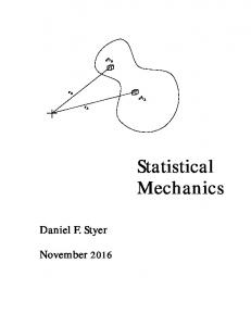
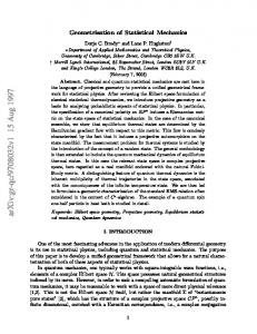
Fig. 1 Network structure of teacher (left) and student (right) networks, both with the same network structure. ξi represents a noise added to i-th student network output.
assume the existence of a teacher network vector wk∗ that produces desired output, so the teacher output dk is a target of the student output yk . The learning iteration m is ignored in the figure. The teacher networks shown in Fig. 1 have N inputs and M outputs, and are identical to M linear perceptrons. Each student network has the same architecture as the teacher. w∗ denotes the weight matrix of teacher networks with M × N elements. w(m) denotes the weight matrix of student networks with M × N elements at the m-th learning iteration, the same as the teacher net(m) works. We also assume that the elements xi of independently drawn input x(m) are uncorrelated random variables with zero mean and variance 1/N ; that is, the i-th element of input is drawn from identical Gaussian distribution P (xi ). In this paper, the thermodynamic limit of N → ∞ is assumed. In the thermodynamic limit, the law of large numbers and the central limit theorem can apply. We can then depict the system behavior by using a small number of parameters. Statistics of the inputs at the thermodynamic limit are as follows. � � � � 1 (m) (m) xi = 0, (xi )2 = , ||x(m) || = 1, (1) N where �·� denotes the average over possible inputs and || · || denotes the norm of a vector. M linear perceptrons are used as the teacher networks and are not subject to learning. Thus, the weight vectors {wk∗ }, k = 1, . . . , M are fixed in the learning (m) process. The output of the k-th teacher dk for N -dimensional input x(m) at the m-th learning iteration is
∗ ∗ where teacher weight vectors {wk∗ }, wk∗ = (w1k , . . . , wN k ) are N -dimensional ∗ vectors, and each element wik , i = 1, . . . , N of teacher weight vectors wk∗ is drawn from a probability distribution of zero mean and unit variance. Assuming the thermodynamic limit of N → ∞, statistics of the k-th teacher weight vector are √ � ∗ 2� ∗ � = 0, (wik ) = 1, ||wk∗ || = N . (3) �wik
The distribution of the k-th output of the teacher networks follows a Gaussian distribution of zero mean and unit variance in the thermodynamic limit. M linear perceptrons are used as student networks, and each student network has the same architecture as the teacher network. For the sake of analysis, we (0) assume that each element of wik , which is the initial value of the k-th student (m) vector wk , is drawn from a probability distribution of zero mean and unit √ (0) variance. The norm of the k-th initial student weight vector ||wik || is N in the thermodynamic limit of N → ∞. Statistics of the k-th student weight vector are � � � � (0) (0) wik = 0, (wik )2 = 1. (4) (m)
The k-th student output yk learning iteration is (m)
yk
=
N �
(m) (m)
wik xi
for the N -dimensional input x(m) at the m-th
(m)
= wk
· x(m) .
(5)
i=1 (m)
(m)
(m)
(m)
Generally, the norm of student weight vector ||wk ||, wk = (w1k , . . . , wN k ) √ (m) changes as the time step proceeds. Therefore, the ratio lk of the norm to N (m) is considered and is called the length of student weight vector wk . The norm √ (m) (m) N , and the order of lk is O(1). at the m-th iteration is lk √ (m) (m) N. (6) ||wk || = lk The distribution of the k-th output of student P (yk ) follows a Gaussian distribution of zero mean and lk2 variance in the thermodynamic limit of N → ∞.
IPSJ Transactions on Mathematical Modeling and Its Applications
Vol. 4
No. 1
72–81 (Jan. 2011)
c 2011 Information Processing Society of Japan �
74
Statistical Mechanics of On-line Node-perturbation Learning
Next, we formulate the learning algorithm of the NP-learning. We follow Werfel’s formulations of the learning 3) . For the possible inputs {x}, we want to train the student network to produce desired outputs y = d. Here, d = (d1 , . . . , dM ) and y = (y1 , . . . , yM ). We employ the squared error as an error function. The squared error is defined by M
E=
1� 1 ||d − y||2 = (dk − yk )2 . 2 2
(7)
k=1
We train the student network within the framework of on-line learning. That is, input xm given in each learning step is used to update a student weight vector according to the learning algorithm and is not used in the future learning. NPlearning is a stochastic learning, and a random noise vector ξ is added directly to the student network outputs y to perturb the error function E to estimate the gradient (see Fig. 1). Perturbed squared error EN P is defined by M
EN P =
1 1� ||d − (y + ξ)||2 = (dk − (yk + ξk ))2 . 2 2
(8)
k=1
If addition of the noise vector ξ lowers the error, the student weight vectors are adjusted in the direction of the noise vector. Here, each element ξk of the noise vector ξ is drawn from Gaussian distribution of zero mean and σ 2 variance. Werfel, et al. proposed the learning equation 3) as follows: η (m+1) (m) (m) (m) = wk − 2 (EN P − E (m) )ξk x(m) . (9) wk σ (m) Here, EN P − E (m) is the difference between the error with and without noise. (m) (m) Note that the difference EN P − E (m) is assigned for each output yk from the (m) independence of noise ξk for each output. In this paper, Eq. (9) is used as the learning equation. η denotes the learning rate. Next, we will show the relation between NP-learning and on-line learning in a perceptron using the gradient descent algorithm. On-line learning in a perceptron using the gradient descent algorithm is referred to as linear perceptron learning for simplicity. From Eq. (7), E with M = 1 is identical to the output error of the linear perceptron (student). Keeping this in mind, we get the next equation by substituting Eqs. (7) and (8) into Eq. (9).
IPSJ Transactions on Mathematical Modeling and Its Applications
Vol. 4
No. 1
η (m) (m) (E − E (m) )ξ1 x(m) σ 2 �N P � η (m) (m) (m) (m) (m) = w1 + 2 2(ξ1 )2 (d1 − y1 ) + (ξ1 )3 x(m) 2σ (m)
w1m+1 = w1
−
(m)
(10)
(m)
Here, if we assume |ξ1 | � 1, the term (ξ1 )3 is negligible and Eq. (10) becomes equivalent to the learning equation of linear perceptron learning. Thus, NPlearning with M = 1 can be considered linear perceptron learning. On the other hand, from Eq. (7), E with M ≥ 2 becomes the sum of all the students’ output errors, and the error for each student is not given. Considering this, we get the next equation by substituting Eqs. (7) and (8) into Eq. (9): η (m+1) (m) (m) (m) wk = wk − 2 (EN P − E (m) )ξk x(m) σ
M � η (m) (m) (m) (m) (m) 2 (m) = wk + 2 2ξk� (dk� − yk� ) − (ξk� ) ξk x(m) 2σ � k =1 η (m) (m) (m) (m) (m) = wk + 2 2(ξk )2 (dk − yk ) − (ξk )3 2σ
M � (m) (m) (m) (m) (m) (m) 2 + 2ξk ξk� (dk� − yk� ) − ξk (ξk� ) x(m) . (11) k� �=k (m)
(m)
(m)
(m)
If we assumed |ξk | � 1, the terms of (ξk )3 and ξk (ξk� )2 become negligible. Then, from the viewpoint of signal-to-noise (S/N) analysis, the first term within the square brackets of Eq. (11) can be considered the signal because it relates to the k-th output which we observe. The third term within the brackets of the equation is the sum of all outputs except for the k-th output, and is a random variable not correlated to the k-th output error. The third term is thus considered the noise added to the output. Therefore, NP-learning with M ≥ 2 is considered linear perceptron learning with noise 13) . Consequently, we analyze NP-learning through the same method as for linear perceptron learning with noise. (For an analysis of linear perceptron learning with noise, see the Appendix.) 3. Theory In this paper, we consider the thermodynamic limit of N → ∞ to analyze the
72–81 (Jan. 2011)
c 2011 Information Processing Society of Japan �
75
Statistical Mechanics of On-line Node-perturbation Learning
dynamics of the generalization error of the present system through statistical mechanics. In the following paragraphs, the iteration number m is omitted to simplify the notation of equations. As pointed out, we will discuss learning based on on-line learning. In on-line learning, the input x is not used after the learning and the weight vector wk is statistically independent of a new learning input. The squared error is then defined using the outputs of the teachers and those of students as given in Eqs. (2) and (5), respectively. The generalization error εg is given by the squared error E averaged over the possible input x drawn from a Gaussian distribution P (x) of zero mean and 1/N variance. � εg = dxP (x)E � 1 = dxP (x) ||d − y||2 2 M N
2 � N � 1 � � ∗ = dxP (x) wik xi − wik xi . (12) 2 i=1 i=1 k=1
This calculation is the N -dimensional Gaussian integral with x. We employ coordinate transformation from x to {dk } and {yk }, k = 1, . . . , M . Note that the distribution of the output of the student P (yk ) follows a Gaussian distribution of zero mean and lk2 variance in the thermodynamic limit of N → ∞. For the same reason, the output distribution for teacher P (dk ) follows a Gaussian distribution of zero mean and unit variance in the thermodynamic limit. At the limit of N → ∞, the distribution P (dk , yk ) of the k-th teacher output dk and the k-th student output yk is 11) � � T (dk yk )Σ−1 1 k (dk yk ) � exp − P (dk , yk ) = , (13) 2 2π |Σk |
1 rk . (14) Σk = rk lk2
w ∗ · wk wk∗ · wk = k . (15) ∗ ||wk ||||wk || N lk Hence, by using this coordinate transformation, the generalization error in Eq. (12) can be rewritten as � � M M 1� εg (t) = ddk dyk P (d, y) (dk − yk )2 2 Rk =
k=1
=
Vol. 4
No. 1
2
k=1
(1 − 2rk (t) + lk2 (t))
(16)
k=1
Here, t = m/N . Consequently, we calculate the dynamics of the generalization error by substituting the time step value of lk (t) and rk (t) into Eq. (16). Next, we derive the differential equations of order parameters lk and rk by following analysis of linear perceptron learning with noise 13),14) . (For an analysis of linear perceptron learning with noise, see the Appendix.) For the sake of convenience, we write the overlap as rk . From Eqs. (38) and (41) in the appendix, the differential equations of two order parameters of the k-th student lk2 and the overlap rk are given by the equations � � dlk2 = 2η �fk yk � + η 2 fk2 , (17) dt drk = η �fk dk � , (18) dt where �·� denotes the average over possible inputs and perturbation noises, and
M � � � 1 2 3 2 2ξk ξk� (dk� − yk� ) − ξk ξk� . (19) 2ξk (dk − yk ) − ξk + fk = 2σ 2 � k �=k
The averages in Eqs. (17) and (18) are calculated as � � M � 1 2 3 2 �fk yk � = 2ξk ξk� (dk� − yk� )yk − ξk ξk� yk 2ξk (dk − yk )yk − ξ yk + 2σ 2 �
Here, T denotes the transpose of a vector and rk = Rk lk . Rk is the overlap between the teacher weight vector wk∗ and the student weight vector wk . Overlap Rk is defined as
IPSJ Transactions on Mathematical Modeling and Its Applications
M 1�
72–81 (Jan. 2011)
k �=k
lk2 ,
= rk − (20) � �
2 M � � � � 2� 1 2 3 2 � (dk � − yk � ) − ξk ξ � 2ξ fk = (d − y ) − ξ + ξ 2ξ k k k k k k k 4σ 4 � k �=k
c 2011 Information Processing Society of Japan �
76
Statistical Mechanics of On-line Node-perturbation Learning
= 3(1 − 2rk + lk2 ) +
k� �=k
�
�fk dk � =
M �
(t)
M � 1 2 3 (d − y )d − (ξ ) d + 2ξk ξk� (dk� − yk� )dk − ξk ξk2� dk 2ξ k k k k k k 2σ 2 �
�
k �=k
= 1 − rk .
(22) � 2� � 2� � 4� 2 2 = 1, yk = lk , ξk = σ , ξk = 3σ 4 , Here, we have used � 6� ξk = 15σ 6 and �ξk � = = 0 since these variables obey zero mean Gaussian distributions. The cross-talk noise, which originates in the error of the other outputs, appears in Eq. (21) from the average of the second-order cross-talk � � noise ξk2 ξk2� , while the average of the first-order, the cross-talk noise �ξk ξk� �, is eliminated from Eqs. (20) and (22). By substituting Eqs. (20)–(22) into Eqs. (17) and (18), we get the following differential equations. dlk2 2 2 = 2η(rk − lk ) + η 3(1 − 2rk + lk2 ) dt
M � 1 2 2 + (1 − 2rk� + lk� ) + (M + 2)(M + 4)σ , (23) 4 � �
x2k
�
�
= 1/N , d2k � � � 3� ξk = ξk5
k �=k
drk = η(1 − rk ), (24) dt Here, k � = k. From the above results, we found that the effect of cross-talk noise appears in lk2 but not in rk . 4. Results
dr = η(1 − r). dt
Vol. 4
No. 1
(27)
Here, Eqs. (26) and (27) form closed differential equations. Equation (27) can be solved analytically. r(t) = 1 − (1 − r(0) )e−ηt .
(28)
By substituting Eq. (28) into Eq. (26), l(t) is also solved analytically:
� � (M + 2)(M + 4)ησ 2 (t) 2 − 2 1 − r(0) e−ηt (l ) = 1 + 4(2 − (M + 2)η)
2 (M + 2)(M + 4)ησ + 1 − 2r(0) + (l(0) )2 − e−η(2−(M +2)η)t , (29) 4(2 − (M + 2)η) where (l(0) )2 is the initial value of (l(t) )2 . From Eq. (29), cross-talk noise appears on (l(t) )2 and it makes (l(t) )2 larger as output number M increases. Next, we derive an analytical solution of the generalization error. By substituting Eq. (25) into Eq. (16), we get � � M M 1� M ε(t) (1 − 2r(t) + (l(t) )2 ). (30) = dd dy P (d, y) (dk − yk )2 = k k g 2 2 k=1
In this section, we discuss the dynamics of the order parameters and their asymptotic properties, and then derive the analytical solution of generalization error. Finally, we discuss the validity of analytical results by comparison with simulation results. For the sake of simplicity, the initial weight vectors of the teachers and students (0) (0) are homogeneously correlated, so we assume lk = l(0) and rk = r(0) . From the symmetry of the evolution equation for updating the weight vector,
(25)
are obtained. Substituting Eq. (25) into Eqs. (23) and (24), we get
1 dl2 2 2 2 2 = 2η(r − l ) + η (M + 2)(1 − 2r + l ) + (M + 2)(M + 4)σ , (26) dt 4
�
IPSJ Transactions on Mathematical Modeling and Its Applications
(t)
lk = l(t) , rk = r(t) ,
1 (1 − 2rk� + lk2� ) + (M + 2)(M + 4)σ 2 , (21) 4
k=1
By substituting Eqs. (29) and (28) into Eq. (30), we can rewrite the generalization error of NP-learning: ησ 2 (M + 2)(M + 4) M ε(t) g = 2 4(2 − (M + 2)η)
� � 2 (M + 2)(M + 4) ησ e−η(2−(M +2)η)t + 1 − 2r(0) + (l(0) )2 − 4(2 − (M + 2)η)
72–81 (Jan. 2011)
c 2011 Information Processing Society of Japan �
77
Statistical Mechanics of On-line Node-perturbation Learning
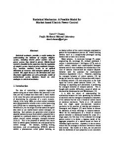
Fig. 3 Learning time dependence of overlap between teacher and student.
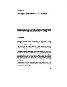
Fig. 2 Learning time dependence of the student length.
=
ησ 2 M (M + 2)(M + 4) 8(2 − (M + 2)η)
ησ 2 M (M + 2)(M + 4) −η(2−(M +2)η)t (0) e + εg − . 8(2 − (M + 2)η)
(31)
From Eqs. (31) and (29), we therefore show that (l(t) )2 becomes larger due to cross-talk noise from other outputs, and so the generalization error worsens as output number M increases. Moreover, the convergence condition of NP-learning of 0 < η < 2/(M + 2) is given by Eq. (31). This condition can be rewritten as 2(1 − η) . (32) M< η Consequently, we calculate the asymptotic value of the generalization error by substituting t → ∞ into Eq. (31). ησ 2 M (M + 2)(M + 4) ε(∞) . (33) = g (8(2 − (M + 2)η) The asymptotic value of the generalization error is vanished in the limit η → 0. Next, we compare the analytical results with those of computer simulation to examine the validity of analysis. We show results for the student length (l(t) )2 (t) (Fig. 2), the overlap r(t) = R(t) l(t) (Fig. 3) and the generalization error εg (Fig. 4). We set the output unit number M = 2, 5, or 8; set the standard deviation σ = 0.2; and set the learning rate η = 0.1. The results were obtained
IPSJ Transactions on Mathematical Modeling and Its Applications
Vol. 4
No. 1
Fig. 4 Learning time dependence of the generalization error.
through computer simulation with N = 1,000 and each point obtained through averaging over 50 trials. Each element of the teacher and initial student weight vectors was independently drawn from the distribution of N (0, 1), and the element of input is drawn from N (0, 1/N ). In the figures, the theoretical results for M = 2 are shown by a dotted line, the results for M = 5 are shown by a dashed line, and the results for M = 8 are shown by a solid line. The simulation results for M = 2 are represented by “+ ×”, those for M = 5 by “×”, and those for M = 8 by “+”. The horizontal axis of each figure is normalized time t = m/N , where
72–81 (Jan. 2011)
c 2011 Information Processing Society of Japan �
78
Statistical Mechanics of On-line Node-perturbation Learning
m is the number of learning iterations. Figure 2 shows the learning time dependence for student length l2 . The vertical axis is the student length. As shown, the analytical results agreed with those of the computer simulations, confirming the validity of the theoretical assumptions. The student length becomes longer as the output number M increases, and this result supports the analytical observations. Figure 3 shows the time dependence of overlap between the teacher and student r = Rl. The vertical axis is the overlap r. As shown, the analytical results again agreed with those of the computer simulations. Moreover, the overlap between teacher and student does not depend on output number M , and this supports the analytical observations. Figure 4 shows time dependence of the generalization error. The vertical axis is the generalization error εg . As shown, analytical results agreed with those of the computer simulations. The generalization error becomes larger as the output number M increases, and this phenomenon is due to the M dependence of l2 . This result supports the analytical observations. The above results show the validity of the analytical solutions. 5. Discussion In the present paper, we derived the generalization error by using a statistical mechanics method. On the other hand, Werfel, et al. 3) derived the discrete evolution equation of the squared error as a learning curve by averaging the squared error over the possible inputs. These two methods use different techniques, so it is useful to clarify the relation between the methods. For comparison, we re-formulate Werfel’s formulation of the norm of the in√ put ||x|| as O(1), while it was originally formulated as O( N ), and re-derive Werfel’s learning curve by following their analysis. (The derivation is shown in the Appendix.) � � ησ 2 (M + 2)(M + 4)M E (m) = 8 (2 − (M + 2)η) � � m ησ 2 (M + 2)(M + 4)M (0) + E − (34) e−η(2−η(N +2)) N . 8 (2 − (M + 2)η) (0) If we substitute t = m/N and E (0) = εg , Eq. (34) becomes identical to Eq. (31).
IPSJ Transactions on Mathematical Modeling and Its Applications
Vol. 4
No. 1
Next, we compare results obtained through the statistical mechanics method with those of Werfel, et al. 3) . From the statistical mechanics results, Eq. (29) shows that cross-talk noise is the cause of the longer student length as output number M increases. Equation (28) shows that the overlap r remains constant when output number M changes. Therefore, as we have shown, when the output number M becomes larger, the cross-talk noise from other outputs will increase the student vector length and the generalization error will become larger. Our result describes the deterministic behavior of the system while Werfel’s result is just an average of the squared error. Moreover, statistical mechanical analysis can treat the case of nonlinear output functions through statistical mechanical methods while Werfel’s analysis method cannot. On the other hand, when the input number is finite, we cannot analyze the system because we assume an infinite number N in the statistical mechanical method. The previous study 3) also showed that the generalization error becomes larger for a larger output number M , and their approach enables analysis of the case of finite input number N . However, it cannot show the cause of the larger generalization error for a larger output number M . The previous studies cannot analyze the case using nonlinear output functions. 6. Conclusion We have analyzed node perturbation learning (NP-learning) using a statistical mechanical method within the framework of on-line learning. NP-learning is a kind of stochastic gradient method and it can be widely used in machine learning. We formulated NP-learning by using the teacher-student formulation, and we assumed the thermodynamic limit of N → ∞. We showed that NPlearning can be formulated as noisy perceptron learning, and then derived the differential equations of order parameters that depict the learning process. The order parameters of NP-learning are the length of the student weight vector lk and the overlap between teacher and student Rk . We derived these differential equations using a statistical mechanics method and solved them analytically. We then derived dynamics of the generalization error using these order parameters. Consequently, we showed that when the output number M becomes larger, the cross-talk noise from other outputs increases the student vector length and the
72–81 (Jan. 2011)
c 2011 Information Processing Society of Japan �
79
Statistical Mechanics of On-line Node-perturbation Learning
generalization error becomes larger. We also showed that the effect of cross-talk noise for larger number of outputs can be canceled out by decreasing the learning rate η. Our future work will include the analysis of NP-learning with a non-linear output function. References 1) Widrow, B. and Lehr, M.A.: 30 years of adaptive neural networks: Perceptron, Madaline, and Backpropagation, Proc. IEEE, Vol.78, No.9, pp.1415–1442 (1990). 2) Williams, R.J.: Simple Statistical Gradient-Following Algorithms for Connectionist Reinforcement Learning, Machine Learning, Vol.8, pp.229–256 (1992). 3) Werfel, J., Xie, X. and Seung, H.S.: Learning Curves for Stochastic Gradient Descent in Linear Feedforward Networks, Neural Computation, Vol.17, pp.2699–2718 (2005). 4) Sprekeler, H., Hennequin, G. and Gerstner, W.: Code-specific policy gradient rules for spiking neurons, Proc. Neural Information Processing Systems 2010, The MIT press, pp.19–28 (2010). 5) Fiete, I.R. and Seung, H.S.: Gradient Learning in Spiking Neural Networks by Dynamic Perturbation of Conductances, Physical Review Letters, Vol.97, p.048104 (2006). 6) Fiete, I.R., Fee, M.S. and Seung, H.S.: Model of Birdsong Learning Based on Gradient Estimation by Dynamic Perturbation of Neural Conductances, Journal of Neurophysiology, Vol.98, pp.2038–2057 (2007). 7) Reents, G. and Urbanczik, R.: Self-Averaging and On-line Learning, Physical Review Letters, Vol.80, pp.5445–5448 (1998). 8) Biehl, M. and Riegler, P.: On-Line Learning with a Perceptron, Europhysics Letters, Vol.28, No.7, pp.525–530 (1994). 9) Engel, A. and den Broeck, C.V.: Statistical Mechanics of Learning, Cambridge University Press, Cambridge, UK, 1st edition (2001). 10) Hara, K. and Okada, M.: Ensemble Learning of Linear Perceptrons: On-Line Learning Theory, Journal of the Physical Society of Japan, Vol.74, No.11, pp.2966– 2972 (2005). 11) Nishimori, H.: Spin Glass Theory and Statistical Mechanics of Information, Oxford University Press, Oxford, UK (2001). 12) Saad, D.: On-Line Learning in Neural Networks, Cambridge University Press, Cambridge, UK (1992). 13) Krogh, A.: Learning with noise in a linear perceptron, Journal of Physics A: Mathematical and General, Vol.25, No.5, pp.1119–1133 (1992). 14) Krogh, A. and Hertz, J.A.: Generalization on a linear perceptron in the presence of noise, Journal of Physics A: Mathematical and General, Vol.25, No.5, pp.1135–1147 (1992).
IPSJ Transactions on Mathematical Modeling and Its Applications
Vol. 4
No. 1
Appendix A.1 Analysis of Linear Perceptron Learning with Noise In linear perceptron learning with noise, noise ξ (m) is added on the teacher output or student output in the learning process. The learning equation is w(m+1) = w(m) + η(d(m) − y (m) − ξ (m) )x(m) = w(m) + ηf (m) x(m) .
(35)
Here, the noise ξ m is drawn from N (0, σ 2 ). First, we derive the differential equation of student length l. We can rewrite Eq. (6) as w · w = N lk2 , and we square both sides of Eq. (35). N (l(m+1) )2 = N (l(m) )2 + 2ηf (m) y (m) + η 2 (f (m) )2 .
(36)
Note that x and w are random variables, so the equation becomes a random recurrence formula. We formulate the size of input ||x|| as O(1) and the size of √ student weight vector ||w|| as O( N ), so the length of the weight vector has a self-averaging property. Equation (36) is then rewritten as � � N (l(m+1) )2 = N (l(m) )2 + 2η �f y� + η 2 f 2 . (37) Here, �·� denotes the average over possible inputs. Next, we rewrite m as m = N t, and represent the learning process using continuous time t in the thermodynamic limit of N → ∞. At the limit, Eq. (37) becomes a differential equation, so we put l(m) → l, l(m+1) → l + dlk , 1/N → dt, and then obtain the deterministic differential equation of lk : � � 2 N (l + dl) = N l2 + 2η �f y� + η 2 f 2 , � � dl2 = 2η �f y� + η 2 f 2 . (38) dt Here, time t is omitted from functions l, y, and f for the sake of simplicity. Next, we derive the differential equation of R that is the second order parameter of the system. R is the direction cosine (overlap) between teacher weight vector w∗ and student weigh vector w defined as w∗ · w w∗ · w R≡ = . (39) ||w∗ ||||w|| Nl The differential equation of overlap R is derived by calculating the product of w∗
72–81 (Jan. 2011)
c 2011 Information Processing Society of Japan �
80
Statistical Mechanics of On-line Node-perturbation Learning
and Eq. (35), and we then obtain the term of the equation using the distribution of P (d, y). We then get N r(m+1) = N r(m) + η �f d� .
(40)
Here, we write overlap between the teacher weight vector and the student weight vector as r and r = Rl for the sake of convenience. The overlap R also has a self-averaging in the thermodynamic limit, and the deterministic differential equation of r is then obtained through a calculation similar to that used for l. dr = η �f d� . (41) dt Here, time t is omitted from functions r, d, and f for the sake of simplicity. �·� denote the average over the possible inputs. The three averages in Eqs. (38) and (41) are calculated as � � �f · y� = �(d − y − ξ)y� = �dy� − (y)2 − �ξy� = r − l2 , (42) � � 2� � 2 f = (d − y − ξ) � � � � � � = (d)2 + (y)2 + (ξ)2 − 2 �dy� + 2 �yξ� − 2 �dξ� = 1 − 2r + l2 + σ 2 ,
�
2
�f · d� = �(d − y − ξ)d� = (d)
�
(43) − �yd� − �ξd� = 1 − r.
(44)
As a result, differential equations of the order parameters are give as dl = 2η(r − l2 ) + η 2 (1 − 2r + l2 + σ 2 ), dt dr = η(1 − r). dt
(45) (46)
A.2 Derivation of Learning Curve of NP-learning To compare statistical mechanics results with that of Werfel’s, we change the √ formulation of norm of input ||x|| from O( N ) to O(1), and derive the learning curve of NP-learning by following the derivation of Werfel, et al. 3) . We rewrite Eq. (7) as 1 1 1 (47) E = ||d − y||2 = ||(w∗ − w) · x||2 = ||W · x||2 . 2 2 2 The learning curve shows the behavior of the squared error between the teacher
IPSJ Transactions on Mathematical Modeling and Its Applications
Vol. 4
No. 1
outputs and those of the students. We calculate an ensemble of averages of the squared error �E� by expanding Eq. (7). �N M
2 � � 1� � 1 � � � (m) (m) (m) (m) (m) 2 = ||W · x || = Wik xk E 2 2 i=1 k=1 ⎡� � �M �⎤ N M � � (m) �2 � (m) �2 1 � ⎣ � (m) m � (m) (m) ⎦ = Wik xk Win xn + Wik xk 2 i=1 k=1
=
1 2
N � M �� � i=1 k=1
n�=k
�2 � 1 (m) Wik . N
k=1
(48)
Here, we assume that an input element xi is drawn from a probabilistic distribution with zero mean and N1 variance. To calculate Eq. (48), we need to obtain the time evolution of the ensemble average of the square of student weight vector � � �2 � (m) (1) Wik . The square of the weight vector of one-step update Wik is given by Eq. (9) as follows; �2 � �2 � � �2 � η � (0) (1) (0) (0) (0) (0) (0) Wij = Wij + ΔWij = Wij − 2 EN P − E (0) ξi xj . σ (49) By substituting Eqs. (7) and (8) into Eq. (49) and then averaging the term over the possible input, we get � � �� � �2 � �� �2 � � 2η η 2 � (0) �2 (1) (0) Wij Wij Wij = 1− (M N + 2N + 2M + 4) + 2 N N η2 σ2 (M + 2)(M + 4). (50) + 4N� � � � � � � � � � Here, we have used x2i = 1/N , ξ 2 = σ 2 , ξ 4 = 3σ 4 , ξ 6 = 15σ 6 , ξ 3 = � 5� ξ = 0. Applying Eq. (50) for the m-th iteration, summing up for i and j, and then substituting them into Eq. (48), we get the learning equation as � ησ 2 (M + 2)(M + 4)M � E (t) = 8 (2 − (M + 2)η) � � ησ 2 (M + 2)(M + 4)M + E (0) − (51) e−η(2−η(N +2))t . 8 (2 − (M + 2)η)
72–81 (Jan. 2011)
c 2011 Information Processing Society of Japan �
81
Statistical Mechanics of On-line Node-perturbation Learning
Here, time t is defined as t = m/N , and the ensemble average of the squared � � error at t is E (t) , and that of the squared error at t = 0 is E (0) . (Received August 27, 2010) (Revised October 9, 2010) (Accepted October 22, 2010) Kazuyuki Hara received his B.Eng. and M.Eng. degrees from Nihon University in 1979 and 1981 respectively and Ph.D. degree from Kanazawa University in 1997. He was involved in NEC Home Electronics Corporation from 1981 until 1987. He joined to Toyama Polytechnic College in 1987 where he was a lecturer. He joined Tokyo Metropolitan College of Technology in 1998 where he was an associate professor and became a professor in 2005. He became a professor at Nihon University in 2010. His current research interests include statistical mechanics of on-line learning. Kentaro Katahira received his B.S. degree from Chiba University in 2002 and M.S. and Ph.D. degrees from The University of Tokyo in 2004, 2009, respectively. From 2004 to 2005, he worked at Yamaha Corporation. Currently, he is an researcher of Japan Science Technology Agency, ERATO, OKANOYA Emotional Information Project. His research interests include statistical data modeling, decision making and statistical learning.
IPSJ Transactions on Mathematical Modeling and Its Applications
Vol. 4
No. 1
Kazuo Okanoya received the B.S. degree from Keio University in 1983. He received his M.S. and Ph.D. degrees from University of Maryland in 1986 and 1989, respectively. From 1989 to 1990, he was a post-doctoral fellow of JSPS. From 1990 to 1993, he was a post-doctoral fellow of JST. From 1994 to 2005, he was an associate professor at Department of Cognitive and Information Sciences, Faculty of Letters, Chiba University. Currently, he is a laboratory head of laboratory for Biolinguistics, RIKEN Brain Science Institute, a research director of OKANOYA Emotional Information Project, JST ERATO, and a professor of Graduate School of Arts and Sciences, The University of Tokyo. His research interest is in biological inquiry into the origin of language and emotion. Masato Okada received his B.Sc. degree in physics from Osaka City University in 1985, M.Sc. degree in physics and Ph.D. degree in science from Osaka University, Osaka, Japan, in 1987, and 1997, respectively. From 1987 to 1989, he worked at Mitsubishi Electric Corporation, and from 1991 to 1996, he was a research associate at Osaka University. He was a researcher on the Kawato Dynamic Brain Project until 2001. He was a deputy head of the Laboratory for Mathematical Neuroscience, RIKEN Brain Science Institute, Saitama, Japan, and a PRESTO researcher on intelligent cooperation and control at the Japan Science and Technology Agency until 2004. Currently, he is a professor in the Graduate School of Frontier Science, The University of Tokyo. His research interests include the computational aspects of neural networks and statistical mechanics for information processing.
72–81 (Jan. 2011)
c 2011 Information Processing Society of Japan �