Statistical Models for Hardened Properties of Self-Compacting Concrete

American J. of Engineering and Applied Sciences 2 (4): 764-770, 2009 ISSN 1941-7020 © 2009 Science Publications

Statistical Models for Hardened Properties of Self-Compacting Concrete 1

Arabi N.S. Al Qadi, 1Kamal Nasharuddin Bin Mustapha, 2 Hashem Al-Mattarneh and 3Qahir N.S. AL-Kadi 1 Department of Civil Engineering, University Tenaga National, Malaysia 2 Faculty of Engineering, Jerash Private University, Jordan 3 The Hashemite University, Zarqa, Jordan Abstract: Problem statement: For predicting workability and hardened properties of SelfCompacting Concrete (SCC) no well known explicit formulation. Approach: Statistical models were carried out to model the influence of key mixture parameter (cement, water to powder ratio, fly ash and super plasticizer) on hardened properties affecting the performance of SCC. Such responses included compressive strength at 3, 7 and 28 days and modulus of elasticity. Thirty one mixtures were prepared to derive the numerical models and evaluate the accuracy. The models were valid for a wide range of mixture proportioning. Results: The research presented derived numerical models that can be useful to reduce the test procedures and trials needed for the proportioning of self-compacting concrete. The qualities of these models were evaluated based on several factors such as level prediction, residual error, residual mean square and correlation coefficients. Conclusion: Full quadratic models in all the response (compressive strength at 3,7 and 28 days and modulus of elasticity) showed high correlation coefficient (R2), adjusted correlation coefficient, less level of significant and sum of square errors from the four predictions models (linear, interaction, full quadratic and pure quadratic) were developed. Key words: Hardened SCC, central composite, self-compacting concrete ultrasonic velocity (uv), absorption and shrinkage. He conclude that a high strength and low shrinkage by the increasing the content of fly ash a 40% replacement of cement gave 65 N mm−1 2 at 56 days, but the high absorption was happen by the increase of fly ash contents a 2% absorption was shown. Also, there is a reduction in shrinkage by the increase of fly ash content. A linear relation ship was happen between fly ash content with 56 days shrinkage and a sharp decrease relation between absorption and strength by increasing absorption 1-2%. Mehta[3] the static modulus of elasticity of a material under tension or compression is given by the slope of the stress (σ) -strain (ε) curve under uniaxial loading. Three methods for calculating the modulus are used for concrete such as initial tangent modulus, secant modulus and chord modulus. Vengala[4] found that use of fine fly ash for obtaining Self Compacting Concrete resulted in an increase of the 28 day Compressive Strength Concrete by about 38%. Self Compacting Concrete was achieved when volume of paste was between 0.43 and 0.45. Tests for compressive strength at 3, 7 and 28 days and modulus of elasticity were conducted using Universal Testing Machine (UTM) 1000 KN.

INTRODUCTION The mechanical properties and behavior of SCC are similar to conventional concrete in terms of compressive strength. There is some concern that SCC may have a lower modulus of elasticity due to lower coarse aggregate content, which may affect deformation characteristics of pre-stressed concrete members. Additionally, creep and shrinkage are expected to be higher for SCC due to its high paste content, affecting pre-stress loss and long term deflection, although this may be offset in part due to relatively low w/c of SCC commonly used in pre-cast operations. Previous research: Frank et al.[1] Verify the mechanical properties of SCC before using it for practical applications, the time development of the material properties and the bond behavior between the reinforcing bars and the SCC as basis for the description of the load bearing capacity of reinforced concrete structures. Khatib[2] Study the effect of fly-ash on the properties of SCC by replacement the cement content with 0-80% fly-ash. Fixing the water/binder to 0.36 for all mixes. Testing workability, compressive strength,

Corresponding Author: Arabi N.S. Al Qadi, Department of Civil Engineering, University Tenaga National, Malaysia

764

Am. J. Engg. & Applied Sci., 2 (4): 764-770, 2009 and the remaining water were introduced and the concrete was mixed for 3 min. Nine 100×100×100 mm cubic were cast and moist for each mix to determine compressive strength after 3, 7 and 28 days and 3 cylinder 150×300 mm for modulus of elasticity.

MATERIALS AND METHODS Materials properties: The materials that implemented in the research are: Cement: Ordinary Portland cement of available in local market is used in the investigation. The Cement used has been tested for various proportions as per (ASTM C150-85A)[5] the specific gravity was 3.15 and fineness was 2091 cm2 gm−1.

Statistical design of experiment approach: Many researchers have used Design Of Experiment (DOE) techniques to evaluate mix-proportioning effect by selecting trial and optimize proportions. These DOE techniques provide a method to evaluate the effect of different parameters in statically sound manner and with minimum mixture numbers. Models of regression are fitted to the result to each measured response results. A central composite response surface is commonly used approach. Knowledge a bout the materials and proportioning of SCC is required to select the parameters that can be used in the design of experiment and satisfies the SCC characteristics.

Coarse and fine aggregate: Coarse aggregate: Crushed angular granite material of 20 mm max size from a local source was used as course aggregate. The specific gravity of 2.45, absorption value was 1.5%, fineness modulus 6.05 and bulk density of 1480 kg m−3 confirms to ASTM C 33-86[6] was used. The fine aggregates consisted of river sand with maximum size of 4.75 mm, with a modulus of fineness Mx = 4.16; normal grading. Specific gravity was 2.33 and absorption value was 6.4%.

Development of statistical models: Statistical experimental design of four factors at two levels was used to evaluate the influence of two different levels for each variable on the relevant concrete properties. Such two-level factorial design requires a minimum number of tests for each variable[10]. The fact that the expected responses do not vary in a linear manner with the selected variable and to enable the quantification of the prediction of the responses, a central composite plan was selected, where the response could be modeled in a quadratic manner. Since the error in predicting the responses increases with the distance from the centre of the modeled region, it is advisable to limit the use of the models to an area bound by values corresponding to -α to +α limits. The parameters were carefully selected to carry out composite factorial design, where the effect of each factor is evaluated at five different levels, in codified values of -α,-1, 0, 1, +α. The value of α value is chosen so that the variance of the response predict by the model would depend only on the distance from the centre of the modeled region. The value of α value is taken here as ±2. Seven replicate central points were prepared to estimate the degree of experimental error for the modeled responses. Appropriate MiTab software was used for statistical analysis of the results[11]. Four key parameters that can have significant influence on the mix characteristics of SCC were selected to derive the mathematical models for evaluating relevant properties. The experimental levels of the variables (maximum and minimum), boundary of cement content, W/P, fly ash content, Sp dosage are defined.

Fly Ashes (FA): Type-II fly ash from Kapar Thermal Power Station, Selangor, Malaysia, was used as cement replacement material. Fly Ash for use as Pozzolana and Admixture. Class F fly ash was obtained had a specific gravity of 2.323 and fineness of 2423 cm2 g−1 determined as confirms to (ASTM C 618)[7]. Super Plasticizer (SP): Polycarboxylicether (PCE) based super-plasticizer which is Brown Color and free flowing liquid and having Relative density 1.15 Super Plasticizer confirms to ASTM C 494-92[8]. Type A and Type F in aqueous form to enhance workability and water retention. A sulfonated, naphthaleneformaldehyde super plasticizer and a synthetic resin type Air-Entraining Admixture (AEA) were used in all the concrete mixtures. Mixing water: Potable water confirms to ASTM D 1129[9] for mixing the concrete and curing of the reaction. Methods: All concrete mixes were prepared in 40 L batches in a rotating planetary mixer. The batching sequence consisted of homogenizing the sand and coarse aggregate for 30 sec, then adding about half of the mixing water into the mixer and continuing to mix for one more minute. The mixer was covered with plastic cover to minimize the evaporation of the mixing water and to let the dry aggregates in the mixer absorb the water. After 5 min, the cement and fly ash were added and mixed for another minute. Finally, the SP 765

Am. J. Engg. & Applied Sci., 2 (4): 764-770, 2009 DISCUSSION

The modeled experimental region consisted of mixes ranging between the coded variables of -2 to +2 and is given in Table 1. The derived statistical models are valid for mixes with W/P ranging from 0.3-0.38 by mass, dosages of SP ranging from 7.2-10.8 kg m−3 1.8% of total powder content(by mass)[12], cement content ranging from 400-450 kg m−3. The mass of coarse aggregate was 25-35% by volume of the mix. The SCC responses modeled were compressive strengths at 3, 7 and 28 days and modulus of elasticity [13].

Derived models: The mix proportions and test result of 31 mixes prepared to derive the central composite surface design models are summarized in Table 2 and 3, respectively. The result of the derived models in this research is prepared, along with the correlation coefficients and the relative significance, are in Table 3. The estimates for each parameter refer to the coefficients of the model found by a least-square method. The significant of each variable on a given response is evaluated using t test values based on Student’s distribution. Probabilities less than 0.05 are often considered as significant evidence that the parameters are not equal to zero; contribution of the proposed parameter has a highly significant influence on the measured response. The R2 values of the response surface models for the compressive strength 3,

RESULTS Compressive strength is mostly considered as important property of concrete, therefore, the W/P, which affects compressive strength, was chosen to attain the desired strength. In order to achieve high strength, the w/p must be low. SCC has shown an increase in compressive strength, the values used in Table 2 for the variation of compressive strength with w/p ratio. The strength over 41 obtained for 0.3 and 0.38 water-powder ratios. Relation between modulus of elasticity and compressive strengths.

Table 1: Value of coded variables Coded values -2 -1 Cement (kg m−3) 400.0 412.50 W/P ratio 0.3 0.32 FA (kg m−3) 110.0 120.00 SP (kg m−3) 7.2 8.10

Table 2: Mix proportions and properties of hardened SCC of all mixes used in the central composite design X4 X1 X2 X3 ----------------------------------------------Y9 No. Cement (kg m−3) W/P (ratio) FA (kg m−3) SP (kg m−3) Sand (kg m−3) CA (kg m−3) fC3(Mpa) 1 425.0 0.38 130 9.0 861 693 19.876 2 450.0 0.34 130 9.0 869 700 25.877 3 412.5 0.36 120 9.9 898 723 16.739 4 437.5 0.32 140 9.9 884 712 22.829 5 437.5 0.36 120 8.1 877 706 23.520 6 412.5 0.32 140 8.1 909 731 24.564 7 425.0 0.34 130 9.0 892 718 9.7250 8 425.0 0.34 130 9.0 892 718 11.900 9 425.0 0.34 130 9.0 892 718 12.230 10 425.0 0.34 150 9.0 870 701 27.366 11 437.5 0.32 140 8.1 887 714 29.103 12 437.5 0.32 120 9.9 905 728 24.250 13 437.5 0.36 120 9.9 874 704 22.340 14 437.5 0.32 120 8.1 907 730 27.075 15 437.5 0.36 140 9.9 853 686 20.324 16 412.5 0.36 140 8.1 878 707 19.688 17 425.0 0.34 110 9.0 913 735 10.679 18 412.5 0.36 140 9.9 876 705 14.639 19 425.0 0.34 130 9.0 892 718 12.906 20 412.5 0.36 120 8.1 900 725 11.637 21 437.5 0.36 140 8.1 855 688 21.672 22 425.0 0.30 130 9.0 922 742 23.456 23 425.0 0.34 130 7.2 894 720 23.760 24 412.5 0.32 140 9.9 906 729 21.192 25 425.0 0.34 130 9.0 892 718 9.9200 26 425.0 0.34 130 9.0 892 718 10.832 27 425.0 0.34 130 9.0 892 718 11.300 28 425.0 0.34 130 10.8 889 716 16.896 29 412.5 0.32 120 8.1 929 748 17.778 30 412.5 0.32 120 9.9 927 746 9.1360 31 400.0 0.34 130 9.0 914 736 10.745

766

0 425.00 0.34 130.00 9.00

Y10 fC7(Mpa) 27.593 32.534 25.768 29.590 31.800 33.973 35.058 29.050 30.200 36.939 30.059 32.895 29.678 37.814 28.978 27.262 30.116 33.472 28.359 28.648 30.583 33.795 31.843 31.017 32.237 34.051 31.000 30.013 26.494 23.958 22.050

1 437.50 0.36 140.00 9.90

Y11 fC28(Mpa) 35.254 47.095 36.235 46.484 44.307 45.216 48.975 44.543 45.102 48.174 47.181 41.927 39.152 45.997 37.573 40.747 38.587 44.732 43.337 37.051 41.055 42.657 42.433 40.734 46.833 47.752 46.200 41.056 41.451 38.457 35.995

2 450.00 0.38 150.00 10.80

Y12 E (Gpa) 27.890 32.862 31.950 34.926 37.865 38.943 37.494 32.752 30.473 32.096 28.886 32.320 33.798 30.589 31.576 36.931 34.138 38.401 29.939 39.026 30.742 34.345 29.284 31.288 36.234 34.789 33.716 27.214 29.815 38.457 35.995

Am. J. Engg. & Applied Sci., 2 (4): 764-770, 2009 Table 3: Statistical models of compressive strength at 3, 7 and 28 days and modulus of elasticity summary Model R2 (%) R2 AdJ. (%) F-value P-value Resid. lower SSE Residupp. Regression equation Linear fC28 (Mpa) fC7 (Mpa) fC3 (Mpa) E (Gpa) Interaction fC28 (Mpa)

46.6 33.5 45.7 11.7

38.30 23.20 37.30 0.00

5.66 3.27 5.47 0.86

0.002 0.027 0.002 0.501

-4.043 -4.661 -8.467 -5.813

253.000 241.621 637.420 309.620

5.097 5.313 5.763 5.228

Y11 = 1.3+0.138×1-86.3×2+0.160×3- 0.947×4 Y10 = -18.5+0.139×1-45.9×2+0.0897×3-0.692×4 Y9 = - 94.8+0.287×1- 67.8×2+0.229×3-1.73×4 Y12 = 80.0-0.101×1+4.5×2-0.0259×3-0.195×4

55.4

33.10

2.49

0.040

-4.062

211.580

6.320

fC7 (Mpa)

60.5

40.80

3.06

0.016 h

-5.012

143.420

4.602

fC3 (Mpa)

53.9

30.80

2.34

0.051

-8.467

541.320

5.982

E (Gpa)

23.7

0.00

0.62

0.778

-5.813

267.410

4.830

Y11 = -1040+2.77 ×1+1200×2+3.79×3+5.0×43.10×1×2- 0.00866×1×3- 0.0505×1×4 -1.38×2×3 +23.5 ×2×4 + 0.0580 ×3×4 Y10 = -1192+3.45×1+548×2+6.33×3-9.0×42.26×1×2- 0.0169×1×3-0.0386×1×4+0.29×2×3 +36.4×2×4+0.0947×3×4 Y9 = -1170+2.56×1+632×2+8.57×3-16.8×41.36×1×2 -0.0140×1×3+0.002×1×4 -5.43×2×3+ 64.7×2×4 -0.059×3×4 Y12 = -436+0.45×1+931×2+3.85×3-2.4×40.14×1×2 -0.00738×1×3+0.0509×1×4 -2.45×2×3 - 61.1×2×4+0.010×3×4

Full quad. fC28 (Mpa)

82.3

66.90

5.33

0.001

-3.055

83.7950

2.869

fC7 (Mpa)

73.2

49.80

3.13

0.016

-3.034

97.1700

3.636

fC3 (Mpa)

92.0

85.00

13.19

0.000

-4.150

93.5590

3.306

E (Gpa)

36.3

0.00

0.65

0.788

-4.985

223.45

5.290

Pure quad. fC28(Mpa)

73.5

63.80

7.62

0.000

-4.813

125.808

1.649

fC7(Mpa)

46.2

26.60

2.36

0.053

-4.404

195.371

5.569

fC3(Mpa)

83.8

78.00

14.26

0.000

-4.150

189.650

5.306

E (Gpa)

24.2

0.00

0.88

0.549

-4.985

265.660

4.544

7 and 28 day fc and modulus of elasticity are 92, 73.2, 82.3 and 36.3% in full quadratic equation with respect to the linear, interaction and pure quadratic. The high correlation coefficient of the response shows good correlations that considered at least 95% of the measured values can be accounted for proposed models. The accuracy of the proposed models was determined by comparing predicted to measured values

Y11 = - 2992+8.65 ×1+4136×2+5.40×3+27.9×4 - 3.10 ×1×2 -0.00866 ×1×3 -0.0505×1×4-1.38 ×2×3+23.5×2×4+0.0580×3×4 - 0.00691×1×1 4318 ×2×2-0.00621×3×3-1.27×4×4 Y10 = -2500+9.51×1+995×2+5.17×3-4.4×42.26×1×2-0.0169×1×3- 0.0386 ×1×4+0.29×2×3 + 36.4×2×4+0.0947×3×4-0.00713×1×1-658 ×2×2+0.00445×3×3-0.253×4×4 Y9 = 2332-7.56×1-3953×2+3.27×3-69.4 41.36×1×2-0.0140×1×3+0.0019×1×4 -5.43×2×3 + 64.7×2×4 -0.0590×3×4+0.0119×1×1+6743 ×2×2+ 0.0204×3×3+2.92×4×4 Y12 = 134-2.79×1+1328×2+3.16×3+18.8×40.14×1×2-0.00738×1×3+0.0509×1×4 -2.45×2×3 - 61.1×2×4+0.010×3×4+0.00380×1×1-583 ×2×2+0.00267×3×3-1.17×4×4 Y11 = -1951+6.01×1+2850×2+1.77×3+21.9 ×40.00691×1×1 - 4318×2×2-0.00621×3×3-1.27×4×4 Y10 = -1326+6.20×1+401×2-1.07×3+3.9×40.00713×1×1-658×2×2+0.00445×3×3 -0.253×4×4 y9 = 3407- 9.82×1-4653×2-5.07×3-54.2 ×4+ 0.0119×1×1+6743×2×2+0.0204×3×3+2.92×4×4 Y12 = 650-3.34×1+401×2-0.72×3+20.9×4+ 0.00380×1×1-583×2×2+0.00267×3×3-1.17×4×4

The experimental values for compressive strength at 3, 7 and 28 days and modulus of elasticity under different treatment conditions are presented in Table 2. Regression coefficient for polynomial equations and result of linear, interaction, full and pure quadratic are presented in Table 3. Statistical analysis for compressive strength at 28 days indicates that the models with coefficient of correlation R2 for linear, interaction full and pure quadratic are 46.6, 55.4,82.3 and 73.5 Shows that the full quadratic at R2 equal to 82.3 was adequate, possessing less significant lack of fit than other model the better one fit shown in Fig. 1. Moreover, compressive strength at 7 days indicate that the models of R2 = 33.5, 60.5, 73.2 and 46.2 for linear, interaction, full and pure quadratic.

Correlation between measured and predicted models: The response surface methodology was used to investigate the effect of parameters (cement, W/P, FA and SP) on hardened properties (compressive strength at 3,7 and 28 days and modulus of elasticity). The levels of independent parameters were determined based on preliminary experiments as shown in Table 1. 767

Am. J. Engg. & Applied Sci., 2 (4): 764-770, 2009

Fig. 1: Comparison between measured compressive strength at 28 days and predicted values from statistical models

Fig. 3: Comparison between measured compressive strength at 3 days and predicted values from statistical models

Fig. 2: Comparison between measured compressive strength at 7 days and predicted values from statistical models

Fig. 4: Comparison between measured modulus of elasticity and predicted values from statistical models

The closer value to unity is a full quadratic model with R2 = 73.2% is better model fit as shown in Fig. 2. QQ, full and pure quadratic models full quadratic show in Fig. 3 the best fit. Furthermore, modulus of elasticity statistical models with R2 values of the response surface models for linear, interaction, full and pure quadratic models were found to be 11.7, 23.7, 36.3 and 24.2 as shown in Fig. 4 with the best fit is a full quadratic model.

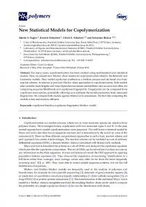
Figure 5 the data of compressive strength at 28 days measured and predicted values of SSE equals to 253,211.58, 83.795 and 125.808 for linear, interaction, full and pure quadratic models indicate that full quadratic less variability of the data point from the line than other models. Therefore, Fig. 6 analyses of data of fc′ at 7 days, SSE equal to 241.621, 143.42.97.17 and 195.371 four the polynomial models indicate that full quadratic is fit than other models. Thus, Fig. 7 the data of fc′ at 3 days the SSE equals to 637.42, 541.32, 93.559 and 189.65 indicate the best is at full quadratic model. Result of Fig. 8 for modulus of elasticity indicate that SSE = 309.62, 267.41, 223.45 and 265.66 the full quadratic is the best one.

Residuals models: Residual is the measure of the deviation of an observed data point from the estimated regression line. If the estimated regression line fits the data points perfectly, error sum of squares (SSE) = 0. The more the line the variability of the data points away from the line, the larger the value for SSE[14]. 768

Am. J. Engg. & Applied Sci., 2 (4): 764-770, 2009

Fig. 5: Residual compressive strength at 28 days for various statistical models

Fig. 8: Residual modulus of elasticity for various statistical models CONCLUSION The effect of the concrete constituents such as cement, water-powder ratio, fly-ash and superplasticizer on hardened properties of self-compacting concrete were investigated based on the result of this research the following conclusions can be drawn: •

• Fig. 6: Residual compressive strength at 7days for various statistical models

•

•

•

A central composite design is a useful tools to evaluate parameters effects of mixture and the interaction between the parameters on SCC that can reduce the number of trials to achieve balance among mix variables Numerical models established for the SCC mixtures can be useful in design of concrete and selecting constituent materials Central composite was selected where the response modeled in a quadratic manner while seven replicate central points were prepared to estimate the degree of experimental error response model Graphical analysis of the residuals shows the deviation between the measured data and the fit one could be effective methods to test the adequacy of the regression model fit Fluctuating of measured residual data in random manner show a satisfactory plot on the band and its clear in full quadratic models for all the sixteen models

Full quadratic models in all the response (compressive strength at 3,7 and 28 days and modulus of elasticity) shows a high correlation coefficient (R2), adjusted correlation coefficient, less level of significant and sum of square errors from the four predictions

Fig. 7: Residual compressive strength at 3 days for various statistical models 769

Am. J. Engg. & Applied Sci., 2 (4): 764-770, 2009 models (linear, interaction, full quadratic and pure quadratic) were developed

6.

ACKNOWLEDGEMENT 7. This research described in this study was conducted at the Civil of Engineering (COE) Department at University Tenaga National (Uniten) at Malaysia and was funded by the Uniten Internal Grant and Ministry of Science, Technology and Innovation (MOSTI), E-Science Grant. (03-02-03-SFO140) also the author would like to thank BASF chemical company for their helps in implementing this research.

8.

9.

10.

REFERENCES 1.

2.

3.

4.

Frank, D., K. Holschemacher and D. Weibe, 2000. Self Compacting Concrete (SCC) time development of the material properties and the bond behavior. LACER no.5. http://www.wilbertprecast.com/documents/scc.pdf Khatib, J.M., 2008. Performance of self compacting concrete containing fly ash. Construct. Build. Mater., 22: 1963-1971. http://www.encyclopedia.com/doc/1G1181225745.html Mehta, P.K. and P.J.M. Monteiro, 1993. Concrete: Structure, Properties and Materials. 2nd Edn., Prentice Hall, ISBN: 0131756214, pp: 548. Jagadish Vengala Sudarsan, M.S. and R.V. Ranganath, 2003. Experimental study for obtaining self-

11.

12.

13.

compacting concrete. Indian Concr. J., 77: 1261-1266.

5.

http://cat.inist.fr/?aModele=afficheN&cpsidt=1541 2276 ASTM Standard C 150, 2006. Specification for Ordinary Portland Cement. Annual Book of ASTM, Standard, Section 04 Construction, Volume 04.02 Concrete and aggregate, ASTM International, 100 BARR HARBOR DRIVE, P O.Box C700,West CONSHOHOCKEN, PA194282959,www.astm.org, year 2006.

14.

770

ASTM C 33-86, 2006. Specification for concrete aggregate. ASTM international. http://www.techstreet.com/cgibin/detail?product_id=1099378,year ASTM C 618, 2006. Specification for coal fly ash and raw or calcined natural pozzolan for use in concrete. ASTM C International. http://www.astm.org/Standards/C618.htm ASTM C 494-92, 2006. Specification for chemical admixture for concrete. ASTM international. http://www.concrete.org/general/fE4-03.pdf ASTM 1129, 2006. Standard terminology relating to water. http://www.astm.info/Standards/D1129.htm Montgomery, D.C., 1996. Design and Analysis of Experiments. 4th Edn., Wily, New York, ISBN: 0444820612, pp: 1229. 1996 MINITAB Handbook, Fourth Edition: A supplementary text that teaches basic statistics using MINITAB, the Handbook features the creative use of plots, application of standard statistical methods to real data, in-depth exploration of data. http:wwwMinitab.com/products/Minitab/14/docum entation.aspx Su, N., K.C. Hsu and H.W. Chai, 2001. A simple mix design method for self compacting concrete. Cement Concr. Res., 31: 1799-1807. http://direct.bl.uk/bld/PlaceOrder.do?UIN=106345 648&ETOC=RN&from=searchengine EFNARC, 2002. Specifications and guideline for self-compacting concrete. UK., pp: 1-32. http://www.efnarc.org/pdf/SandGforSCC.PDF Montgomery, D.C., 2005. Design and Analysis of Experiments. 6th Edn., Arizona State University, John Wily and Sons, Inc., 111 River Street, Hoboken, New Jersey, USA., 07030,(201)7486011,Fax(201)748-6008