Statistical Models for Empirical Component Properties and Assembly-Level Property Predictions: Toward Standard Labeling Gabriel A. Moreno
Scott A. Hissam
Kurt C. Wallnau
Software Engineering Institute Carnegie Mellon University Pittsburgh, PA, USA +1 412-268-4469
Software Engineering Institute Carnegie Mellon University Pittsburgh, PA, USA +1 412-268-6526
Software Engineering Institute Carnegie Mellon University Pittsburgh, PA, USA +1 412-268-3265
[email protected]
[email protected]
[email protected]
ABSTRACT One risk inherent in the use of software components has been that the behavior of assemblies of components is discovered only after their integration. The objective of our work is to enable designers to use known (and certified) component properties as parameters to models that can be used to predict assembly-level properties. Our concern in this paper is with empirical component properties and compositional reasoning, rather than formal properties and reasoning. Empirical component properties must be measured; assessing the effectiveness of predictions based on these properties also involves measurement. This, in turn, introduces systematic and random measurement error. As a consequence, statistical models are needed to describe empirical component properties and predictions. In this position paper, we identify the statistical models that we have found useful in our research, and which we believe can form a basis for standard industry labels for component properties and prediction theories.
Keywords Predictable assembly; Empirical validation; Labeling; Property measurement; Property theory.
1. INTRODUCTION One risk inherent in the use of software components has been that the behavior of assemblies of components is discovered only after their integration. The objective of our work is to enable designers to use known (and certified) component properties as parameters to models that can be used to predict assembly-level properties.
Of course, this objective is not unique to our work. It could, in fact, be considered a fundamental goal of software engineering. In the realm of theoretical computer science, a significant body of research has accumulated under the general heading of compositional reasoning. Compositional reasoning is nothing more than divide and conquer. That is, we translate something that we need to know about the whole (i.e., the assembly) into things we need to know about its parts (i.e., its components)1. It is, presumably, easier to obtain the properties of the parts than that of the whole. Of course, having obtained the properties of the parts we need to combine (or compose) them to achieve the whole; hence, compositional reasoning. Much of the theoretical work on compositional reasoning stems from research in formal systems. In these systems, component properties are specified in a formal logic, for example temporal logic, and are combined using compositional operators in that logic. Formal approaches to compositional reasoning treat software components as mathematical objects that are described by mathematical models, for example labeled transition networks. While the mathematical treatment of software components is the great strength of any formal approach, it is also its Achilles heel. Automated theorem proving is known to be NP-complete, and thus introduce new problems of scale and complexity in place of those eliminated by divide and conquer. We do not argue against formal reasoning. Instead, we observe that where formal approaches are infeasible, empirical approaches must be used. In this setting, software components and component assemblies are treated as physical rather than mathematical objects. Component and assembly properties are observed rather than asserted (or proved); assembly properties are predicted through the use of theories, rather than demonstrated through proofs of theorems. At its limit, the empirical approach is indistin-
1
We set aside the question of whether compositional reasoning in component-based systems can done by bottom-up synthesis rather than top-down analysis. We merely observe that synthesis is desirable where pre-existing components are to be reused in different applications.
guishable from the fabled scientific method. Many practical and theoretical justifications for the use of an empirical approach to compositional reasoning can be found in Herbert Simon’s classic, The Sciences of the Artificial [7]. Rigorous observation in the empirical approach takes the form of measurement. For reasons both obvious and arcane, measurement invariably introduces error. Thus, empirical component properties are described not as discrete values, but as probability density functions over a range of values. Assessing the effectiveness of a property theory also involves measurement, this time in a more classical application of the scientific method. The property theory is a hypothesis; we attempt to falsify the hypothesis by comparing predicted assembly properties with measured assembly properties. Thus, like component properties, measured assembly properties are described using probability density functions over a range of values. The “scientific” validity of property theories is expressed statistically by both descriptive and inferential methods. We use Figure 1 to introduce and relate terminology used in the remainder of this paper: assemblies (dashed boxes), components (solid boxes), component properties (triangles), programming interfaces (lollipops), control/data composition (‘c1•c2’), and analytic composition via a property theory (‘F’). The property theory is parameterized by a set of component properties (‘Cp’), a set of component interactions (‘Ci’), and environmental factors (‘E’). One premise of our research is that we can suitably constrain the interaction topology and mechanisms, and the environment, to facilitate component property certification and compositional reasoning from certified properties. This applies to both formal and empirical compositional reasoning. This paper is concerned solely with empirical properties and theories.
A
c1.p c1
c2.p c2
p = F(Cp, Ci, E)
c1 • c2
Figure 1. The assembly property (‘A.p’) is computed by function (‘F’). This function expresses a property theory. (‘Cp’) denotes the set of component properties, not necessarily of the same domain, (‘Ci’) the set of enabled interactions, here simply (‘c1 • c2’), and (‘E’) the set of environmental factors.
Our position is that all empirical properties and property theories can be described in a uniform way, using the same, or very similar, statistical models. A fundamental statistical model for measures of component property and assessments of the effectiveness of property theories is the statistical interval (Sect. 2.). Statistical intervals can be used to describe component properties (Sect. 3.) and property theories (Sect. 4.). The use of statistical intervals to describe component properties and property theories presents several new challenges that must be addressed, including uniform treatment of measurement error, propagation of error, and descriptions of the sample set of assemblies against which property theories are vali-
dated1 (Sect. 5.). We conclude with conjectures about desirable characteristics of standard labels beyond particular statistical models (Sect. 6.).
2. STATISTICAL INTERVALS It is said that the “Eskimo” have dozens of words for snow2. While this might be a matter of interpretation, personal experience suggests that statisticians have a different kind of statistical interval for every occasion. We limit our discussion to only the most rudimentary aspects of intervals; interested readers might consult standard texts for more detailed information [4, 9]. Intervals have two uses in our context. One use is to express the estimated value of component properties, and the quality of these estimates. A second use of intervals is inferential: to predict the future performance of components and property theories. Within this second use, we will find it useful to distinguish between normative confidence intervals and an informative3 tolerance intervals. In a normative confidence interval, an interval ± x is specified in measurement units appropriate for a property, and the probability p that the norm will be satisfied by some object is calculated. When used informatively, we do the converse: p is specified, and the interval is calculated. We would use the normative interval if we were interested in what proportion of a population will satisfy stated norms. We would use the informative interval if we wanted to know the interval that contained some proportion of a population. Different statistical intervals apply to different distributions of data. Where data distribution is not normal, it might be transformed into a normal distribution using a standard inversable function defined for this purpose, for example one of the Box-Cox family of transformations, although subtleties attend to the interpretation of the inverted transformation [4]. It might be that the data, while not normal, follows some other distribution, e.g., Weibull, for which there are corresponding methods for calculating intervals. If all else fails, there are distribution-free methods for calculating intervals; although such methods yield wider intervals, they will be sound. Although the ideas we present herein apply to any empirical property, throughout the remainder of this paper we will use latency as the property of interest for components and assemblies. The illustrations are drawn from a small-scale experiment conducted at the SEI [5, 6]; in the text, all references to “our experiment” or similar
1
More accurately, attempt to falsify.
2
See http://www.urbanlegends.com/language/ eskimo_words_for_snow_derby.html
3
Although some readers may prefer the classification prescriptive/descriptive, we opt for using the classification normative/ informative when referring to the purpose of the intervals. It would be statistically incorrect to call a statistical interval descriptive because they all belong to what is called inferential statistics—as opposed to descriptive statistics.
phrases refer to this work. Notationally, c.p denotes property p of component c; analogously, a.p denotes property p of assembly a. Uppercase letters generally denote sets, and lowercase letters denote set elements.
3. COMPONENT LABELS The measurement and subsequent description of empirical component properties does not introduce novel methodological challenges. Objective measurement requires a measurement object (the component), a measurement scale for the component property of interest (e.g., time, in seconds), and a measurement apparatus (e.g., the Microsoft Windows’ high-performance clock). Measurement is conducted with the apparatus within some controlled environment, with control exerted over all independent variables of the dependent (measured) property.
3.1 Fundamental Label: The Property Measurement In general, the measurand Y, or property of interest, is a function of N values: Y = f(X1, X 2, …, X N) [8]. For our latency experiment these values included, in different combinations depending upon component type, execution time, blocking time, and period. We would like to know the true value of Y, component latency. Of course, the true value is not obtainable, as the following definition makes clear:
True Value: the mean (µ) that would result from an infinite number of measurements of the same measurand carried out under repeatability conditions, assuming no systematic error. Because we can not, even in principle, know the true value of µ, we must use an estimator for it, produced by statistical methods. For example, we take a sample of observations of X, and use its average x as the estimator of µ, a population parameter. The uncertainty associated with this estimator is expressed as the standard deviation s such that the true—and unknown—value of µ will fall within some interval x ± ks with some specified confidence. The factor k is known as coverage factor. When k=1, x ± ks yields a 68% confidence interval. That is, we have 0.68 confidence that this interval contains µ. Typically, we compute the 0.95 confidence interval (k=2), which yields higher confidence but a larger bound. This confidence interval expresses a fundamental component measure; it is fundamental because x ± ks is how a component property is modeled in any property theory parameterized by that component property.
3.2 Secondary Labels: Predictions of Future Property Measurements It might be useful to have other descriptors, or labels, for component properties. One such label is the tolerance interval. For example, in the case of component latency, the consumer might want to know what latency interval ± x ms contains a specified proportion p of all executions of component c. For instance, a tolerance interval with p=0.95 might state that there is a 0.95 probability that any
given execution of a component will have a latency of 50ms ± 17ms , where ± 17ms is the computed interval. Another potentially useful label is the conceptual, but not mathematical1, inverse of the above tolerance interval. This is the confidence interval on the probability of satisfying some property specification. It is conceptually the inverse of the tolerance interval since here we specify the latency interval and from this compute the probability that any particular execution will fall within this interval. For example, we might specify the latency interval ± 5ms and from this calculate that there is a 0.64 probability that any given execution of a component will fall within the interval 50ms ± 5 ms . The tolerance interval is useful for informative purposes; it informs the consumer about the likely performance of a component with respect to a property. The confidence interval on the probability of meeting a specification is useful for normative purposes; it informs the consumer about the probability that a component will satisfy a specified norm.
4. PROPERTY THEORY LABELS Measuring and describing the effectiveness of property theories is methodologically more challenging than measuring component properties. As noted earlier, at the limit this measurement process reduces to theory falsification as it is practiced in the empirical sciences; in that sense, at least, no new ground is broken. Our concern is with characterizing (labeling) the quality of a property theory, which translates into labeling the accuracy of its predictions, and how often they are accurate.
4.1 Fundamental Labels: One-Tail Inferential Intervals We again use inferential statistical models to characterize how effective a property theory is likely to be for future predictions. For this purpose we use the confidence and tolerance intervals described in Sect. 3.2. In this case, though, instead of latency, we are interested in the magnitude of relative error (MRE) between predicted and observed latency: a.λ′ – a.λ MRE = -------------------------a.λ where a.λ′ is the measured assembly latency and a.λ is the predicted latency.2 A normative confidence interval will describe the probability that the MRE for a particular prediction will lie within a specified MRE interval.
1
There are different equations used to compute these two forms of intervals.
2
We note in passing that a.λ′ is itself described using the fundamental label used for components. That is, for statistical analysis, the assembly is treated as a component, and the estimator for assembly latency is described by an interval obtained using a coverage factor k=2.
Notice that the lower bounds for an MRE interval represents situations where predictions are better than the mean MRE of the statistical sample (in our experiment, for N=30 assemblies). While we may wish to know how frequently our predictions are better than the mean, we may also only be concerned with the occasions when the predictions are worse than the mean. In this case we use a onetail interval, or bound, instead of a two-tail interval. The one-tail tolerance interval for our experimental latency theory is summarized in Table 1. Table 1. : Tolerance Interval for Property Theory
N = 30
sample size
γ = 0.95
confidence level
p = 0.90
proportion
µMRE = 1.99%
MRE
UB = 6.33 %
upper bound
To compute these results we supplied the sample size N=30, the desired confidence level γ = 0.95, and the proportion of the population p=0.90 we wished to include within the tolerance interval. UB = 0.0633 is the computed upper bound of the tolerance interval. This is interpreted as stating that we have a probability of 0.90 that any particular latency prediction will have an MRE no greater than 6.33%, and we have 0.95 confidence in this upper bound. As with measures of component properties, one and two-tail normative confidence intervals can be computed by specifying interval bounds and computing p, the probability that any particular prediction will satisfy these specified bounds.
to become reality, several important challenges must be addressed. The two discussed here, uncertainty propagation and bounded design space, are not by any means the only challenges, just the ones that present the most immediate obstacles in our research path.
5.1 Uncertainty Propagation All measurement entails error of two sorts: systematic, and random. Systematic error is introduced by the measurement apparatus and measurement process. Code instrumentation for latency imposes execution overhead, and is therefore a source of systematic error. Fluctuation of environmental variables that are not under complete experimental control, for example CPU load introduced by background operating system processes, is one source of random error; the inherent (in)accuracy of measurement instruments is another. Two questions arise: how to express uncertainty of component properties? and, how to propagate this uncertainty through property theories?
Component Property Uncertainty. Recall that the measure of property Y is a function of N values: Y = f(X1, X 2, …, X N) , where at least some of Xi are themselves measurands of the component1. Assuming all Xi are measurands for simplicity, we know that we can at best provide estimators xi of these values, and use them to compute y = f(x 1, x 2, …, x N) , which is an estimator for Y. The combined uncertainty u c(y) is determined by the law of propagation of uncertainty [8]: N 2
u c (y) =
∑ i=1
∂f u 2(x ) + 2 i ∂ x i 2
N–1
N
∑ ∑ i = 1j = i+1
∂f ∂f u(x , x ) ∂ xi ∂ x j i j
4.2 Secondary Labels: Linear Correlation Linear correlation is a descriptive statistic: it describes the strength of correlation between two datasets; it is not directly useful for drawing inferences about future datasets. A consumer might be interested in linear correlation analysis as a descriptor of previous experimental validations of the accuracy of a property theory. We characterize the accuracy of the property theory using correlation analysis. Correlation analysis allows us to assess the strength of the linearly relation between two variables, in our case, predicted and observed assembly latency. The result of this analysis is the coefficient of determination, 0 ≤ R2 ≤ 1, where 0 represents no relation, and 1 represents a perfect linear relation. In a perfect prediction model, predicted and observed latency would be identical; therefore, the goal for the model builder is a linear relation. The property theory we developed as part of our small-scale experiment yielded R2 = 0.9999657, with a significance level α = 0.01. This result means that the property theory accounted for 99.99% of the variation in observed latency; moreover, the significance level means that there is only a 0.01 probability that this correlation could have been achieved by chance.
where
u ( x i, x j ) is the covariance of xi and xj, which is a measure of how strongly correlated the two variables are. To illustrate, our measure of component latency was dependent upon two measurands, X1 for the measured latency of the component, and X2 for the correction2 for the overhead to start and stop the high performance clock (the “stopwatch”); the latter term accounts for the major source of systematic error. The component latency was obtained with the formula Y = X1 + X 2 . We use the above law to compute the standard uncertainty of y. Fortunately, there are simplifications. The second term is 0 because x1 and x2 are un-correlated, so their covariance is 0. In addition, the partial derivatives in the first term are always 1, independently of the value of xi for which they are evaluated.
1
We might, for example, measure component latency as an aggregate of component execution time and component wait time, each of which can be separately measured.
2
The correction for a systematic error is the negative of the measured error.
5. CHALLENGES We have presented several useful statistical models for describing the properties of components and property theories, and for inferring future performance. Nonetheless, for standard empirical labels
∂f ∂f is the partial derivative evaluated in xi, and ∂ xi ∂ Xi
In this case, then, the standard uncertainty of component latency y is u c(y) =
2
2
u (x 1) + u (x 2) . Clearly, the computation is more
unpleasant in situations where the measurands are correlated, for example as might be the case if latency were sensitive to variable heap size and execution duration. Finding all such significant interactions is no trivial matter. Still, making explicit and accommodating measurement uncertainty in the description of empirical component properties is no more onerous than experimental measurement in any empirical science.
Property Theory Uncertainty. In principle, the generality of
Y = f(X1, X 2, …, X N) ought to apply equally to assemblies of components as to components themselves because a predicted assembly property is a function of measured component properties, which are subject to uncertainty. In fact, this formulation is quite consistent with the canonical property theory described in Figure 1: substituting Y for p, and allowing {X1, X2, ..., Xn} = Cp ∪ E, gives us the same formulations, but with one important distinction: the canonical property theory includes a term to denote the patterns of runtime (control and data passing) interaction among components. It is an article of faith in the software architecture research community, perhaps not sufficiently tested by empirical means, that patterns of component interaction will influence assembly properties. In any event, quantifying the impact on assembly properties of patterns of interaction is a significant challenge, although some work has been done in this area [1]. The law of uncertainty propagation assumes continuous functions, but this is not always the case for property theories. The latency property theory we developed in our lab experiment is one such discontinuous example. Monte Carlo simulation can be used as an empirical approach to measure uncertainty propagation in such circumstances. Given the probability density functions for each component property, we can repeatedly generate random values for component properties in the property theory. This will yield a sample output from which we can obtain average and standard uncertainty. This is work that we have not yet undertaken.
5.2 Bounded Design Space The inferential labels associated with property theories raises an interesting question: how can we be sure that the sample of assemblies used is a representative, random sample of possible assemblies? In our research, we cannot undertake an enumerative study of all possible assemblies—the design space—since, among other reasons, the property theory must work for all suitably labeled components, even those that have yet to be developed. Instead, we must undertake an analytic study of the design space. In an analytic study, we must define the design space, and from this select a random sample. In our laboratory experiment, assemblies were constructed using a component model loosely based upon the pipe and filter style [3]. We were able to exploit these style rules to define various dimensions of variation—number of input and output connectors, number of instances of each type of component, and so forth—and thereby sketch the outlines of the design space. Using these variations, we were able to generate the thirty pseudo-random assemblies referred to in Table 1. This approach will not scale to more general component models, however; it is also questionable that automatically generated but non-
sensical assemblies constitute a representative sample. Moreover, ensuring that the generated assemblies are semantically meaningful reduces the problem to one of automatic programming, something beyond the scope of our ambition. We have only made tentative steps in developing our understanding of how to analytically characterize the design space, and how to draw a random sample from this space. At this point we have only two conjectures. The first is that a component model that provides well-defined and restricted rules for allowable patterns of component interaction is likely to be better suited for statistical analysis than a wholly unconstrained component model. The second is that product line settings may augment a component model’s structure-oriented rules with rules governing semantic variation, i.e., product feature variation [2]. More work is needed here before we can say that the foundation for labeling property theories has been established.
6. DESIRABLE ASPECTS OF STANDARD LABELS We have discussed the statistical basis for standard labels and identified several standard statistical models that can be used descriptively, inferentially, normatively, and informatively. Before closing we observe two other features that we think standard labels ought to include.
6.1 Assumption Disclosure The best statistical analysis is only as effective as our faith (trust) in that analysis, and in our ability to reap the benefits of inferential statistics in our own projects and environments. Both require that the labels contain (or make visible) additional kinds of data than already discussed. •
The data that was used to produce the statistical labels should be transparent; the labels must be independently verifiable. • The conditions under which the labels are valid must be transparent to the engineer; this includes but goes beyond a description of the design space. In short, the labels must supply whatever information is necessary to support the dual objectives of engendering trust, and providing useful engineering data.
6.2 Dynamic Labels It is perhaps inevitable that standard labels will not provide just the right information to consumers. It would be useful if labels could support, where possible, late binding of values to properties, and also bounds or probabilities to intervals. We refer to this as dynamic labeling. •
•
In our laboratory experiment we deferred the measurement of component latency to component deployment; acquiring these latency properties was part of the component installation process. This required packaging of test data and benchmarking code along with the component. Although we have not done so, it is also possible to bundle statistical data with the component. This would allow consumers, for example, to specify performance norms and compute the
derived confidence interval. More generally, data could be provided with components to support a range of statical analyses. While such “gadgetry” is not of fundamental importance to develop techniques for statistical labeling, they can facilitate the introduction of these techniques in practice.
7. ACKNOWLEDGEMENTS This work was supported by the United States Department of Defense.
8. REFERENCES [1] Bass, L., Klein, F., Bachmann, F., Quality Attribute Design Primitives (CMU/SEI-2000-TN-017). Pittsburgh, PA: Software Engineering Institute, Carnegie Mellon University, December, 2000. [2] Clements, P., Northrop, L., Software Product Lines: Practices and Patterns, Reading MA: Addison-Wesley Longman, 2002. [3] Garlan, D., Shaw, M., “An Introduction to Software Architecture,” in Advances in Software Engineering and Knowledge Engineering, V. Ambriola and G. Tortoga (eds.), World Scientific Publishing, 1993.
[4] Hahn, G., Meeker, W., Statistical Intervals: A Guide for Practitioners, New York: John Wiley & Sons, Inc., 1991. [5] Hissam, S., Moreno, G., Stafford, J., Wallnau, K., Packaging Predictable Assembly with Prediction-Enabled Component Technology (CMU/SEI-2001-TR-024). Pittsburgh, PA: Software Engineering Institute, Carnegie Mellon University, 2001. [6] Hissam, S., Moreno, G., Stafford, J., Wallnau, K., “Packaging Predictable Assembly,” to appear, Proceedings of the First
International IFIP/ACM Working Conference on Component Deployment, Berlin, Germany, June 20-21, 2002. [7] Simon, H., The Sciences of the Artificial, 3rd Edition, Cambridge, MA: MIT Press, 1996 . [8] Taylor, B., Kuyatt, C., Guidelines for Evaluating and Expressing the Uncertainty of NIST Measurement Results, NIST Technical Note 1297, Gaithersburg, MD: National Institute of Standards and Technology, September, 1994. [9] Walpole, R.E., Myers, R. H., Probability and Statistics for Engineers and Scientists, New York: MacMillan Publishing Company, 1989.